Recoverable robust spanning tree problem under interval uncertainty representations

Abstract

This paper deals with the recoverable robust spanning tree problem under interval uncertainty representations. A strongly polynomial time, combinatorial algorithm for the recoverable spanning tree problem is first constructed. This problem generalizes the incremental spanning tree problem, previously discussed in literature. The algorithm built is then applied to solve the recoverable robust spanning tree problem, under the traditional interval uncertainty representation, in polynomial time. Moreover, the algorithm allows to obtain several approximation results for the recoverable robust spanning tree problem under the Bertsimas and Sim interval uncertainty representation and the interval uncertainty representation with a budget constraint.

1 Introduction

Let $G=(V,E)$, $|V|=n$, $|E|=m$, be an undirected graph and let $\Phi$ be the set of all spanning trees of G. In the minimum spanning tree problem, a cost is specified for each edge, and we seek a spanning tree in G of the minimum total cost. This problem is well known and can be solved efficiently by using several polynomial time algorithms (see, e.g., Ahuja et al. 1993, Papadimitriou and Steiglitz 1998).

In this paper, we first study the recoverable spanning tree problem (Rec ST for short). Namely, for each edge $e\in E$, we are given a first stage cost $C_e$ and a second stage cost $c_e$ (recovery stage cost). Given a spanning tree $X\in \Phi$, let $\Phi _X^k$ be the set of all spanning trees $Y\in \Phi$ such that $|Y\setminus X|\le k$ (the recovery set), where k is a fixed integer in $[0,n-1]$, called the recovery parameter. Note that $\Phi _X^k$ can be seen as a neighborhood of X containing all spanning trees which can be obtained from X by exchanging up to k edges. The Rec ST problem can be stated formally as follows:

$$\begin{aligned} \textsc {Rec}\, \textsc {ST}: \; \min _{X\in \Phi } \left( \sum _{e\in X} C_e + \min _{Y\in \Phi ^{k}_{X}}\sum _{e\in Y}c_e \right) . \end{aligned}$$

(1)

We thus seek a first stage spanning tree $X\in \Phi$ and a second stage spanning tree $Y\in \Phi ^k_X$, so that the total cost of X and Y for $C_e$ and $c_e$, respectively, is minimum. Notice that Rec ST generalizes the following incremental spanning tree problem, investigated in Şeref et al. (2009):

$$\begin{aligned} \textsc {Inc}\, \textsc {ST}: \min _{Y\in \Phi ^{k}_{\widehat{X}}}\sum _{e\in Y}c_e, \end{aligned}$$

(2)

where $\widehat{X}\in \Phi$ is a given spanning tree. So, we wish to find an improved spanning tree Y with the minimum cost, within a neighborhood of $\widehat{X}$ determined by $\Phi ^{k}_{\widehat{X}}$. Several interesting practical applications of the incremental network optimization were presented in Şeref et al. (2009). It is worth pointing out that Inc ST can be seen as the Rec ST problem with a fixed first stage spanning tree $\widehat{X}$, whereas in Rec ST both the first and the second stage trees are unknown. It has been shown in Şeref et al. (2009) that Inc ST can be solved in strongly polynomial time by applying the Lagrangian relaxation technique. On the other hand, no strongly polynomial time combinatorial algorithm for Rec ST has been known to date. Thus proposing such an algorithm for this problem is one of the main results of this paper.

The Rec ST problem, beside being an interesting problem per se, has an important connection with a more general problem. Namely, it is an inner problem in the recoverable robust model with uncertain recovery costs, discussed in Büsing (2011), Büsing (2012), Büsing et al. (2011), Chassein and Goerigk (2015), Liebchen et al. (2009) and Nasrabadi and Orlin (2013). Indeed, the recoverable spanning tree problem can be generalized by considering its robust version. Suppose that the second stage costs $c_e$, $e\in E$, are uncertain and let $\mathcal {U}$ contain all possible realizations of the second stage costs, called scenarios. We will denote by $c_e^S$ the second stage cost of edge $e\in E$ under scenario $S\in \mathcal {U}$, where $S=(c^{S}_e)_{e\in E}$ is a cost vector. In the recoverable robust spanning tree problem (Rob Rec ST for short), we choose an initial spanning tree X in the first stage, with the cost equal to $\sum _{e\in X} C_e$. Then, after scenario $S\in \mathcal {U}$ reveals, X can be modified by exchanging at most k edges, obtaining a new spanning tree $Y\in \Phi ^k_{X}$. The second stage cost of Y under scenario $S\in \mathcal {U}$ is equal to $\sum _{e\in Y} c_e^S$. Our goal is to find a pair of trees X and Y such that $|X\setminus Y|\le k$, which minimizes the sum of the first and the second stage costs $\sum _{e\in X} C_e +\sum _{e\in Y} c_e^S$ in the worst case. The Rob Rec ST problem is defined formally as follows:

$$\begin{aligned} \textsc {Rob}\, \textsc {Rec}\,\textsc {ST}: \; \min _{X\in \Phi } \left( \sum _{e\in X} C_e + \max _{S\in \mathcal {U}}\min _{Y\in \Phi ^k_{X}} \sum _{e\in Y} c_e^S\right) . \end{aligned}$$

(3)

If $C_e=0$ for each $e\in E$ and $k=0$, then Rob Rec ST is equivalent to the following min-max spanning tree problem, examined in Aissi et al. (2007), Kouvelis and Yu (1997) and Kasperski and Zieliński (2011), in which we seek a spanning tree that minimizes the largest cost over all scenarios:

$$\begin{aligned} \textsc {Min-Max}\,\textsc { ST}: \; \min _{X\in \Phi } \max _{S\in \mathcal {U}} \sum _{e\in X} c_e^S . \end{aligned}$$

(4)

If $C_e=0$ for each $e\in E$ and $k= n-1$, then Rob Rec ST becomes the following adversarial problem (Nasrabadi and Orlin 2013) in which an adversary wants to find a scenario which leads to the greatest increase in the cost of the minimum spanning tree:

$$\begin{aligned} \textsc {Adv}\,\textsc { ST}: \; \max _{S\in \mathcal {U}}\min _{Y\in \Phi } \sum _{e\in Y} c_e^S. \end{aligned}$$

(5)

We now briefly recall the known complexity results on Rob Rec ST. It turns out that its computational complexity highly relies on the way of defining the scenario set $\mathcal {U}$. There are two popular methods of representing $\mathcal {U}$, namely the discrete and interval uncertainty representations. For the discrete uncertainty representation (see, e.g., Kouvelis and Yu 1997), scenario set, denoted by $\mathcal {U}^D$, contains K explicitly listed scenarios, i.e. $\mathcal {U}^D=\{S_1,S_2,\dots ,S_K\}$. In this case, the Rob Rec ST problem is known to be NP-hard for $K=2$ and any constant k (Kasperski et al. 2014). Furthermore, it becomes strongly NP-hard and not at all approximable when both K and k are a part of the input (Kasperski et al. 2014). It is worthwhile to mention that Min-Max ST is NP hard even when $K=2$ and becomes strongly NP-hard and not approximable within $O(\log ^{1-\epsilon } n)$ for any $\epsilon >0$ unless NP $\subseteq$ DTIME$(n^{\mathrm {poly} \log n})$, when K is a part of input (Kouvelis and Yu 1997; Kasperski and Zieliński 2011). It admits an FPTAS, when K is a constant (Aissi et al. 2007) and is approximable within $O(\log ^2 n)$, when K is a part of the input (Kasperski and Zieliński 2011). The Adv ST problem, under scenario set $\mathcal {U}^D$, is polynomially solvable, since it boils down to solving K traditional minimum spanning tree problems.

For the interval uncertainty representation, which is considered in this paper, one assumes that the second stage cost of each edge $e\in E$ is known to belong to the closed interval $[c_e, c_e+d_e]$, where $c_e$ is a nominal cost of $e\in E$ and $d_e\ge 0$ is the maximum deviation of the cost of e from its nominal value. In the traditional case $\mathcal {U}$, denoted by $\mathcal {U}^I$, is the Cartesian product of all these intervals (Kouvelis and Yu 1997), i.e.

$$\begin{aligned} \mathcal {U}^I=\left\{ S=(c_e^S)_{e\in E}\,:\, c_e^S\in [c_e, c_e+d_e], e\in E\right\} . \end{aligned}$$

(6)

In Büsing (2011) a polynomial algorithm for the recoverable robust matroid basis problem under scenario set $\mathcal {U}^I$ was constructed, provided that the recovery parameter k is constant. In consequence, Rob Rec ST under $\mathcal {U}^I$ is also polynomially solvable for constant k. Unfortunately, the algorithm proposed in Büsing (2011) is exponential in k. Interestingly, the corresponding recoverable robust version of the shortest path problem ($\Phi$ is replaced with the set of all $s-t$ paths in G) has been proven to be strongly NP-hard and not at all approximable even if $k=2$ (Büsing 2012). It has been recently shown in Hradovich et al. (2016) that Rob Rec ST under $\mathcal {U}^I$ is polynomially solvable when k is a part of the input. In order to prove this result, a technique called the iterative relaxation of a linear programming formulation, whose framework was described in Lau et al. (2011), has been applied This technique, however, does not imply directly a strongly polynomial algorithm for Rob Rec ST, since it requires the solution of a linear program.

In Bertsimas and Sim (2003) a popular and commonly used modification of the scenario set $\mathcal {U}^I$ has been proposed. The new scenario set, denoted as $\mathcal {U}^{I}_1(\Gamma )$, is a subset of $\mathcal {U}^I$ such that under each scenario in $\mathcal {U}^{I}_1(\Gamma )$, the costs of at most $\Gamma$ edges are greater than their nominal values $c_e$, where $\Gamma$ is assumed to be a fixed integer in [0, m]. Scenario set $\mathcal {U}^{I}_1(\Gamma )$ is formally defined as follows:

$$\begin{aligned} \mathcal {U}^{I}_1(\Gamma )=\left\{ S=(c_e^S)_{e\in E}\,:\, c_e^S\in [c_e, c_e+\delta _ed_e], \delta _e\in \{0,1\}, e\in E, \sum _{e\in E} \delta _e\le \Gamma \right\} . \end{aligned}$$

(7)

The parameter $\Gamma$ allows us to model the degree of uncertainty. When $\Gamma =0$, then we get Rec ST (Rob Rec ST with one scenario $S=(c_e)_{e\in E}$). On the other hand, when $\Gamma =m$, then we get Rob Rec ST under the traditional interval uncertainty $\mathcal {U}^I$. It turns out that the Adv ST problem under $\mathcal {U}^{I}_1(\Gamma )$ is strongly NP-hard (it is equivalent to the problem of finding $\Gamma$ most vital edges) (Nasrabadi and Orlin 2013; Lin and Chern 1993; Frederickson and Solis-Oba 1999). Consequently, the more general Rob Rec ST problem is also strongly NP-hard. Interestingly, the corresponding Min-Max ST problem with $\mathcal {U}^{I}_1(\Gamma )$ is polynomially solvable (Bertsimas and Sim 2003).

Yet another interesting way of defining scenario set, which allows us to control the amount of uncertainty, is called the scenario set with a budget constraint (see, e.g,. Nasrabadi and Orlin 2013). This scenario set, denoted as $\mathcal {U}^{I}_2(\Gamma )$, is defined as follows:

$$\begin{aligned} \mathcal {U}^{I}_2(\Gamma )=\left\{ S=(c_e^S)_{e\in E}\,:\, c_e^S=c_e+\delta _e, \delta _e\in [0,d_e], e\in E, \sum _{e\in E} \delta _e\le \Gamma \right\} , \end{aligned}$$

(8)

where $\Gamma \ge 0$ is a a fixed parameter that can be seen as a budget of an adversary, and represents the maximum total increase of the edge costs from their nominal values. Obviously, if $\Gamma$ is sufficiently large, then $\mathcal {U}^{I}_2(\Gamma )$ reduces to the traditional interval uncertainty representation  $\mathcal {U}^{I}$. The computational complexity of Rob Rec ST for scenario set $\mathcal {U}^I_2$ is still open. We only know that its special cases, namely Min-Max ST and Adv ST, are polynomially solvable (Nasrabadi and Orlin 2013).

In this paper we will construct a combinatorial algorithm for Rec ST with strongly polynomial running time. We will apply this algorithm for solving Rob Rec ST under scenario set $\mathcal {U}^I$ in strongly polynomial time. Moreover, we will show how the algorithm for Rec ST can be used to obtain several approximation results for Rob Rec ST, under scenario sets $\mathcal {U}^{I}_1(\Gamma )$ and $\mathcal {U}^{I}_2(\Gamma )$. This paper is organized as follows. Section 2 contains the main result of this paper—a combinatorial algorithm for Rec ST with strongly polynomial running time. Section 3 discusses Rob Rec ST under the interval uncertainty representations $\mathcal {U}^{I}$, $\mathcal {U}^{I}_1(\Gamma )$, and $\mathcal {U}^{I}_2(\Gamma )$.

2 The recoverable spanning tree problem

In this section we construct a combinatorial algorithm for Rec ST with strongly polynomial running time. Since $|X|=n-1$ for each $X\in \Phi$, Rec ST (see (1)) is equivalent to the following mathematical programming problem:

$$\begin{aligned} \begin{array}{ll} \min &{} \displaystyle \sum _{e\in X}C_e + \sum _{e\in Y}c_e\\ \text {s.t. } &{} |X \cap Y| \ge L, \\ &{} X,Y\in \Phi , \end{array} \end{aligned}$$

(9)

where $L= n-1-k$. Problem (9) can be expressed as the following MIP model:

$$\begin{aligned} Opt=\min&\sum _{e\in E}C_e x_e + \sum _{e\in E}c_e y_e \end{aligned}$$

(10)

$$\begin{aligned} \text {s.t. }&\; \sum _{e\in E} x_e = n-1, \end{aligned}$$

(11)

$$\begin{aligned}&\sum _{e\in E(U)} x_e \le |U|-1, \quad \forall U\subset V, \end{aligned}$$

(12)

$$\begin{aligned}&\sum _{e\in E} y_e = n-1, \end{aligned}$$

(13)

$$\begin{aligned}&\sum _{e\in E(U)} y_e \le |U|-1, \quad \forall U\subset V, \end{aligned}$$

(14)

$$\begin{aligned}&x_e-z_e \ge 0, \quad \qquad \qquad \;\, \forall e\in E, \end{aligned}$$

(15)

$$\begin{aligned}&y_e-z_e \ge 0, \quad \quad \qquad \quad \;\, \forall e\in E, \end{aligned}$$

(16)

$$\begin{aligned}&\sum _{e\in E} z_e\ge L, \end{aligned}$$

(17)

$$\begin{aligned}&x_e,y_e, z_e \ge 0, \quad \quad \qquad \, \text { integer } \forall e\in E, \end{aligned}$$

(18)

where E(U) stands for the set of edges that have both endpoints in $U\subseteq V$. We first apply the Lagrangian relaxation (see, e.g., Ahuja et al. 1993) to (10–18) by relaxing the cardinality constraint (17) with a nonnegative multiplier $\theta$. We also relax the integrality constraints (18). We thus get the following linear program (with the corresponding dual variables which will be used later):

$$\begin{aligned} \phi (\theta )=\min&\sum _{e\in E}C_e x_e +\sum _{e\in E}c_e y_e- \theta \sum _{e\in E} z_e+\theta L&\\ \text {s.t. }&\sum _{e\in E} x_e = n-1,&[\mu ], \nonumber \\&-\sum _{e\in E(U)} x_e \ge -(|U|-1), \quad&\forall U\subset V,&[w_U] ,\nonumber \\&\sum _{e\in E} y_e = n-1,&[\nu ], \nonumber \\&-\sum _{e\in E(U)} y_e \ge -(|U|-1), \quad&\forall U\subset V,&[v_U], \nonumber \\&x_e-z_e \ge 0, \quad&\forall e\in E,&[\alpha _e],\nonumber \\&y_e-z_e \ge 0, \quad&\forall e\in E,&[\beta _e],\nonumber \\&x_e,y_e, z_e \ge 0,&\quad \forall e\in E.&\nonumber \end{aligned}$$

(19)

For any $\theta \ge 0$, the Lagrangian function $\phi (\theta )$ is a lower bound on Opt. It is well-known that $\phi (\theta )$ is concave and piecewise linear. By the optimality test (see, e.g., Ahuja et al. 1993), we obtain the following theorem:

Theorem 1

Let $(x_e, y_e, z_e)_{e\in E}$ be an optimal solution to (19) for some $\theta \ge 0$, feasible to (11–18) and satisfying the complementary slackness condition $\theta (\sum _{e\in E} z_e-L)=0$. Then $(x_e, y_e, z_e)_{e\in E}$ is optimal to (10–18).

Let (X, Y), $X,Y\in \Phi$, be a pair of spanning trees of G (a pair for short). This pair corresponds to a feasible $0-1$ solution to (19), defined as follows: $x_e=1$ for $e\in X$, $y_e=1$ for $e\in Y$, and $z_e=1$ for $e\in X\cap Y$; the values of the remaining variables are set to 0. From now on, by a pair (X, Y) we also mean a feasible solution to (19) defined as above. Given a pair (X, Y) with the corresponding solution $(x_e, y_e, z_e)_{e\in E}$, let us define the partition $(E_X, E_Y, E_Z, E_W)$ of the set of the edges E in the following way: $E_X=\{e\in E\,:\, x_e=1, y_e=0\}$, $E_Y=\{e\in E\,:\, y_e=1, x_e=0\}$, $E_Z=\{e\in E \,:\, x_e=1, y_e=1\}$ and $E_W=\{e\in E\,:\, x_e=0,y_e=0\}$. Thus equalities: $X=E_X\cup E_Z$, $Y=E_Y\cup E_Z$ and $E_Z=X\cap Y$ hold. Our goal is to establish some sufficient optimality conditions for a given pair (X, Y) in the problem (19). The dual to (19) has the following form:

$$\begin{aligned} \phi ^D(\theta )=&\max -\sum _{U\subset V}(|U|-1)w_U+(n-1)\mu -\sum _{U\subset V}(|U|-1)v_U+(n-1)\nu +\theta L\nonumber \\&\begin{array}{lll} \text {s.t. } &{}-\sum _{\big \{U\subset V\,:\,e\in E(U)\big \}} w_U+\mu \le C_e-\alpha _e, &{} \quad \forall e\in E,\\ &{}-\sum _{\big \{U\subset V\,:\,e\in E(U)\big \}} v_U+\nu \le c_e-\beta _e, &{}\quad \forall e\in E,\\ &{}\alpha _e+\beta _e\ge \theta , &{}\quad \forall e\in E,\\ &{}w_U,v_U\ge 0, &{}\quad U\subset V,\\ &{}\alpha _e,\beta _e\ge 0, &{}\quad \forall e\in E. \end{array} \end{aligned}$$

(20)

Lemma 1

The dual problem (20) can be rewritten as follows:

$$\begin{aligned} \phi ^D(\theta )=\max _{\{\alpha _e\ge 0, \beta _e \ge 0\,:\, \alpha _e+\beta _e\ge \theta ,\; e\in E\}} \left( \min _{X\in \Phi } \sum _{e\in X} (C_e-\alpha _e)+ \min _{Y\in \Phi } \sum _{e\in Y} (c_e-\beta _e)\right) +\theta L. \end{aligned}$$

(21)

Proof

Fix some $\alpha _e$ and $\beta _e$ such that $\alpha _e+\beta _e\ge \theta$ for each $e\in E$ in (20). For these constant values of $\alpha _e$ and $\beta _e$, $e\in E$, using the dual to (20), we arrive to $\min _{X\in \Phi } \sum _{e\in X} (C_e-\alpha _e)+ \min _{Y\in \Phi } \sum _{e\in Y} (c_e-\beta _e)+\theta L$ and the lemma follows. $\square$

Lemma 1 allows us to establish the following result:

Theorem 2

(Sufficient pair optimality conditions) A pair (X, Y) is optimal to (19) for a fixed $\theta \ge 0$ if there exist $\alpha _e\ge 0$, $\beta _e \ge 0$ such that $\alpha _e+\beta _e= \theta$ for each $e\in E$ and

• (i) X is a minimum spanning tree for the costs $C_e-\alpha _e$, Y is a minimum spanning tree for the costs $c_e-\beta _e,$

• (ii) $\alpha _e=0$ for each $e\in E_X$, $\beta _e=0$ for each $e\in E_Y$.

Proof

By the primal-dual relation, the inequality $\phi ^D(\theta )\le \phi (\theta )$ holds. Using (21), we obtain

$$\begin{aligned} \phi ^D(\theta )&\ge \sum _{e\in X} (C_e-\alpha _e)+ \sum _{e\in Y} (c_e-\beta _e)+\theta L\\&= \sum _{e\in E_X} C_e+\sum _{e\in E_Y}c_e+ \sum _{e\in E_Z} (C_e+c_e-\theta )+\theta L\\&=\sum _{e\in E_X} C_e + \sum _{e\in E_Z} C_e+\sum _{e\in E_Y} c_e + \sum _{e\in E_Z} c_e - \theta |E_Z|+\theta L\\&=\sum _{e\in X} C_e + \sum _{e\in Y} c_e-\theta |E_Z|+\theta L=\phi (\theta ). \end{aligned}$$

The Weak Duality Theorem implies the optimality of (X, Y) in (19) for a fixed $\theta \ge 0$.

Lemma 2

A pair (X, Y), which satisfies the sufficient pair optimality conditions for $\theta =0$, can be computed in polynomial time.

Proof

Let X be a minimum spanning tree for the costs $C_e$ and Y be a minimum spanning tree for the costs $c_e$, $e\in E$. Since $\theta =0$, we set $\alpha _e=0$, $\beta _e=0$ for each $e\in E$. It is clear that (X, Y) satisfies the sufficient pair optimality conditions.$\square$

Assume that (X, Y) satisfies the sufficient pair optimality conditions for some $\theta \ge 0$. If, for this pair, $|E_Z|\ge L$ and $\theta (|E_Z|-L)=0$, then we are done, because by Theorem 1, the pair (X, Y) is optimal to (10–18). Suppose that $|E_Z|<L$ ((X, Y) is not feasible to (10–18). We will now show a polynomial time procedure for finding a new pair $(X',Y')$, which satisfies the sufficient pair optimality conditions and $|E_{Z'}|=|E_Z|+1$. This implies a polynomial time algorithm for the problem (10–18), since it is enough to start with a pair satisfying the sufficient pair optimality conditions for $\theta =0$ (see Lemma 2) and repeat the procedure at most L times, i.e. until $|E_{Z'}|=L$.

Given a spanning tree T in $G=(V,E)$ and edge $e=\{k,l\}\not \in T$, let us denote by $P_T(e)$ the unique path in T connecting nodes k and l. It is well known that for any $f\in P_T(e)$, $T'=T\cup \{e\}\setminus \{f\}$ is also a spanning tree in G. We will say that $T'$ is the result of a move on T.

Consider a pair (X, Y) that satisfies the sufficient pair optimality conditions for some fixed $\theta \ge 0$. Set $C^*_e=C_e-\alpha _e$ and $c^*_e=c_e-\beta _e$ for every $e\in E$, where $\alpha _e$ and $\beta _e$, $e\in E$, are the numbers which satisfy the conditions in Theorem 2. Thus, by Theorem 2(i) and the path optimality conditions (see, e.g., Ahuja et al. 1993), we get the following conditions which must be satisfied by (X, Y):

$$\begin{aligned}&\text {for every } e\notin X&\quad C^*_e \ge C^*_f&\quad \text {for every } f\in P_{X}(e), \end{aligned}$$

(22a)

$$\begin{aligned}&\text {for every } e\notin Y&\quad c^*_e \ge c^*_f&\quad \text {for every } f\in P_{Y}(e). \end{aligned}$$

(22b)

We now build a so-called admissible graph $G^A=(V^A, E^A)$ in two steps. We first associate with each edge $e\in E$ a node $v_{e}$ and include it to $V^A$, $|V^A|=|E|$. We then add arc $(v_e, v_f)$ to $E^A$ if $e\notin X$, $f\in P_{X}(e)$ and $C^*_e=C^*_f$. This arc is called an X-arc. We also add arc $(v_f,v_e)$ to $E^A$ if $e\notin Y$, $f\in P_{Y}(e)$ and $c^*_e=c^*_f$. This arc is called an Y-arc. We say that $v_e\in V^A$ is admissible if $e\in E_Y$, or $v_e$ is reachable from a node $v_g\in V^A$, such that $g\in E_Y$, by a directed path in $G^A$. In the second step we remove from $G^A$ all the nodes which are not admissible, together with their incident arcs. An example of an admissible graph is shown in Fig. 1. Each node of this admissible graph is reachable from some node $v_g$, $g\in E_Y$. Note that the arcs $(v_{e_7}, v_{e_6})$ and $(v_{e_7}, v_{e_{10}})$ are not present in $G^A$, because $v_{e_7}$ is not reachable from any node $v_g$, $g\in E_Y$. These arcs have been removed from $G^A$ in the second step.

Observe that each X-arc $(v_e, v_f)\in E^A$ represents a move on X, namely $X'=X\cup \{e\} \setminus \{f\}$ is a spanning tree in G. Similarly, each Y-arc $(v_e,v_f)\in E^A$ represents a move on Y, namely $Y'=Y\cup \{f\} \setminus \{e\}$ is a spanning tree in G. Notice that the cost, with respect to $C^*_e$, of $X'$ is the same as X and the cost, with respect to $c^*_e$, of $Y'$ is the same as Y. So, the moves indicated by X-arcs and Y-arcs preserve the optimality of X and Y, respectively. Observe that $e\notin X$ or $e\in Y$, which implies $e\notin E_X$. Also $f\in X$ or $f\notin Y$, which implies $f\notin E_Y$. Hence, no arc in $E^A$ can start in a node corresponding to an edge in $E_X$ and no arc in $E^A$ can end in a node corresponding to an edge in $E_Y$. Observe also that $(v_e,v_f)\in E^A$ can be both X-arc and Y-arc only if $e\in E_Y$ and $f\in E_X$. Such a case is shown in Fig. 1 (see the arc $(v_{e_1},v_{e_2})$). Since each arc $(v_e,v_f)\in E^A$ represents a move on X or Y, e and f cannot both belong to $E_W$ or $E_Z$.

Fig. 1

A pair (X, Y) such that $X=\{e_2,e_3,e_4,e_6,e_{10}\}$ and $Y=\{e_1,e_3,e_5,e_9,e_{10}\}$.  The admissible graph $G^A$ for (X, Y)

We will consider two cases: $E_X\cap \{e\in E\,:\, v_e\in V^A\} \ne \emptyset$ and $E_X\cap \{e\in E\,:\, v_e\in V^A\} = \emptyset$. The first case means that there is a directed path from $v_e$, $e\in E_Y$, to a node $v_f$, $f\in E_X$, in the admissible graph $G^A$ and in the second case no such a path exists. We will show that in the first case it is possible to find a new pair $(X', Y')$ which satisfies the sufficient pair optimality conditions and $|E_{Z'}|=|E_{Z}|+1$. The idea will be to perform a sequence of moves on X and Y, indicated by the arcs on some suitably chosen path from $v_e$, $e\in E_Y$, to $v_f$, $f\in E_X$ in the admissible graph $G^A$. Let us formally handle this case.

Lemma 3

If $E_X\cap \{e\in E\,:\, v_e\in V^A\} \ne \emptyset$, then there exists a pair $(X', Y')$ with $|E_{Z'}|=|E_Z|+1$, which satisfies the sufficient pair optimality conditions for $\theta$.

Proof

We begin by introducing the notion of a cycle graph $G(T)=(V^T,A^T)$, corresponding to a given spanning tree T of graph $G=(V,A)$. We build G(T) as follows: we associate with each edge $e\in E$ a node $v_{e}$ and include it to $V^T$, $|E|=|V^T|$; then we add arc $(v_e,v_f)$ to $A^T$ if $e\not \in T$ and $f\in P_{T}(e)$. An example is shown in Fig. 2.

Fig. 2

A graph G with a spanning tree T (the solid lines). The cycle graph G(T)

Claim 1

Given a spanning tree T of G, let $\mathcal {F}=\{(v_{e_1},v_{f_1}), (v_{e_2},v_{f_2}),\dots , (v_{e_\ell }, v_{f_\ell })\}$ be a subset of arcs of G(T), where all $v_{e_i}$ and $v_{f_i}$ (resp. $e_i$ and $f_i$), $i\in [\ell ]$, are distinct. If $T'=T\cup \{e_1, \dots ,e_\ell \} \setminus \{f_1,\dots ,f_\ell \}$ is not a spanning tree, then G(T) contains a subgraph depicted in Fig. 3, where $\{j_1,\dots ,j_\kappa \}\subseteq [\ell ]$.

Fig. 3

A subgraph of G(T) from Claim 1

Let us illustrate Claim 1 by using the sample graph in Fig. 2. Suppose that $\mathcal {F}=\{(v_{e_1},v_{f_5}), (v_{e_2},v_{f_2}), (v_{e_3},v_{f_3})\}$. Then $T'=T\cup \{e_1,e_2,e_3,\} \setminus \{f_5, f_2, f_3\}$ is not a spanning tree and G(T) contains the subgraph composed of the following arcs (see Fig. 2):

$$\begin{aligned} (v_{e_1},v_{f_2}),(v_{e_2},v_{f_2}), (v_{e_2},v_{f_3}),(v_{e_3},v_{f_3}), (v_{e_3},v_{f_5}),(v_{e_1},v_{f_5}). \end{aligned}$$

Proof of Claim 1

We form $T'$ by performing a sequence of moves consisting in adding edges $e_i$ and removing edges $f_i\in P_{T}(e_i)$, $i\in [\ell ]$. Suppose that, at some step, a cycle appears, which is formed by some edges from $\{e_1,\dots ,e_{\ell }\}$ and the remaining edges of T (not removed from T). Such a cycle must appear, since otherwise $T'$ would be a spanning tree. Let us relabel the edges so that $\{e_1,\dots ,e_s\}$ are on this cycle, i.e. the first s moves consisting in adding $e_i$ and removing $f_i$ create the cycle, $i\in [s]$. An example of such a situation for $s=4$ is shown in Fig. 4. The cycle is formed by the edges $e_1,\dots ,e_4$ and the paths $P_{v_2v_3}$, $P_{v_4v_5}$ and $P_{v_1v_6}$ in T. Consider the edge $e_1=\{v_1,v_2\}$. Because T is a spanning tree, $P_T(e_1)\subseteq P_{v_2v_3}\cup P_T(e_2) \cup P_T(e_3)\cup P_{v_4v_5}\cup P_T(e_4)\cup P_{v_1v_6}$. Observe that $f_1\in P_T(e_1)$ cannot belong to any of $P_{v_2v_3}$, $P_{v_4v_5}$ and $P_{v_1v_6}$. If it would be contained in one of these paths, then no cycle would be created. Hence, $f_1$ must belong to $P_T(e_2)\cup P_T(e_3)\cup P_T(e_4)$. The above argument is general and, by using it, we can show that for each $i\in [s]$, $f_i\in P_T(e_j)$ for some $j\in [s]\setminus \{i\}$.

Fig. 4

Illustration for the proof of Claim 1. The bold lines represent paths in T (not necessarily disjoint); $f_1\in P_T(e_2)\cup P_T(e_3)\cup P_T(e_4)$. The subgraph $G'(T)$ with the corresponding cycle

We are now ready to build a subgraph depicted in Fig. 3. Consider a subgraph $G'(T)$ of the cycle graph G(T) built as follows. The nodes of $G'(T)$ are $v_{e_1},\dots ,v_{e_s},v_{f_1},\dots ,v_{f_s}$. Observe that $G'(T)$ has exactly 2s nodes, since all the edges $e_1,\dots ,e_s, f_1,\dots ,f_s$ are distinct by the assumption of the claim. For each $i\in [s]$ we add to $G'(T)$ two arcs, namely $(v_{e_i},v_{f_i})$, $f_i\in P_T(e_i)$ and $(v_{e_j}, v_{f_i})$, $f_i\in P_T(e_j)$ for $j\in [s]\setminus \{i\}$ (see Fig. 4). The resulting graph $G'(T)$ is bipartite and has exactly 2s arcs. In consequence $G'(T)$ (and thus G(T)) must contain a cycle which is of the form depicted in Fig. 3. $\square$

After this preliminary step, we can now return to the main proof. If $E_X\cap \{e\in E\,:\, v_e\in V^A\} \ne \emptyset$, then, by the construction of the admissible graph, there exists a directed path in $G^A$ from a node $v_e$, $e\in E_Y$, to a node $v_f$, $f\in E_X$. Let P be a shortest such a path from $v_e$ to $v_f$, i.e. a path consisting of the fewest number of arcs, called an augmenting path. We need to consider the following cases:

• 1. The augmenting path P is of the form:

  $$\begin{aligned} \begin{array}{lcl} E_Y &{} &{} E_X\\ v_e&{} \rightarrow &{} v_f \end{array} \end{aligned}$$

  If $(v_e,v_f)$ is X-arc, then $X'=X\cup \{e\} \setminus \{f\}$ is an updated spanning tree of G such that $|X'\cap Y|=|E_Z|+1$. Furthermore $X'$ is a minimum spanning tree for the costs $C^*_e$ and the new pair $(X',Y)$ satisfies the sufficient pair optimality conditions ($E_{X'}\subseteq E_{X}$, so condition (ii) in Theorem 2 is not violated). If $(v_e,v_f)$ is Y-arc, then $Y'=Y\cup \{f\} \setminus \{e\}$ is an updated spanning tree of G such that $|X\cap Y'|=|E_Z|+1$. Also $Y'$ is a minimum spanning tree for the costs $c^*_e$ and the new pair $(X,Y')$ satisfies the sufficient pair optimality conditions. An example can be seen in Fig. 1. There is a path $v_{e_1}\rightarrow v_{e_2}$ in the admissible graph. The arc $(v_{e_1},v_{e_2})$ is both X-arc and Y-arc. We can thus choose one of the two possible moves $X'=X\cup \{e_1\}\setminus \{e_2\}$ or $Y'=Y\cup \{e_2\} \setminus \{e_1\}$, which results in $(X',Y)$ or $(Y', X)$.

• 2. The augmenting path P is of the form:

  

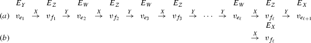
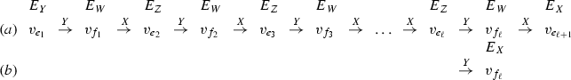
  Let $X'=X\cup \{e_1,\dots ,e_\ell \}\setminus \{f_1,\dots ,f_\ell \}$. Let $Y'=Y\cup \{e_2,\dots ,e_{\ell +1}\}\setminus \{f_1,\dots f_\ell \}$ for case (a), and $Y'=Y\cup \{e_2,\dots ,e_\ell \}\setminus \{f_1,\dots f_{\ell -1}\}$ for case (b). We now have to show that the resulting pair $(X', Y')$ is a pair of spanning trees. Suppose that $X'$ is not a spanning tree. Observe that the X-arcs $(v_{e_1},v_{f_1}),\ldots ,(v_{e_\ell },v_{f_\ell })$ belong to the cycle graph G(X). Thus, by Claim 1, the cycle graph G(X) must contain a subgraph depicted in Fig. 3, where $\{j_1,\dots ,j_\kappa \}\subseteq [\ell ]$. An easy verification shows that all edges $e_i, f_i$, $i\in \{j_1,\dots ,j_\kappa \}$ must have the same costs with respect to $C^*_e$. Indeed, if some costs are different, then there exists an edge exchange which decreases the cost of X. This contradicts our assumption that X is a minimum spanning tree with respect to $C^*_e$. Finally, there must be an arc $(v_{e_{i'}}, v_{f_{i''}})$ in the subgraph such that $i'<i''$. Since $C^*_{e_{i'}}=C^*_{f_{i''}}$, the arc $(v_{e_{i'}}, v_{f_{i''}})$ is present in the admissible graph $G^A$. This leads to a contradiction with our assumption that P is an augmenting path. Now suppose that $Y'$ is not a spanning tree. We consider only the case (a) since the proof of case (b) is just the same. For a convenience, let us number the nodes $v_{e_i}$ on P from $i=0$ to $\ell$, so that $Y'=\{e_1,\dots ,e_{\ell }\}\setminus \{f_1,\dots ,f_{\ell }\}$. The arcs $(v_{e_1}, v_{f_1}), \dots , (v_{e_{\ell }},v_{f_{\ell }})$, which correspond to the Y-arcs $(v_{f_1},v_{e_1}),\dots , (v_{f_{\ell }},v_{e_{\ell }})$ of P, belong to the cycle graph G(Y). Hence, by Claim 1, G(Y) must contain a subgraph depicted in Fig. 3, where $\{i_1,\dots ,i_{\kappa }\}\subseteq [\ell ]$. The rest of the proof is similar to the proof for X. Namely, the edges $e_i$ and $f_i$ for $i\in \{i_1,\dots ,i_{\kappa }\}$ must have the same costs with respect to $c^*_e$. Also, there must exist an arc $(v_{e_{i'}}, v_{f_{{i''}}})$ in the subgraph such that $i'>i''$. In consequence, the arc $(v_{f_{i''}}, v_{e_{i'}})$ belongs to the admissible graph, which contradicts the assumption that P is an augmenting path. An example of the case (a) is shown in Fig. 5. Thus $X'=X\cup \{e_1,e_2,e_3,e_4\}\setminus \{f_1,f_2,f_3,f_4\}$ and $Y'=Y\cup \{e_2,e_3,e_4,e_5\}\setminus \{f_1,f_2,f_3,f_4\}$. An example of the case (b) is shown in Fig. 6. In this example $X'$ is the same as in the previous case and $Y'=Y\cup \{e_2,e_3,e_4\}\setminus \{f_1,f_2,f_3\}$. It is easy to verify that $|E_{Z'}|=|X'\cap Y'|=|E_{Z}|+1$ holds (see also the examples in Figs. 5, 6). The spanning trees $X'$ and $Y'$ are optimal for the costs $C^*_e$ and $c^*_e$, respectively. Furthermore, $E_{X'}\subseteq E_X$ and $E_{Y'}\subseteq E_Y$, so $(X',Y')$ satisfies the sufficient pair optimality conditions (the condition (ii) in Theorem 2 is not violated).

• 3. The augmenting path P is of the form

  

  Let $X'=X\cup \{f_1,\dots ,f_\ell \}\setminus \{e_2,\dots ,e_{\ell +1}\}$ for the case (a) and $X'=X\cup \{f_1,\dots ,f_{\ell -1}\}\setminus \{e_2,\dots e_\ell \}$ for the case (b). Let $Y'=Y\cup \{f_1,\dots ,f_\ell \}\setminus \{e_1,\dots e_\ell \}$. The proof that $X'$ and $Y'$ are spanning trees follows by the same arguments as for the symmetric case described in point 2. An example of the case (a) is shown in Fig. 7. Thus $X'=X\cup \{f_1,f_2,f_3,f_4\}\setminus \{e_2,e_3,e_4,e_5\}$ and $Y'=Y\cup \{f_1,f_2,f_3,f_4\}\setminus \{e_1,e_2,e_3,e_4\}$. An example for the case (b) is shown in Fig. 8. The spanning tree $Y'$ is the same as in the previous case and $X'=X\cup \{f_1,f_2,f_3\}\setminus \{e_2,e_3,e_4\}$. The equality $|E_{Z'|}=|X'\cap Y'|=|E_Z|+1$ holds. Also, the trees $X'$ and $Y'$ are optimal for the costs $C^*_e$ and $c^*_e$, respectively, $E_{X'}\subseteq E_X$, $E_{Y'}\subseteq E_Y$, so $(X',Y')$ satisfies the sufficient pair optimality conditions.$\square$

Fig. 5

A pair (X, Y) and the corresponding admissible graph for the case 2a

Fig. 6

A pair (X, Y) and the corresponding admissible graph for the case 2b

Fig. 7

A pair (X, Y) and the corresponding admissible graph for the case 3a

Fig. 8

A pair (X, Y) and the corresponding admissible graph for the case 3b

We now turn to the case $E_X\cap \{e\in E\,:\, v_e\in V^A\} = \emptyset$. Fix $\delta >0$ (the precise value of $\delta$ will be specified later) and set:

$$\begin{aligned}&C_e(\delta )=C^*_e-\delta ,&c_e(\delta )=c^*_e&v_e \in V^A, \end{aligned}$$

(23a)

$$\begin{aligned}&C_e(\delta )=C^*_e,&c_e(\delta )=c^*_e-\delta&v_e\notin V^A. \end{aligned}$$

(23b)

Lemma 4

There exists a sufficiently small $\delta >0$ such that the costs $C_e(\delta )$ and $c_e(\delta )$ satisfy the path optimality conditions for X and Y, respectively, i.e:

$$\begin{aligned}&\text {for every } e\notin X&C_e(\delta ) \ge C_f(\delta )&\text {for every } f\in P_{X}(e), \end{aligned}$$

(24a)

$$\begin{aligned}&\text {for every } e\notin Y&c_e(\delta ) \ge c_f(\delta )&\text {for every } f\in P_{Y}(e). \end{aligned}$$

(24b)

Proof

If $C^*_e>C^*_f$ (resp. $c^*_e >c^*_f$), $e\notin X, f\in P_{X}(e)$ (resp. $e\notin Y, f\in P_{Y}(e)$), then there is $\delta >0$, such that after setting the new costs (23) the inequality $C_e(\delta )\ge C_f(\delta )$ (resp. $c_e(\delta ) \ge c_f(\delta )$) holds. Hence, one can choose a sufficiently small $\delta >0$ such that after setting the new costs (23), all the strong inequalities are not violated. Therefore, for such a chosen $\delta$ it remains to show that all originally tight inequalities in (22) are preserved for the new costs. Consider a tight inequality of the form:

$$\begin{aligned} C^*_e=C^*_f, \,e\notin X, \quad f\in P_{X}(e). \end{aligned}$$

(25)

On the contrary, suppose that $C_e(\delta )<C_f(\delta )$. This is only possible when $C_e(\delta )=C^*_e-\delta$ and $C_f(\delta )=C^*_f$. Hence and from the construction of the new costs, we have $v_f\notin V^A$ (see (23b)) and $v_e\in V^A$ (see (23a)). By (25), we obtain $(v_e,v_f)\in E^A$. Thus $v_f\in V^A$, a contradiction. Consider a tight inequality of the form:

$$\begin{aligned} c^*_e=c^*_f, \, e\notin Y,\quad f\in P_{Y}(e). \end{aligned}$$

(26)

On the contrary, suppose that $c_e(\delta )<c_f(\delta )$. This is only possible when $c_e(\delta )=c^*_e-\delta$ and $c_f(\delta )=c^*_f$. Thus we deduce that $v_e\notin V^A$ and $v_f\in V^A$ (see (23)). From (26), it follows that $(v_f,v_e)\in E^A$ and so $v_e\in V^A$, a contradiction. $\square$

We are now ready to give the precise value of $\delta$. We do this by increasing the value of $\delta$ until some inequalities, originally not tight in (22), become tight. Namely, let $\delta ^*>0$ be the smallest value of $\delta$ for which an inequality originally not tight becomes tight. Obviously, it occurs when $C^*_e-\delta ^*=C^*_f$ for $e\notin X$, $f\in P_{X}(e)$ or $c^*_f-\delta ^*=c^*_e$ for $f\notin Y$, $e\in P_{Y}(f)$. By (23), $v_e\in V^A$ and $v_f\notin V^A$. Accordingly, if $\delta =\delta ^*$, then at least one arc is added to $G^A$. Observe also that no arc can be removed from $G^A$ - the admissibility of the nodes remains unchanged. It follows from the fact that each tight inequality for $v_e\in V^A$ and $v_f\in V^A$ is still tight. This leads to the following lemma.

Lemma 5

If $E_X\cap \{e\in E\,:\, v_e\in V^A\} = \emptyset$, then (X, Y) satisfies the sufficient pair optimality conditions for each $\theta ' \in [\theta , \theta +\delta ^*]$.

Proof

Set $\theta '=\theta +\delta$, $\delta \in [0, \delta ^*]$. Lemma 4 implies that X is optimal for $C_e(\delta )$ and Y is optimal for $c_e(\delta )$. From (23) and the definition of the costs $C^*_e$ and $c^*_e$, it follows that $C_e(\delta )=C_e-\alpha '_e$ and $c_e(\delta )=c_e-\beta '_e$, where $\alpha _e'=\alpha _e+\delta$ and $\beta '_e=\beta _e$ for each $v_e\in V^A$, $\alpha '_e=\alpha _e$ and $\beta '_e=\beta _e+\delta$ for each $v_e\notin V^A$. Notice that $\alpha '_e+\beta '_e=\alpha _e+\beta _e+\delta =\theta +\delta =\theta '$ for each $e\in E$. By (23), $c_e(\delta )=c_e$ for each $e\in E_Y$ (recall that $e\in E_Y$ implies $v_e\in V^A$), and thus $\beta _e=0$ for each $e\in E_Y$. Since $E_X\cap \{e\in E\,:\, v_e\in V^A\} = \emptyset$, $C_e(\delta )=C^*_e=C_e$ holds for each $e\in E_X$, and so $\alpha _e=0$ for each $e\in E_X$. We thus have shown that there exist $\alpha '_e,\beta '_e \ge 0$ such that $\alpha '_e+\beta '_e= \theta '$ for each $e\in E$ satisfying the conditions (i) and (ii) in Theorem 2, which completes the proof. $\square$

We now describe a polynomial procedure that, for a given pair (X, Y) satisfying the sufficient pair optimality conditions for some $\theta \ge 0$, finds a new pair of spanning trees $(X',Y')$, which also satisfies the sufficient pair optimality conditions with $|E_Z'|=|E_Z|+1$. We start by building the admissible graph $G^A=(V^A,E^A)$ for (X, Y). If this graph contains an augmenting path, then by Lemma 3, we are done. Otherwise, we determine $\delta ^*$ and modify the costs by using (23). Lemma 5 shows that (X, Y) satisfies the sufficient pair optimality conditions for $\theta +\delta ^*$. For $\delta ^*$ some new arcs are added to the admissible graph $G^A$ (all the previous arcs must be still present in $G^A$). Thus $G^A$ is updated and we set $C^*_e:=C_e(\delta ^*)$, $c^*_e:=c_e(\delta ^*)$ for each $e\in E$, and $\theta :=\theta +\delta ^*$. We repeat this until there is an augmenting path in $G^A=(V^A,E^A)$. Note that such a path must appear after at most $m=|E|$ iterations, which follows from the fact that at some step a node $v_e$ such that $e\in E_X$ must appear in $G^A$.

Fig. 9

Sample computations, $X=\{e_2, e_4,e_5,e_6,e_9,e_{10}\}$ and $Y=\{e_2, e_3, e_5, e_8, e_9, e_{11}\}$

Sample computations are shown in Fig. 9. We start with the pair (X, Y), where $X=\{e_2, e_4,e_5,e_6,e_9,e_{10}\}$ and $Y=\{e_2, e_3, e_5, e_8, e_9, e_{11}\}$, which satisfies the sufficient pair optimality conditions for $\theta =0$ (see Fig. 9a). Observe that in this case it is enough to check that X is optimal for the costs $C^*_e=C_e$ and Y is optimal for the costs $c^*_e=c_e$, $e\in E$. For $\theta =0$, the admissible graph does not contain any augmenting path. We thus have to modify the costs $C^*_e$ and $c^*_e$, according to (23). For $\delta ^*=1$, a new inequality becomes tight and one arc is added to the admissible graph (see Fig. 9b). The admissible graph still does not have an augmenting path, so we have to again modify the costs. For $\delta ^*=1$ some new inequalities become tight and three arcs are added to the admissible graph (see Fig. 9c). Now the admissible graph has two augmenting paths (cases 1 and 3a, see the proof of Lemma 3). Choosing one of them, and performing the modification described in the proof of Lemma 3 we get a new pair $(X', Y')$ with $|E_{Z'}|=|E_Z|+1$.

Let us now estimate the running time of the procedure. The admissible graph has at most m nodes and at most mn arcs. It can be built in O(nm) time. The augmenting path in the admissible graph can be found in O(nm) time by applying the breath first search. Also the number of inequalities which must be analyzed to find $\delta ^*$ is O(nm). Since we have to update the cost of each arc of the admissible graph at most m times, until an augmenting path appears, the required time of the procedure is $O(m^2n)$. We thus get the following result.

Theorem 3

The Rec ST problem is solvable in $O(Lm^2n)$ time, where $L=n-1-k$.

3 The recoverable robust spanning tree problem

In this section we are concerned with the Rob Rec ST problem under the interval uncertainty representation, i.e. for the scenario sets $\mathcal {U}^{I}$, $\mathcal {U}^{I}_1(\Gamma )$, and $\mathcal {U}^{I}_2(\Gamma )$. Using the polynomial algorithm for Rec ST, constructed in Sect. 2, we will provide a polynomial algorithm for Rob Rec ST under $\mathcal {U}^{I}$ and some approximation algorithms for a wide class of Rob Rec ST under $\mathcal {U}^{I}_1(\Gamma )$ and $\mathcal {U}^{I}_2(\Gamma )$. The idea will be to solve Rec ST for a suitably chosen second stage costs. Let

$$\begin{aligned} F(X)=\sum _{e\in X} C_e + \max _{S\in \mathcal {U}}\min _{Y\in \Phi ^k_{X}} f(Y,S), \end{aligned}$$

where $f(Y,S)=\sum _{e\in Y} c^S_e$. It is worth pointing out that under scenario sets $\mathcal {U}^{I}$ and $\mathcal {U}^{I}_2(\Gamma )$, the value of F(X), for a given spanning tree X, can be computed in polynomial time (Şeref et al. 2009; Nasrabadi and Orlin 2013). On the other hand, computing F(X) under $\mathcal {U}^{I}_1(\Gamma )$ turns out to be strongly NP-hard (Nasrabadi and Orlin 2013; Frederickson and Solis-Oba 1999). Given scenario $S=(c_e^S)_{e\in E}$, consider the following Rec ST problem:

$$\begin{aligned} \min _{X\in \Phi } \left( \sum _{e\in X} C_e + \min _{Y\in \Phi ^k_X} f(Y,S)\right) . \end{aligned}$$

(27)

Problem (27) is equivalent to the formulation (1) for $S=(c_e)_{e\in E}$ and it is polynomially solvable, according to the result obtained in Sect. 2. As in the previous section, we denote by pair (X, Y) a solution to (27), where $X\in \Phi$ and $Y\in \Phi ^k_X$. Given S, we call (X, Y) an optimal pair under S if (X, Y) is an optimal solution to (27).

The Rob Rec ST problem with scenario set $\mathcal {U}^{I}$ can be rewritten as follows:

$$\begin{aligned} \min _{X\in \Phi } \left( \sum _{e\in X} C_e + \max _{S\in \mathcal {U}^{I}}\min _{Y\in \Phi ^{k}_{X}}\sum _{e\in Y}c^{S}_e \right) = \min _{X\in \Phi } \left( \sum _{e\in X} C_e + \min _{Y\in \Phi ^{k}_{X}} \sum _{e\in E}(c_e+d_e) \right) . \end{aligned}$$

(28)

Thus (28) is (27) for $S=(c_e+d_e)_{e\in E}\in \mathcal {U}^{I}$. Hence and from Theorem 3 we immediately get the following theorem:

Theorem 4

For scenario set $\mathcal {U}^I$, the Rob Rec ST problem is solvable in $O((n-1-k)m^2n)$ time.

We now address Rob Rec ST under $\mathcal {U}^{I}_1(\Gamma )$ and $\mathcal {U}^{I}_2(\Gamma )$. Suppose that $c_e\ge \alpha (c_e+d_e)$ for each $e\in E$, where $\alpha \in (0,1]$ is a given constant. This inequality means that for each edge $e\in E$ the nominal cost $c_e$ is positive and $c_e+d_e$ is at most $1/\alpha$ greater than $c_e$. It is reasonable to assume that this condition will be true in many practical applications for not very large value of $1/\alpha$.

Lemma 6

Suppose that $c_e\ge \alpha (c_e+d_e)$ for each $e\in E$, where $\alpha \in (0,1]$, and let $(\hat{X}, \hat{Y})$ be an optimal pair under $\underline{S}=(c_e)_{e\in E}$. Then for the scenario sets $\mathcal {U}^{I}_1(\Gamma )$ and $\mathcal {U}^{I}_2(\Gamma )$ the inequality $F(\hat{X})\le \frac{1}{\alpha } F(X)$ holds for any $X\in \Phi$.

Proof

We give the proof only for the scenario set $\mathcal {U}^{I}_1(\Gamma )$. The proof for $\mathcal {U}^{I}_2(\Gamma )$ is the same. Let $X\in \Phi$. The following inequality is satisfied:

$$\begin{aligned} F(X)=\sum _{e\in X} C_e+\max _{S\in \mathcal {U}_1^I(\Gamma )}\min _{Y\in \Phi ^k_X}f(Y,S)=\sum _{e\in X} C_e+f(Y^*,S^*)\ge \sum _{e\in X} C_e+ f(Y^*,\underline{S}). \end{aligned}$$

Clearly, $(X,Y^*)$ is a feasible pair to (27) under $\underline{S}$. From the definition of $(\hat{X},\hat{Y})$ we get

$$\begin{aligned} F(X)\ge \sum _{e\in \hat{X}} C_e+ f(\hat{Y},\underline{S})= & {} \sum _{e\in \hat{X}} C_e + \sum _{e\in \hat{Y}} c_e \ge \sum _{e\in \hat{X}} C_e + \sum _{e\in \hat{Y}} \alpha (c_e+d_e)\nonumber \\= & {} \sum _{e\in \hat{X}} C_e+ \alpha f(\hat{Y},\overline{S}), \end{aligned}$$

(29)

where $\overline{S}=(c_e+d_e)_{e\in E}$. Hence

$$\begin{aligned} F(X)&\ge \sum _{e\in \hat{X}} C_e +\alpha \max _{S \in \mathcal {U}_1^I(\Gamma )}f(\hat{Y},S) \ge \sum _{e\in \hat{X}} C_e +\alpha \max _{S \in \mathcal {U}_1^I(\Gamma )}\min _{Y\in \Phi ^k_{\hat{X}}}f(Y, S) \\&\ge \alpha \left( \sum _{e\in \hat{X}} C_e + \max _{S \in \mathcal {U}_1^I(\Gamma )}\min _{Y\in \Phi ^k_{\hat{X}}}f(Y, S)\right) =\alpha F(\hat{X}) \end{aligned}$$

and the lemma follows. $\square$

The condition $c_e\ge \alpha (c_e+d_e)$, $e\in E$, in Lemma 6, can be weakened and, in consequence, the set of instances to which the approximation ratio of the algorithm applies can be extended. Indeed, from inequality (29) it follows that the bounds of the uncertainty intervals are only required to meet the condition $\sum _{e\in \hat{Y}} c_e \ge \alpha \sum _{e\in \hat{Y}}(c_e+d_e)$. This condition can be verified efficiently, since $\hat{Y}$ can be computed in polynomial time.

We now focus on Rob Rec ST for $\mathcal {U}^{I}_2(\Gamma )$. Define $D=\sum _{e\in E} d_e$ and suppose that $D>0$ (if $D=0$, then the problem is equivalent to Rec ST for the second stage costs $c_e$, $e\in E$). Consider scenario $S'$ under which $c_e^{S'}=\min \{c_e+d_e, c_e+\Gamma \frac{d_e}{D}\}$ for each $e\in E$. Obviously, $S'\in \mathcal {U}^{I}_2(\Gamma )$, since $\sum _{e\in E} \delta _e \le \sum _{e\in E} \Gamma \frac{d_e}{D}\le \Gamma$. The following theorem provides another approximation result for Rob Rec ST with scenario set $\mathcal {U}^{I}_2(\Gamma )$:

Lemma 7

Let $(\hat{X}, \hat{Y})$ be an optimal pair under $S'$. Then the following implications are true for scenario set $\mathcal {U}^{I}_2(\Gamma )$:

• (i) If $\Gamma \ge \beta D$, $\beta \in (0,1]$, then $F(\hat{X})\le \frac{1}{\beta }F(X)$ for any $X\in \Phi$.

• (ii) If $\Gamma \le \gamma F(\hat{X})$, $\gamma \in [0,1)$ then $F(\hat{X})\le \frac{1}{1-\gamma }F(X)$ for any $X\in \Phi$.

Proof

Let $X\in \Phi$. Since $S'\in \mathcal {U}^{I}_2(\Gamma )$, we get

$$\begin{aligned} F(X)= \sum _{e\in X} C_e+\max _{S\in \mathcal {U}_2^I(\Gamma )}\min _{Y\in \Phi ^k_X}f(Y,S)\ge \sum _{e\in X} C_e+\min _{Y\in \Phi ^k_{X}}f(Y,S'). \end{aligned}$$

(30)

We first prove implication (i). By (30) and the definition of $(\hat{X},\hat{Y})$, we obtain

$$\begin{aligned} F(X)&\ge \sum _{e\in \hat{X}} C_e+f(\hat{Y},S') =\sum _{e\in \hat{X}} C_e+ \sum _{e\in \hat{Y}} \min \left\{ c_e+d_e, c_e+\Gamma \frac{d_e}{D}\right\} \\&\ge \sum _{e\in \hat{X}} C_e+ \sum _{e\in \hat{Y}} \min \left\{ c_e+d_e, c_e+\beta d_e\right\} = \sum _{e\in \hat{X}} C_e\\&\quad + \sum _{e\in \hat{Y}} (c_e+\beta d_e)\ge \sum _{e\in \hat{X}} C_e+ \beta f(\hat{Y},\overline{S}), \end{aligned}$$

where $\overline{S}=(c_e+d_e)_{e\in E}$. The rest of the proof is the same as in the proof of Lemma 6. We now prove implication (ii). By (30) and the definition of $(\hat{X},\hat{Y})$, we have

$$\begin{aligned} F(X)&\ge \sum _{e\in \hat{X}} C_e+f(\hat{Y},S') \ge \sum _{e\in \hat{X}} C_e+f(\hat{Y},\underline{S})\ge \sum _{e\in \hat{X}} C_e+ \max _{S\in \mathcal {U}_2^I(\Gamma )}f(\hat{Y},S)-\Gamma \\&\ge \sum _{e\in \hat{X}} C_e+ \max _{S\in \mathcal {U}_2^I(\Gamma )} \min _{Y\in \Phi ^k_{\hat{X}}}f(Y,S)-\Gamma =F(\hat{X})-\Gamma . \end{aligned}$$

If $\Gamma \le \gamma F(\hat{X})$. Then $F(X)\ge F(\hat{X})-\gamma F(\hat{X})=(1-\gamma )F(\hat{X})$ and $F(\hat{X})\le \frac{1}{1-\gamma } F(X).$ $\square$

Note that the value of $F(\hat{X})$ under $\mathcal {U}^{I}_2(\Gamma )$ can be computed in polynomial time (Nasrabadi and Orlin 2013). In consequence, the constants $\beta$ and $\gamma$ can be efficiently determined for every particular instance of the problem. Clearly, we can assume that $d_e\le \Gamma$ for each $e\in E$, which implies $D\le m\Gamma$, where $m=|E|$. Hence, we can assume that $\Gamma \ge \frac{1}{m} D$ for every instance of the problem. We thus get from Lemma 7 (implication (i)) that $F(\hat{X})\le m F(X)$ for any $X\in \Phi$ and the problem is approximable within m. If $\alpha$, $\beta$ and $\gamma$ are the constants from Lemmas 6 and 7, then the following theorem summarizes the approximation results:

Theorem 5

Rob Rec ST is approximable within $\frac{1}{\alpha }$ under scenario set $\mathcal {U}^{I}_1(\Gamma )$ and it is approximable within $\min \{\frac{1}{\beta },\frac{1}{\alpha },\frac{1}{1-\gamma }\}$ under scenario set $\mathcal {U}^{I}_2(\Gamma )$.

Observe that Lemmas 6 and 7 hold of any sets $\Phi$ and $\Phi ^k_X$ (the particular structure of these sets is not exploited). Hence the approximation algorithms can be applied to any problem for which the recoverable version (27) is polynomially solvable.

4 Conclusions

In this paper we have studied the recoverable robust spanning tree problem (Rob Rec ST) under various interval uncertainty representations. The main result is the polynomial time combinatorial algorithm for the recoverable spanning tree. We have applied this algorithm for solving Rob Rec ST under the traditional uncertainty representation (see, e.g., Kouvelis and Yu 1997) in polynomial time. Moreover, we have used the algorithm for providing several approximation results for Rec ST with the scenario set introduced by Bertsimas and Sim (2003) and the scenario set with a budged constraint (see, e.g,. Nasrabadi and Orlin 2013). There is a number of open questions concerning the considered problem. Perhaps, the most interesting one is to resolve the complexity of the robust problem under the interval uncertainty representation with budget constraint. It is possible that this problem may be solved in polynomial time by some extension of the algorithm constructed in this paper. One can also try to extend the algorithm for the more general recoverable matroid base problem, which has also been shown to be polynomially solvable in Hradovich et al. (2016).

References

Ahuja RK, Magnanti TL, Orlin JB (1993) Network flows: theory, algorithms, and applications. Prentice Hall, Englewood Cliffs
Aissi H, Bazgan C, Vanderpooten D (2007) Approximation of min-max and min-max regret versions of some combinatorial optimization problems. Eur J Oper Res 179:281–290
Bertsimas D, Sim M (2003) Robust discrete optimization and network flows. Math Program 98:49–71
Büsing C (2011) Recoverable robustness in combinatorial optimization. PhD thesis, Technical University of Berlin, Berlin
Büsing C (2012) Recoverable robust shortest path problems. Networks 59:181–189
Büsing C, Koster AMCA, Kutschka M (2011) Recoverable robust knapsacks: the discrete scenario case. Optim Lett 5:379–392
Chassein A, Goerigk M (2015) On the recoverable robust traveling salesman problem. Optim Lett. doi:10.1007/s11590-015-0949-5
Frederickson NG, Solis-Oba R (1999) Increasing the weight of minimum spanning trees. J Algorithm 33:244–266
Hradovich M, Kasperski A, Zieliński P (2016) The recoverable robust spanning tree problem with interval costs is polynomially solvable. Optim Lett. doi:10.1007/s11590-016-1057-x
Kasperski A, Kurpisz A, Zieliński P (2014) Recoverable robust combinatorial optimization problems. Oper Res Proc 2012:147–153
Kasperski A, Zieliński P (2011) On the approximability of robust spanning problems. Theor Comput Sci 412:365–374
Kouvelis P, Yu G (1997) Robust discrete optimization and its applications. Kluwer Academic, Norwell
Lau LC, Ravi R, Singh M (2011) Iterative methods in combinatorial optimization. Cambridge University Press, Cambridge
Liebchen C, Lübbecke ME, Möhring RH, Stiller S (2009) The concept of recoverable robustness, linear programming recovery, and railway applications. In: Robust and online large-scale optimization. Lecture notes in computer science, vol 5868. Springer, New York, pp 1–27
Lin K, Chern MS (1993) The most vital edges in the minimum spanning tree problem. Inf Process Lett 45:25–31
Nasrabadi E, Orlin JB (2013) Robust optimization with incremental recourse. CoRR, abs/1312.4075
Papadimitriou CH, Steiglitz K (1998) Combinatorial optimization: algorithms and complexity. Dover, Mineola
Şeref O, Ahuja RK, Orlin JB (2009) Incremental network optimization: theory and algorithms. Oper Res 57:586–594
Acknowledgments
The second and the third authors were supported by the National Center for Science (Narodowe Centrum Nauki), Grant 2013/09/B/ST6/01525.
Author information
Authors and Affiliations
Corresponding author
Rights and permissions
Open Access This article is distributed under the terms of the Creative Commons Attribution 4.0 International License (http://creativecommons.org/licenses/by/4.0/), which permits unrestricted use, distribution, and reproduction in any medium, provided you give appropriate credit to the original author(s) and the source, provide a link to the Creative Commons license, and indicate if changes were made.
About this article
Cite this article
Hradovich, M., Kasperski, A. & Zieliński, P. Recoverable robust spanning tree problem under interval uncertainty representations. J Comb Optim 34, 554–573 (2017). https://doi.org/10.1007/s10878-016-0089-6
Published:
Issue Date:
DOI: https://doi.org/10.1007/s10878-016-0089-6