
Abstract
This paper studies Gaussian-based filters within the pseudo-marginal Metropolis Hastings (PM-MH) algorithm for posterior inference on parameters in nonlinear DSGE models. We implement two Gaussian-based filters to evaluate the likelihood of a DSGE model solved to second and third order and embed them into the PM-MH: Central Difference Kalman filter (CDKF) and Gaussian mixture filter (GMF). The GMF is adaptively refined by splitting a mixture component into new mixture components based on Binomial Gaussian mixture. The overall results indicate that the estimation accuracy of the CDKF and the GMF is comparable to that of the particle filter (PF), except that the CDKF generates biased estimates in the extremely nonlinear case. The proposed GMF generates the most accurate estimates among them. We argue that the GMF with PM-MH can converge to the true and invariant distribution when the likelihood constructed by infinite Gaussian mixtures weakly converges to the true likelihood. In addition, we show that the Gaussian-based filters are more efficient than the PF in terms of effective computing time. Finally, we apply the method to real data.


Notes
We tested other Sigma-Point Kalman filters (UKF and CKF) for the likelihood evaluation and posterior inference on parameters in the application of our neoclassical growth model solved up to second and third order. However, the UKF, the CDKF, and the CKF show similar performance. The estimation results are available upon request.
We can apply the GMF to models with non-Gaussian structural shocks and measurement errors by estimating the Gaussian mixture densities of the structural shocks and the measurement errors. The Gaussian mixture densities can be estimated using an Expectation Maximization (EM) algorithm (McLachlan and Peel 2004.
Runnalls (2007) proposes the following KL-based discrimination measure:
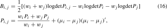
where \(\mu _i\) is the (predictive or filtered) mean for component i, \(w_i\) is the weight for mixture component i, and \(P_i\) is the (predictive or filtered) covariance matrix for component i.
We greatly thank Martin M. Andreasen for making publicly available his codes for the optimized central difference particle filter.
The higher-order approximations create explosive sample paths because the higher-order terms generate unstable steady states. To deal with this problem, it is recommended to apply pruning scheme that omits terms of higher-order effects (Kim et al. 2008). However, the simulated sample paths without pruning are stable and are not much different from those obtained with pruning in our case. Moreover, the estimation results without pruning are consistent with those with pruning so that we will report the results obtained without pruning. The estimation results obtained with pruning are available upon request.
The CDKF might not satisfy these sufficient conditions, depending on how nonlinear the model is. According to the Monte Carlo exercises in Sect. 5, the CDKF seems to satisfy the conditions in the benchmark and nearly linear cases (except for a few cases in the benchmark case), but does not satisfy the conditions when the model is highly nonlinear.
Mengersen and Tweedie (1996) and Roberts and Tweedie (1996) verify that a random-walk-based Metropolis is geometrically ergodic when the target invariant distribution has exponentially decreasing tails (in one dimension) and behaves sufficiently smoothly in the tails (in higher dimension). Jarner and Hansen (2000) shows more general conditions for geometric ergodicity. Although a random-walk-based MH sampler might fail to satisfy these conditions, it can be polynomially ergodic of all orders (Fort and Moulines 2000).
We calculate the scores \(\hat{s}^k_t(\theta )\) and the Hessians \(\hat{h}^k_t(\theta )\) by numerically differentiating the conditional likelihoods \(\hat{l}^k_t(\theta )\)
The effective sample size is used to assess the convergence of sums of MCMC samples in a heuristic way.
The coefficient of variation is calculated as
$$\begin{aligned} CV=\frac{var(h)}{E[h]^2}=exp\Bigg (\frac{\sigma _{\sigma _z}^2}{1-\rho _{\sigma _z}^2}\Bigg )-1. \end{aligned}$$When setting \(\rho _{\sigma _z}=0.9\) and \(\sigma _{\sigma _z}=0.135\), the CV is 0.1. In that case, the estimation result for \(\rho _{\sigma _z}\) becomes poorer, though the result for \(\sigma _{\sigma _z}\) is not bad. The estimation results are given in “Appendix E”.

References
Achieser, N. I. (2013). Theory of approximation. North Chelmsford: Courier Corporation.
Ali-Löytty, S. (2008). On the convergence of the Gaussian mixture filter. Tampere: Tampere University of Technology.
Alspach, D. L., & Sorenson, H. W. (1971). Recursive Bayesian estimation using Gaussian sums. Automatica, 7(4), 465–479. https://doi.org/10.1016/0005-1098(71)90097-5.
Alspach, D. L., & Sorenson, H. W. (1972). Nonlinear Bayesian estimation using Gaussian sum approximations. IEEE Transactions on Automatic Control, 17(4), 439–448. https://doi.org/10.1109/TAC.1972.1100034.
Amisano, G., & Tristani, O. (2010). Euro area inflation persistence in an estimated nonlinear DSGE model. Journal of Economic Dynamics and Control, 34(10), 1837–1858. https://doi.org/10.1016/j.jedc.2010.05.001.
An, S., & Schorfheide, F. (2007). Bayesian analysis of DSGE models. Econometric Reviews, 26(2–4), 113–172. https://doi.org/10.1080/07474930701220071.
Andreasen, M. M. (2011). Non-linear DSGE models and the optimized central difference particle filter. Journal of Economic Dynamics and Control, 35(10), 1671–1695. https://doi.org/10.1016/j.jedc.2011.04.007.
Andreasen, M. M. (2012). On the effects of rare disasters and uncertainty shocks for risk premia in non-linear DSGE models. Review of Economic Dynamics, 15(3), 295–316. https://doi.org/10.1016/j.red.2011.08.001.
Andreasen, M. M. (2013). Non-linear DSGE models and the central difference Kalman filter. Journal of Applied Econometrics, 28(6), 929–955. https://doi.org/10.1002/jae.2282.
Andrieu, C., Doucet, A., & Holenstein, R. (2010). Particle Markov chain Monte Carlo methods. Journal of the Royal Statistical Society: Series B (Statistical Methodology), 72(3), 269–342. https://doi.org/10.1111/j.1467-9868.2009.00736.x.
Andrieu, C., & Roberts, G. O. (2009). The pseudo-marginal approach for efficient Monte Carlo computations. The Annals of Statistics, 37, 697–725.
Arasaratnam, I., & Haykin, S. (2009). Cubature Kalman filters. IEEE Transactions on Automatic Control, 54(6), 1254–1269. https://doi.org/10.1109/TAC.2009.2019800.
Basu, S., & Bundick, B. (2017). Uncertainty shocks in a model of effective demand. Econometrica, 85(3), 937–958. https://doi.org/10.3982/ECTA13960.
Binning, A. & Maih, J. (2015). Sigma point filters for dynamic nonlinear regime switching models. Working paper, Norges Bank. https://ideas.repec.org/p/bno/worpap/2015_10.html.
Bollerslev, T., & Wooldridge, J. M. (1992). Quasi-maximum likelihood estimation and inference in dynamic models with time-varying covariances. Econometric Reviews, 11(2), 143–172. https://doi.org/10.1080/07474939208800229.
Bonciani, D., & van Roye, B. (2016). Uncertainty shocks, banking frictions and economic activity. Journal of Economic Dynamics and Control, 73, 200–219. https://doi.org/10.1016/j.jedc.2016.09.008.
Born, B., & Pfeifer, J. (2014). Policy risk and the business cycle. Journal of Monetary Economics, 68, 68–85. https://doi.org/10.1016/j.jmoneco.2014.07.012.
Brock, W. A., & Mirman, L. J. (1972). Optimal economic growth and uncertainty: The discounted case. Journal of Economic Theory, 4(3), 479–513. https://doi.org/10.1016/0022-0531(72)90135-4.
Canova, F., & Sala, L. (2009). Back to square one: Identification issues in DSGE models. Journal of Monetary Economics, 56(4), 431–449. https://doi.org/10.1016/j.jmoneco.2009.03.014.
Chopin, N. (2004). Central limit theorem for sequential Monte Carlo methods and its application to Bayesian inference. The Annals of Statistics, 32, 2385–2411. https://doi.org/10.1214/009053604000000698.
DeJong, D. N., Liesenfeld, R., Moura, G. V., Richard, J.-F., & Dharmarajan, H. (2012). Efficient likelihood evaluation of state-space representations. Review of Economic Studies, 80(2), 538–567. https://doi.org/10.1093/restud/rds040.
Fernández-Villaverde, J. (2010). The econometrics of DSGE models. SERIEs, 1(1–2), 3–49. https://doi.org/10.1007/s13209-009-0014-7.
Fernández-Villaverde, J., Guerrón-Quintana, P., Kuester, K., & Rubio-Ramírez, J. (2015). Fiscal volatility shocks and economic activity. American Economic Review, 105(11), 3352–3384. https://doi.org/10.1257/aer.20121236.
Fernández-Villaverde, J., Guerrón-Quintana, P., Rubio-Ramírez, J. F., & Uribe, M. (2011). Risk matters: The real effects of volatility shocks. American Economic Review, 101(6), 2530–2561. https://doi.org/10.1257/aer.101.6.2530.
Fernández-Villaverde, J., & Levintal, O. (2016). Solution methods for models with rare disasters. Technical report, National Bureau of Economic Research.
Fernández-Villaverde, J., & Rubio-Ramírez, J. F. (2005). Estimating dynamic equilibrium economies: Linear versus nonlinear likelihood. Journal of Applied Econometrics, 20(7), 891–910. https://doi.org/10.1002/jae.814.
Fernández-Villaverde, J., & Rubio-Ramírez, J. F. (2007). Estimating macroeconomic models: A likelihood approach. Review of Economic Studies, 74(4), 1059–1087. https://doi.org/10.1111/j.1467-937X.2007.00437.x.
Fort, G., & Moulines, E. (2000). V-subgeometric ergodicity for a Hastings–Metropolis algorithm. Statistics and Probability Letters, 49(4), 401–410. https://doi.org/10.1016/S0167-7152(00)00074-2.
Geweke, J. (1999). Using simulation methods for Bayesian econometric models: Inference, development, and communication. Econometric Reviews, 18(1), 1–73. https://doi.org/10.1080/07474939908800428.
Geweke, J. (2005). Contemporary Bayesian econometrics and statistics (Vol. 537). New York: Wiley.
Hall, J., Pitt, M. K., & Kohn, R. (2014). Bayesian inference for nonlinear structural time series models. Journal of Econometrics, 179(2), 99–111. https://doi.org/10.1016/j.jeconom.2013.10.016.
Hall, P., & Heyde, C. C. (2014). Martingale limit theory and its application. Cambridge: Academic Press.
Hansen, G. D. (1985). Indivisible labor and the business cycle. Journal of Monetary Economics, 16(3), 309–327. https://doi.org/10.1016/0304-3932(85)90039-X.
Herbst, E. (2015). Using the “Chandrasekhar Recursions” for likelihood evaluation of DSGE models. Computational Economics, 45(4), 693–705. https://doi.org/10.1007/s10614-014-9430-2.
Herbst, E., & Schorfheide, F. (2017). Tempered particle filtering. Journal of Econometrics, 210, 26–44.
Jacquier, E., Polson, N. G., & Rossi, P. E. (2002). Bayesian analysis of stochastic volatility models. Journal of Business and Economic Statistics, 20(1), 69–87. https://doi.org/10.1198/073500102753410408.
Jarner, S. F., & Hansen, E. (2000). Geometric ergodicity of Metropolis algorithms. Stochastic Processes and Their Applications, 85(2), 341–361. https://doi.org/10.1016/S0304-4149(99)00082-4.
Jazwinski, A. H. (1970). Stochastic processes and filtering theory. Cambridge: Academic Press.
Julier, S. J., & Uhlmann, J. K. (1997). A new extension of the Kalman filter to nonlinear systems. In International symposium of aerospace/defense sensing, simulation and controls (Vol. 3, No. 26, pp. 182–193). https://doi.org/10.1117/12.280797.
Justiniano, A., & Primiceri, G. E. (2008). The time-varying volatility of macroeconomic fluctuations. American Economic Review, 98(3), 604–41. https://doi.org/10.1257/aer.98.3.604.
Justiniano, A., Primiceri, G. E., & Tambalotti, A. (2010). Investment shocks and business cycles. Journal of Monetary Economics, 57(2), 132–145. https://doi.org/10.1016/j.jmoneco.2009.12.008.
Kim, J., & Kim, S. H. (2003). Spurious welfare reversals in international business cycle models. Journal of International Economics, 60(2), 471–500. https://doi.org/10.1016/S0022-1996(02)00047-8.
Kim, J., Kim, S., Schaumburg, E., & Sims, C. A. (2008). Calculating and using second-order accurate solutions of discrete time dynamic equilibrium models. Journal of Economic Dynamics and Control, 32(11), 3397–3414. https://doi.org/10.1016/j.jedc.2008.02.003.
Kim, S., Shephard, N., & Chib, S. (1998). Stochastic volatility: Likelihood inference and comparison with ARCH models. The Review of Economic Studies, 65(3), 361–393. https://doi.org/10.1111/1467-937X.00050.
King, R. G., Plosser, C. I., & Rebelo, S. T. (1988a). Production, growth and business cycles: I. The basic neoclassical model. Journal of Monetary Economics, 21(2–3), 195–232. https://doi.org/10.1016/0304-3932(88)90030-X.
King, R. G., Plosser, C. I., & Rebelo, S. T. (1988b). Production, growth and business cycles: II. New directions. Journal of Monetary Economics, 21(2–3), 309–341. https://doi.org/10.1016/0304-3932(88)90034-7.
Leduc, S., & Liu, Z. (2016). Uncertainty shocks are aggregate demand shocks. Journal of Monetary Economics, 82, 20–35. https://doi.org/10.1016/j.jmoneco.2016.07.002.
Lo, J. (1972). Finite-dimensional sensor orbits and optimal nonlinear filtering. IEEE Transactions on Information Theory, 18(5), 583–588. https://doi.org/10.1109/TIT.1972.1054885.
McLachlan, G., & Peel, D. (2004). Finite mixture models. New York: Wiley.
Mengersen, K. L., & Tweedie, R. L. (1996). Rates of convergence of the Hastings and Metropolis algorithms. The Annals of Statistics, 24(1), 101–121. https://doi.org/10.1214/aos/1033066201.
Meyn, S. P., & Tweedie, R. L. (2012). Markov chains and stochastic stability. Berlin: Springer.
Müller, U. K. (2013). Risk of Bayesian inference in misspecified models, and the sandwich covariance matrix. Econometrica, 81(5), 1805–1849. https://doi.org/10.3982/ECTA9097.
Mumtaz, H., & Theodoridis, K. (2015). The international transmission of volatility shocks: An empirical analysis. Journal of the European Economic Association, 13(3), 512–533. https://doi.org/10.1111/jeea.12120.
Mumtaz, H., & Zanetti, F. (2013). The impact of the volatility of monetary policy shocks. Journal of Money, Credit and Banking, 45(4), 535–558. https://doi.org/10.1111/jmcb.12015.
Niemi, J., & West, M. (2010). Adaptive mixture modeling Metropolis methods for Bayesian analysis of nonlinear state-space models. Journal of Computational and Graphical Statistics, 19(2), 260–280. https://doi.org/10.1198/jcgs.2010.08117.
NøRgaard, M., Poulsen, N. K., & Ravn, O. (2000). New developments in state estimation for nonlinear systems. Automatica, 36(11), 1627–1638. https://doi.org/10.1016/S0005-1098(00)00089-3.
Omori, Y., Chib, S., Shephard, N., & Nakajima, J. (2007). Stochastic volatility with leverage: Fast and efficient likelihood inference. Journal of Econometrics, 140(2), 425–449. https://doi.org/10.1016/j.jeconom.2006.07.008.
Pitt, M. K., dos Santos Silva, R., Giordani, P., & Kohn, R. (2012). On some properties of Markov chain Monte Carlo simulation methods based on the particle filter. Journal of Econometrics, 171(2), 134–151. https://doi.org/10.1016/j.jeconom.2012.06.004.
Primiceri, G. E. (2005). Time varying structural vector autoregressions and monetary policy. The Review of Economic Studies, 72(3), 821–852. https://doi.org/10.1111/j.1467-937X.2005.00353.x.
Raitoharju, M., & Ali-Loytty, S. (2012). An adaptive derivative free method for Bayesian posterior approximation. IEEE Signal Processing Letters, 19(2), 87–90. https://doi.org/10.1109/LSP.2011.2179800.
Raitoharju, M., Ali-Löytty, S., & Piché, R. (2015). Binomial Gaussian mixture filter. EURASIP Journal on Advances in Signal Processing, 2015(1), 36. https://doi.org/10.1186/s13634-015-0221-2.
Roberts, G. O., & Rosenthal, J. S. (1998). Markov-chain Monte Carlo: Some practical implications of theoretical results. Canadian Journal of Statistics, 26(1), 5–20. https://doi.org/10.2307/3315667.
Roberts, G. O., & Smith, A. F. (1994). Simple conditions for the convergence of the Gibbs sampler and Metropolis–Hastings algorithms. Stochastic Processes and Their Applications, 49(2), 207–216. https://doi.org/10.1016/0304-4149(94)90134-1.
Roberts, G. O., & Tweedie, R. L. (1996). Geometric convergence and central limit theorems for multidimensional Hastings and Metropolis algorithms. Biometrika, 83(1), 95–110. https://doi.org/10.1093/biomet/83.1.95.
Rogerson, R. (1988). Indivisible labor, lotteries and equilibrium. Journal of Monetary Economics, 21(1), 3–16. https://doi.org/10.1016/0304-3932(88)90042-6.
Rudebusch, G. D., & Swanson, E. T. (2012). The bond premium in a DSGE model with long-run real and nominal. American Economic Journal: Macroeconomics, 4(1), 105–143.
Runnalls, A. R. (2007). Kullback–Leibler approach to Gaussian mixture reduction. IEEE Transactions on Aerospace and Electronic Systems, 43(3), 989–999. https://doi.org/10.1109/TAES.2007.4383588.
Schmitt-Grohé, S., & Uribe, M. (2004). Solving dynamic general equilibrium models using a second-order approximation to the policy function. Journal of Economic Dynamics and Control, 28(4), 755–775. https://doi.org/10.1016/S0165-1889(03)00043-5.
Sims, E. R. (2011). Permanent and transitory technology shocks and the behavior of hours: A challenge for DSGE models. Working paper, University of Notre Dame.
Strid, I., & Walentin, K. (2009). Block Kalman filtering for large-scale DSGE models. Computational Economics, 33(3), 277–304. https://doi.org/10.1007/s10614-008-9160-4.
Tierney, L. (1994). Markov chains for exploring posterior distributions. The Annals of Statistics, 22(4), 1701–1728.
Van Der Merwe, R., & Wan, E. A. (2003). Gaussian mixture sigma-point particle filters for sequential probabilistic inference in dynamic state-space models. In 2003 IEEE international conference on acoustics, speech, and signal processing, 2003. Proceedings (ICASSP’03) (Vol. 6, VI–701). https://doi.org/10.1109/ICASSP.2003.1201778.
Vats, D., Flegal, J. M., & Jones, G. L. (2017). Multivariate output analysis for Markov chain Monte Carlo. Working paper. arXiv:1512.07713.
Vihola, M. (2012). Robust adaptive Metropolis algorithm with coerced acceptance rate. Statistics and Computing, 22(5), 997–1008. https://doi.org/10.1007/s11222-011-9269-5.
White, H. (1982). Maximum likelihood estimation of misspecified models. Econometrica, 50(1), 1–25. https://doi.org/10.2307/1912526.
Author information
Authors and Affiliations
Corresponding author
Additional information
Publisher's Note
Springer Nature remains neutral with regard to jurisdictional claims in published maps and institutional affiliations.
I am deeply indebted to my advisor, Christopher Otrok, for his guidance at all stages of this research project. I am also grateful to Scott Holan, Shawn Ni, Isaac Miller, and Kyungsik Nam for useful feedback. I thank participants at CEF (2017).
Appendices
Central Difference Kalman Filter
We define the following matrices which make it possible to match the first-order terms,
and the second-order terms in a Taylor series expansion of our nonlinear state space Eqs. (2) and (3) (Andreasen 2013),
where \(g_l(\cdot )\) and \(h_l(\cdot )\) are lth equation of \(g(\cdot )\) and \(h(\cdot )\), respectively. The sigma-points are used to evaluate the mean and covariance matrix of prediction density:
The above prediction step gives the Gaussian-based prediction density \(p(x_t|y_{1:t-1};\theta )\approx N(\hat{x}_{t|t-1},P^x_{t|t-1})\) where \(P^x_{t|t-1}=S^x_{t|t-1}{S^x_{t|t-1}}'\). The predictions are then updated using the standard Kalman filter updating rule:
where \(S_v\) is the upper triangular Cholesky factorization of R\(_v\). The updating step gives \(p(x_t|y_{1:t};\theta )\approx N(\hat{x}_{t|t},P^x_{t|t})\) where \(P^x_{t|t}=S^x_{t|t}{S^x_{t|t}}'\). Finally we can get the following conditional marginal likelihood,
where \(P^y_{t|t-1}=S^y_{t|t-1}{S^y_{t|t-1}}'\).
Binomial Gaussian Mixture
Following Raitoharju et al. (2015), the Binomial Gaussian mixture splits a normal distributed mixture component of the prediction and filtering density into smaller ones using weights and transformed locations from the binomial distribution. The probability density function of the standardized binomial distribution with the smallest error is expressed using Dirac delta notation as
where m denotes the number of the composite components. According to Berry–Essen theorem, the \(P_{B,m}\) converges to the standard normal distribution as m increases. Based on this well-known property, the Binomial Gaussian mixture is constructed using a mixture of standard normal distributions of which component means, covariance matrices, and weights are chosen based on a scaled binomial distribution. A proper affine transformation allows the mixture product to preserve the mean and covariance of the original Gaussian distribution.
A Binomial Gaussian mixture with \(m_{total}=\prod ^{n}_{i=1}m_i\) components has the following representation
where
\(m_i\) is the number of components in ith binomial distribution, \(\sigma _i\) is the variance in ith binomial distribution, T is the operator for the affine transformation, and C is the Cartesian product
Notation \(C_{l,i}\) is the ith component of the lth combination. If \(m_k=1\), the term \(\frac{2C_{l,k}-m_k-1}{\sqrt{m_k -1}}\) is set to 0.
Raitoharju et al. (2015) use the notation to define a random variable \({\varvec{x}}_{{\varvec{BinoGM}}}\) distributed according to the above Binomial Gaussian mixture.
They show that
The Eq. (79) implies that the Binomial Gaussian mixture converges to the original Gaussian distribution in the limit. In splitting a mixture component, the parameters are chosen such that the mean and covariance are preserved. The mean is preserved by choosing \(\mu \) in (73) to be the mean of the mixture component. If the component covariance matrix is \(P_0\) and it is split into smaller components that have covariance P, matrices T and \(\Sigma \) have to be chosen so that
The parameters for the Binomial Gaussian mixture are chosen such that it is a good approximation of the original mixture component, the nonlinearity is below a predetermined threshold \(\eta _{limit}\), two equally weighted components that are next to each other produce a unimodal pdf, and the number of components is minimized (see Appendix in Raitoharju et al. 2015). Under these conditions, the matrix T is chosen as
where \(L(P_0)\) is the square root matrix of \(P_0\), \(\sigma _i^2=m_i-1\), \(\frac{\lambda _i^2}{m_i^2}=\frac{\lambda _j^2}{m_j^2}\) with the conditions that \(m_i\ge 1\), \(\frac{1}{R}\sum ^n_{i=1}\frac{\lambda _i^2}{m_i^2}\) is not larger than a predetermined nonlinearity threshold \(\eta _{limit}\), and \(\lambda _i\) is the ith eigenvalue in the eigendecomposition
where l indicates the lth measurement equation, h is a scaling parameter that determines the spread of the sigma-points around predictive or filtered mean, and \(Q^{l}\) is defined as follows:
where the function g describes the measurement equation. All of the notations come from the definition of the sigma-points discussed in the Eq. (7) of the Sect. 2.2.1.
Proof
Proof of Corollary 1
We show that the acceptance rate of the pseudo-marginal MH algorithm converges to that of the ideal marginal MH algorithm:
where J is the total number of Gaussian mixture components of the marginal likelihood. It is a direct result of Theorem 12 of Ali-Löytty (2008) which is about the convergence of the GMF. Under the assumption that the Gaussian mixture prediction and filtered density weakly converge to the true densities, the marginal likelihood implied by the GMF weakly converges to the true marginal likelihood as the number of mixture component J goes to infinity:
where \(J=L'N\) is the total number of Gaussian mixture components of the marginal likelihood and \(l^{[i]}_{t}=w^{[l']}_{t}\gamma ^{[n]}_{t}\). As a result, the realizations of GMF with PM-MH converge to the true and stationary density. \(\square \)
Proof of Corollary 2
Assumption 2 ensures that the drift function V satisfies
where \(V(\cdot )\) denotes a drift function, satisfying (41), \(\rho <1\), and \(R<\infty \). J is the total number of mixture components of the marginal likelihood and \(\Theta \) is the support set of the true posterior \(p(\theta |y_{1:T})\). The proof is the direct consequences of the Gaussian mixture approximation in Corollary 1 and Theorem 3.1 in Jarner and Hansen (2000). \(\square \)
Proof of Corollary 3
Under regularity conditions of Theorem 2 in Müller (2013), the asymptotic posterior normality (a) based on the Gaussian-based filters corresponds to Theorem 2 in Müller (2013). The argument (b) is based on Corollary 1 describing that the realizations of GMF with PM-MH converge to the true and stationary density when the likelihood constructed by infinite Gaussian mixtures weakly converges to the true likelihood.
Second-Order Approximation for Calibrated Parameters
Benchmark Case
Extremely Nonlinear Case
Nearly Linear Case
Benchmark with Stochastic Volatility

Posterior distribution with \(CA=0.1\). Notes The vertical dashed line represents true parameter values
Data Sources over 1991Q1–2015Q3
-
1.
Real Gross Domestic Product, BEA, NIPA table 1.1.6, line 1.
-
2.
Gross Domestic Product, BEA NIPA table 1.1.5, line 1.
-
3.
Personal Consumption Expenditure on Nondurable Goods, BEA, NIPA table 1.1.5, line 5.
-
4.
Personal Consumption Expenditure on Services, BEA NIPA table 1.1.5, line 6.
-
5.
Gross Private Domestic Investment, Fixed Investment, BEA NIPA table 1.1.5, line 8.
-
6.
GDP Deflator=Gross Domestic Product/ Real Gross Domestic Product=\(\#\)2/\(\#\)1.
-
7.
Real Consumption=(Personal Consumption Expenditure on Nondurable Goods+ Services)/GDP Deflator=(\(\#\)3+\(\#\)4)/\(\#\)6.
-
8.
Real Investment=(Total private fixed investment + consumption expenditures on durable goods)/GDP Deflator=\(\#\)5/\(\#\)6.
-
9.
Total hours is measured as total hours in the non-farm business sector, available from the BLS.
Rights and permissions
About this article

Cite this article
Noh, S. Posterior Inference on Parameters in a Nonlinear DSGE Model via Gaussian-Based Filters. Comput Econ 56, 795–841 (2020). https://doi.org/10.1007/s10614-019-09944-5
Accepted:
Published:
Issue Date:
DOI: https://doi.org/10.1007/s10614-019-09944-5
Keywords
- Nonlinear DSGE
- Central Difference Kalman filter
- Gaussian mixture filter
- Pseudo-marginal MH
- Pseudo posterior