On sample size control in sample average approximations for solving smooth stochastic programs

Royset, Johannes O.

doi:10.1007/s10589-012-9528-1

On sample size control in sample average approximations for solving smooth stochastic programs

Published: 11 January 2013

Volume 55, pages 265–309, (2013)
Cite this article

We’re sorry, something doesn't seem to be working properly.

Please try refreshing the page. If that doesn't work, please contact support so we can address the problem.

Computational Optimization and Applications Aims and scope Submit manuscript

On sample size control in sample average approximations for solving smooth stochastic programs

We’re sorry, something doesn't seem to be working properly.

Please try refreshing the page. If that doesn't work, please contact support so we can address the problem.

Johannes O. Royset¹

599 Accesses
16 Citations
Explore all metrics

Abstract

We consider smooth stochastic programs and develop a discrete-time optimal-control problem for adaptively selecting sample sizes in a class of algorithms based on variable sample average approximations (VSAA). The control problem aims to minimize the expected computational cost to obtain a near-optimal solution of a stochastic program and is solved approximately using dynamic programming. The optimal-control problem depends on unknown parameters such as rate of convergence, computational cost per iteration, and sampling error. Hence, we implement the approach within a receding-horizon framework where parameters are estimated and the optimal-control problem is solved repeatedly during the calculations of a VSAA algorithm. The resulting sample-size selection policy consistently produces near-optimal solutions in short computing times as compared to other plausible policies in several numerical examples.

Sample Average Approximation in a Two-Stage Stochastic Linear Program with Quantile Criterion

Article 01 December 2018

Adaptive sampling quasi-Newton methods for zeroth-order stochastic optimization

Article 14 March 2023

Penalty variable sample size method for solving optimization problems with equality constraints in a form of mathematical expectation

Article 15 April 2019

1 Introduction

Stochastic programs that aim to minimize the expectations of random functions are rarely solvable by direct application of standard optimization algorithms. The sample average approximation (SAA) approach is a well-known framework for solving such difficult problems where a standard optimization algorithm is applied to an approximation of the stochastic program obtained by replacing the expectation by its sample average. The SAA approach is intuitive, simple, and has a strong theoretical foundation; see [2] and Chap. 5 of [46] for a summary of results, and [1, 23, 24, 50] for examples of applications. However, the framework suffers from a main difficulty: what is an appropriate sample size? A large sample size provides good accuracy in SAA, but results in a high computational cost. A small sample size is computationally inexpensive, but gives poor accuracy as the sample average only coarsely approximates the expectation. It is often difficult in practice to select a suitable sample size that balances accuracy and computational cost without extensive trial and error.

There is empirical evidence that a variable sample size during the calculations of SAA may reduce the computing time compared to a fixed sample-size policy [3, 4, 15, 16, 30, 34, 39, 47]. This is often caused by the fact that substantial objective function improvements can be achieved with small sample sizes in the early stages of the calculations. In addition, convergence of iterates to optimal and stationary solutions can typically only be ensured if the sample size is increased to infinity, see, e.g., [48]. We refer to this refinement of the SAA approach as the variable sample average approximations (VSAA) approach. There is also ample empirical evidence from other fields such as semi-infinite programming [12, 41], minimax optimization [35, 53], and optimal control [6, 32, 44] that adaptive precision-adjustment schemes may reduce computing times.

It is extremely difficult for a user to select not only one, but multiple sample sizes that overall balance computational cost and accuracy. Clearly, the number of possible sample sizes is infinite and the interaction between different stages of the calculations complicates the matter. This paper addresses the issue of how to best vary the sample size in VSAA so that a near-optimal solution can be obtain in short computing time. We develop a novel approach to sample-size selection based on discrete-time optimal control and closed-loop feedback.

While the issue of sample-size selection arises in all applications of SAA and VSAA, this paper is motivated by the specific case of smooth stochastic programs where the sample average problems are approximately solved by standard nonlinear programming algorithms. This case involves smooth sample average problems where gradients are computed relatively easily and arises for example in estimation of mixed logit models [3], search theory (see Sect. 5), and engineering design [38]. Important models such as two-stage stochastic programs with recourse [19], conditional Value-at-Risk minimization [36], inventory control problems [52], and complex engineering design problems [39] involve nonsmooth random functions and sample average problems. However, these nonsmooth functions can sometimes be approximated with high accuracy by smooth functions [1, 52]. Hence, the results of this paper may also be applicable in such contexts as we demonstrate in two numerical examples. Applications with integer restrictions and/or functions whose gradients may not exist or may not be easily available are beyond the scope of the paper; see [8, 17, 42, 49] for an overview of that area of research. We note that stochastic programs may also be solved by stochastic approximation [9, 21, 27] and stochastic decomposition [13, 18], which can be viewed as a version of VSAA, under suitable assumptions. In this paper we focus on VSAA without decomposition.

Existing sample-size selection policies for the VSAA approach aim at increasing the sample size sufficiently fast such that the algorithmic improvement (eventually) dominates the sampling error leading to convergence to optimal or stationary solutions [3, 16, 30, 39, 47, 48]. We also find studies of consistency of VSAA estimators defined by variable sample sizes [15].

The issue of determining a computationally efficient sample-size selection policy has received much less attention than that of asymptotic convergence. The recent paper [30] defines classes of “optimal sample sizes” that best balance, in some asymptotic sense, sampling error and rate of convergence of the optimization algorithm used to minimize the sample average. These results provide guidance on how to choose sample sizes, but still require the user to select parameters that specify the exact sequence of sample sizes to use. We show empirically in this paper that the recommendations of [30] may be poor and highly sensitive to the selection of parameters. Consequently, we find a need for sample-size selection policies that do not require hard-to-select user specified parameters. Such policies become especially important when stochastic programs are solved as part of decision-support tools operated by personnel not trained in mathematical programming.

In [34], we eliminate essentially all user input and let a solution of an auxiliary nonlinear program determine the sample size during various stages of the calculations. The objective function of the nonlinear program is to minimize the computational cost to reach a near-optimal solution. Typically, the nonlinear program depends on unknown parameters, but computational tests indicate that even with estimates of these parameters the resulting sample-size selection policy provides reduction in computing times compared to an alternative policy. We find similar efforts to efficiently control the precision of function (and gradient) evaluations and algorithm parameters in other areas such as for instance semi-infinite programming [12], interior-point methods [20], interacting-particle algorithms [25], and simulated annealing [26].

While we here focus on obtaining a near-optimal solution, the authors of [4] deal with how to efficiently estimate the quality of a given sequence of candidate solutions. That paper provides rules for selecting variable sample sizes for that estimation at each iteration of the procedure. The rules are based on heuristically minimizing the computational cost required by the estimation procedure before a termination criterion is met. The computational effort to generate candidate solutions is not considered. The procedure requires the solution of the sample average problems to optimality, which may be computationally costly or, possibly, unattainable in finite computing time in the case of nonlinear random functions.

In this paper, we view a VSAA algorithm for solving a stochastic program as a discrete-time dynamic system subject to random disturbances due to the unknown sample averages. A similar perspective is taken in [20] in the context of interior-point methods for solving deterministic nonlinear programs and in [25] for interacting-particle algorithms. Since the VSAA approach with sample average problems solved by nonlinear programming algorithms represent a substantial departure from those contexts, we are unable to build on those studies.

We provide control inputs to the discrete-time dynamic system by selecting sample sizes for each stage of the calculations as well as the duration of each stage. Our goal is to control the system such that the expected computing time to reach a near-optimal solution of the stochastic program is minimized. As the system (i.e., the algorithm) is highly complex, we develop a surrogate model of the behavior of the system that can be used for real-time control of the system. Behavioral models for algorithms in other areas of optimization are discussed in [29, 43]. The surrogate model leads to a surrogate discrete-time optimal-control problem in the form of a dynamic program.

While the auxiliary nonlinear program for sample-size selection in [34] is deterministic and provides no feedback about observed realizations of sample averages and algorithmic improvement, the surrogate optimal-control problem in the present paper accounts for the inherent uncertainty in VSAA and the possibility of recourse in future stages of the calculations. As the surrogate optimal-control problem depends on unknown parameters, we solve it after each stage of the calculations to utilize the latest estimates of those parameters.

We obtain the surrogate discrete-time optimal-control problem through relatively straightforward derivations, make use of approximations, and estimate several unknown parameters. In spite of this, we show in numerical examples that the sample-size selection policy generated by the optimal-control problem is consistently better than the asymptotically optimal policy of [30] and typically better than other plausible polices.

While our sample-size selection policy does depend on some user specified parameters, they are relatively easy to select and usually much easier to select than picking sequences of sample sizes directly. Hence, the proposed policy is well suited for implementation in automated decision-support tools and for use by other than experts in numerical optimization.

In Sect. 2, we define the stochastic program considered and describe the sample-size selection problem within a VSAA algorithm as a discrete-time optimal-control problem. We show that the algorithm generates a near-optimal solution in finite time almost surely for a broad range of sample-size selections. However, the “best” sample-size selection as defined by the optimal-control problem appears difficult to determine and Sect. 3 defines an alternative, surrogate optimal-control problem that is tractable. The surrogate optimal-control problem depends on unknown parameters that are estimated by procedures described in Sect. 4. Section 4 also describes the full algorithm which integrates the surrogate optimal-control problem and the parameter estimation procedures within a receding-horizon framework. Section 5 gives a summary of numerical results.

2 Problem statements

2.1 Stochastic optimization problem and sample average approximations

We consider the probability space $(\varOmega,\mathcal {F},\mathbb {P})$, with Ω⊂ℝ^r and $\mathcal {F}\subset2^{\varOmega}$ being the Borel sigma algebra, and the random function F:ℝ^d×Ω→ℝ. We let the expected value function f:ℝ^d→ℝ be defined by

$$ f(x) := \mathbb {E}\bigl[F(x,\omega)\bigr], $$

(1)

where $\mathbb {E}$ denotes the expectation with respect to the known probability distribution ℙ. Moreover, we define the problem

$$ \mathbf{P}{:}\quad \min_{x \in X} f(x), $$

(2)

where X⊂ℝ^d is a convex compact set. We assume that F(⋅,ω) is continuous on X for ℙ-almost every ω∈Ω and that there exists a measurable function C:Ω→ℝ such that $\mathbb {E}[C(\omega)] < \infty$ and |F(x,ω)|≤C(ω) for all x∈X and ℙ-almost every ω∈Ω. This implies that f(⋅) is well-defined and continuous on X (see Theorem 7.43 in [46]). Hence, the optimal value of P, denoted f ^∗, is defined and finite. We denote the set of optimal solutions of P by X ^∗ and the set of ϵ-optimal solutions by $X^{*}_{\epsilon}$, i.e., for any ϵ≥0,

$$ X^*_\epsilon:= \bigl\{x\in X | f(x)-f^* \leq\epsilon \bigr\}. $$

(3)

For a general probability distribution ℙ, we are unable to compute f(x) exactly. Hence, we approximate it using the random sample average function f _N:ℝ^d→ℝ, N∈ℕ:={1,2,3,…}, defined by

$$ f_N(x) := \sum_{j=1}^N F(x, \omega_j)/N, $$

(4)

where ω ₁,ω ₂,…,ω _N is a sample of size N consisting of independent random vectors with distribution ℙ. In f _N(x) as well as in other expressions below, we suppress the dependence on the sample in the notation. Moreover, we denote a random vector and its realization with the same symbol. The meaning should be clear from the context.

Various sample sizes give rise to a family of (random) approximations of P. Let {P _N}_N∈ℕ be this family, where, for any N∈ℕ, the (random) sample average problem P _N is defined by

$$ \mathbf{P}_N{:}\quad \min_{x \in X} f_N(x). $$

(5)

Since f _N(⋅) is continuous on X almost surely, the minimum value of P _N, denoted by $f_{N}^{*}$, is defined and finite almost surely. Let $\hat{X}_{N}^{*}$ be the set of optimal solutions of P _N.

In this paper, we aim to approximately solve P by means of approximately solving a sequence of problems of the form P _N with varying, well-selected N. We assume that for any N∈ℕ there exists a suitable algorithm for solving P _N given by an algorithm map A _N:X→X and that A _N(⋅) is a random function defined on the product space Ω×Ω×… generated by independent sampling from ℙ. We view f _N(⋅) as defined on the same product space. While we could state the sample-size control problem below without further assumptions, we need the following assumption about uniformly linear convergence of the algorithm map in our solution approach, where we use the abbreviation a.s. for almost surely. We find a similar linear rate of convergence assumption in [30], which also discusses other rates.

Assumption 1

There exists a constant θ∈(0,1) such that

$$ f_N\bigl(A_N(x)\bigr) - f_N^* \leq\theta\bigl(f_N(x) - f_N^*\bigr)\quad \rm{a.s.} $$

(6)

for all x∈X and N∈ℕ.

When applied to P _N, with F(⋅,ω) being continuously differentiable for ℙ-almost every ω∈Ω, gradient methods based on feasible directions typically satisfy linear rate of convergence under standard assumptions. For example, the projected gradient method with Armijo step size rule progresses at least at a linear rate in all iterations when applied to a smooth, strongly convex problem; see, e.g., Theorem 1.3.18 in [33]. Assumption 1 requires that there exists a uniform rate of convergence coefficient θ that is valid almost surely. This holds, for instance, when there exist two positive numbers λ _min and λ _max such that the eigenvalues of f _N(x), for all x∈X and N∈ℕ, belong to the interval [λ _min,λ _max] almost surely. In the case of nonconvex problem, one cannot expect Assumption 1 to hold for all x∈X but possibly only near a strict local minimum. Hence, we anticipate that the sample size recommendations derived below, which to some extent are based on Assumption 1, are most effective for convex problems and for nonconvex problems at iterates near a strict local minimum. (We examine numerically a nonconvex problem instance in Sect. 5 and find that the sample size recommendations also are quite effective some distance from a local minimum.)

While we in this paper focus on linearly convergent algorithm maps, the methodology is, in principle, also applicable to superlinearly convergent algorithm maps as a linear rate provides a conservative estimate of the progress of a superlinearly convergent algorithm map. However, it is beyond the scope of the paper to examine this aspect further.

It is well known that under the stated assumption on F(⋅,⋅), independent sampling, and compactness of X, f _N(x) converges to f(x) uniformly on X, as N→∞, almost surely; see for example Theorem 7.48 in [46]. Now suppose that we apply an algorithm map A _N(⋅) to P _N. Then under Assumption 1, for any ϵ>0, a sufficiently large N, and a sufficiently large number of iterations of the algorithm map, one obtains a solution in $X_{\epsilon}^{*}$ almost surely. Unfortunately, this simple approach has several drawbacks. First, if ϵ is relatively close to zero, both N and the number of iterations may be large resulting in a high computational cost. Second, since only a single sample is used, it may be difficult to estimate the variability in $f_{N}^{*}$ and, hence, to estimate the quality of the obtained solution. Third, in practice, the algorithm map may only guarantee convergence to a global minimizer of P _N when starting sufficiently close to one. In such cases, the use of multiple samples “randomize” the sequence of iterates and therefore may increase the chance to obtain a good local minimum. This effect is not present when we use a single sample.

As argued above, a variable sample size may in part overcome the first drawback of the simple approach. Hence, we consider the approximate solution of a sequence of problems $\{\mathbf{P}_{N_{k}}\}_{k=1}^{\infty}$ with typically increasing sample sizes N _k. While we could have let the sample for $\mathbf{P}_{N_{k+1}}$ contain the sample for $\mathbf{P}_{N_{k}}$, we let $\mathbf{P}_{N_{k+1}}$ be independent of $\mathbf{P}_{N_{k}}$ for all k. This construction addresses the second and third drawbacks discussed above. Hence, we consider the following stagewise approach where at stage k an independent sample of size N _k is generated from ℙ. The sample of a stage is independent of the samples of previous stages. We find a similar stagewise sampling scheme in [15]. After the sample generation, n _k iterations with the algorithm map $A_{N_{k}}(\cdot)$, warm started with the solution from the previous stage, are carried out on $\mathbf{P}_{N_{k}}$ using the generated sample. Since the iterations are warm started, n _k may often be relatively small. We view $A_{N_{1}}(\cdot)$, $A_{N_{2}}(\cdot)$, …, and $f_{N_{1}}(\cdot)$, $f_{N_{2}}(\cdot),\ldots$ as random functions defined on a common probability space $\bar{\varOmega}$ generated by Ω, where any element $\bar{\omega}\in\bar{\varOmega}$ is of the form $\bar{\omega}= (\omega^{1}, \omega^{2}, \ldots)$, with $\omega^{k} = (\omega^{k}_{1}, \omega^{k}_{2}, \ldots)$, $\omega^{k}_{j}\in\varOmega$, k=1,2,… , j=1,2,… , being the sample for stage k. We denote the corresponding probability by $\bar{\mathbb {P}}$ and observe that this construction is possible due to the assumption about independence and the Kolmogorov consistency theorem. The approach is described in the following algorithm.

Algorithm 1

(Basic algorithm for P)

Data. :: Initial solution $x_{0}^{0} \in X$ and sample size bounds $\{(N_{k}^{\min}, N_{k}^{\max})\}_{k=1}^{\infty}$, $N_{k}^{\min}, N_{k}^{\max}\in \mathbb {N}$, k∈ℕ.
Step 0. :: Set n ₀=0, $x_{0}^{1} = x_{0}^{0}$, and stage counter k=1.
Step 1a. :: Determine a sample size $N_{k} \in[N_{k}^{\min}, N_{k}^{\max}]$ and a number of iterations n _k≥1, which may depend on the previous samples ω ¹,ω ²,…,ω ^k−1.
Step 1b. :: Generate an independent sample $\{\omega_{j}^{k}\}_{j=1}^{N_{k}}$ from ℙ.
Step 2. :: For i=0 to n _k−1: Compute $x_{i+1}^{k} = A_{N_{k}}(x_{i}^{k})$ using the sample generated in Step 1b.
Step 3. :: Set $x_{0}^{k+1}=x_{n_{k}}^{k}$, replace k by k+1, and go to Step 1a.

The following theorem shows that Algorithm 1 generates a near-optimal solution in finite time almost surely under a relatively mild assumption on the selection of sample sizes $\{N_{k}\}_{k=1}^{\infty}$. The theorem requires the following assumption, which is taken from p. 393 in [46].

Assumption 2

We assume that the following hold:

(i)
For every x∈X, the moment-generating function $M_{x}(t) := \mathbb {E}[\exp(t(F(x,\omega)-f(x)))]$ is finite valued for all t in a neighborhood of zero.
(ii)
There exists a measurable function κ:Ω→[0,∞) such that
$$ \bigl|F\bigl(x',\omega\bigr) - F(x,\omega)\bigr| \leq\kappa(\omega) \bigl\|x'-x\bigr\| $$
(7)
for all ω∈Ω and x′,x∈X.
(iii)
The moment-generating function $M_{\kappa}(t) := \mathbb {E}[\exp (t\kappa(\omega))]$ of κ(ω) is finite valued for all t in a neighborhood of zero.

Theorem 1

Suppose that Assumptions 1 and 2 hold and that the sequence $\{x_{n_{k}}^{k}\}_{k=1}^{\infty}$ is generated by Algorithm 1 with n _k≥1. If there exists a constant M∈ℕ such that the sample size bounds $\{(N_{k}^{\min}, N_{k}^{\max})\}_{k=1}^{\infty}$ satisfy

$$ \sum_{k=1}^\infty \alpha^{N_k^{\min}} < \infty $$

(8)

for all α∈(0,1) and $N_{k}^{\max}\in[N_{k}^{\min}, N_{k}^{\min} + M]$ for all k∈ℕ, then for every ϵ>0 there exists a $k_{\epsilon}^{*}\in \mathbb {N}$ such that $x_{n_{k}}^{k}\in X_{\epsilon}^{*}$ for all $k\geq k_{\epsilon}^{*}$ almost surely.

Proof

Let $\{\tilde{N}_{k}^{m}\}_{k=1}^{\infty}$ be a deterministic sequence of sample sizes with $\tilde{N}_{k}^{m} = N_{k}^{\min} + m$, with m∈{0,1,2,…,M}. First, we develop a uniform law of large numbers for $f_{\tilde{N}_{k}^{m}}(\cdot)$ as k→∞. Under Assumption 2, it follows by Theorem 7.65 in [46] that for any δ>0, there exist constants C _m>0 and β _m>0, independent of k, such that

$$ \bar{\mathbb {P}}\Bigl(\sup_{x\in X} \bigl| f_{\tilde{N}_k^m}(x) - f(x)\bigr| \geq\delta \Bigr) \leq C_m e^{-\tilde{N}_k^m\beta_m} $$

(9)

for all k∈ℕ. Since the events $\{\sup_{x\in X} | f_{\tilde{N}_{k}^{m}}(x) - f(x)| \geq \delta\}$, k∈ℕ, are independent, it follows by the same arguments as in the proof of Proposition 3.1 of [15] that

$$ \sum_{k=1}^\infty\bar{\mathbb {P}}\Bigl( \sup_{x\in X} \bigl| f_{\tilde{N}_k^m}(x) - f(x)\bigr| \geq\delta \Bigr) \leq\sum _{k=1}^\infty C_m e^{-\tilde{N}_k^m\beta_m} = C_m\sum_{k=1}^\infty \bigl(e^{-\beta_m}\bigr)^{\tilde{N}_k^m}, $$

(10)

which is finite by (8). Hence, by the first Borel-Cantelli Lemma, $\bar{\mathbb {P}}(\sup_{x\in X} | f_{\tilde{N}_{k}^{m}}(x) - f(x)| \geq\delta\ \mathrm{infinitely\ often})=0$ and consequently $\sup_{x\in X} | f_{\tilde{N}_{k}^{m}}(x) - f(x)|\to0$, as k→∞, almost surely.

Second, we examine the error at the end of the k-th stage, which we denote by $e_{k} := f(x_{n_{k}}^{k}) - f^{*}$, k∈ℕ. Let ϵ>0 be arbitrary and set γ=(1−θ)ϵ/8, where θ∈(0,1) is as in Assumption 1. Then, from above there exists a $k^{m}_{\epsilon}>1$, m∈{0,1,2,…,M}, possibly dependent on the sample $\bar{\omega}\in\overline{\varOmega}$, such that $\sup_{x\in X} | f_{\tilde{N}_{k}^{m}}(x) - f(x)|\leq\gamma$ for all $k\geq k^{m}_{\epsilon}$ almost surely. Let $k_{\epsilon}= \max_{m=0, 1, \ldots, M} k^{m}_{\epsilon}$. Hence, when also using Assumption 1 and the fact that N _k takes on values in $[N_{k}^{\min}, N_{k}^{\max}]$ ⊂ $[N_{k}^{\min}, N_{k}^{\min} + M]$, we obtain that

for any k≥k _ϵ almost surely. We observe that any sequence $\{a_{k}\}_{k=1}^{\infty}$, with a _k∈[0,∞), k∈ℕ, constructed by the recursion a _k=ξa _k−1+b, with ξ∈(0,1) and b∈[0,∞), converges to b/(1−ξ), as k→∞. Hence, there exists a $k_{\epsilon}^{*}\geq k_{\epsilon}$ such that e _k≤8γ/(1−θ) for all $k\geq k_{\epsilon}^{*}$ almost surely. In view of the choice of γ, the conclusion follows. □

We observe that the requirement (8) is only slightly restrictive as the minimum sample size sequences defined by $N_{k}^{\min} = c k$, for any c>0, or by $N_{k}^{\min} = \sqrt{k}$ satisfy (8); see the discussion in [15]. In view of Theorem 1, many sample-size selections $\{(N_{k}, n_{k})\}_{k=1}^{\infty}$ ensure that Algorithm 1 reaches a near-optimal solution in finite time. In this paper, however, we would like to find a selection that approximately minimizes the expected computational cost required in Algorithm 1 to reach a near-optimal solution. We refer to this problem as the sample-size control problem and formulate it as a discrete-time optimal-control problem.

We note that Algorithm 1 resembles the classical batching approach to obtain a lower bound on the optimal value of a stochastic program with recourse [24]. In that case, a number of independent sample average problems P _N with a fixed N are solved to optimality. In the present context, we do not assume that F(⋅,ω) is piecewise linear or has any other structure that allows the solution of P _N in finite time. Moreover, we allow a variable and random sample size N _k and warm-start stages, i.e., $x_{0}^{k+1} = x_{n_{k}}^{k}$, in an effort to reduce the computing time to obtain a near-optimal solution.

2.2 Sample-size control problem

We proceed by defining the sample-size control problem, where we need the following notation. For any sample of size N∈ℕ and number of iterations n, let $A_{N}^{n}(x)$ denote the iterate after n iterations of the algorithm map A _N(⋅) initialized by x. That is, $A_{N}^{n}(x)$ is given by the recursion $A_{N}^{0}(x) = x$ and, for any i=0,1,2,…,n−1,

$$ A_N^{i+1}(x) = A_N\bigl(A_N^{i}(x) \bigr). $$

(11)

We consider the evolution of Algorithm 1 to be a discrete-time dynamic system governed by the dynamic equation

$$ x_{n_k}^{k} = A_{N_k}^{n_k} \bigl(x_{n_{k-1}}^{k-1}\bigr),\quad k=1,2,3,\ldots, $$

(12)

where $x_{n_{k-1}}^{k-1}\in X$ is the state at the beginning of the k-th stage, u _k=(N _k,n _k)∈ℕ×(ℕ∪{0}) is the control input for the k-th stage, and $x^{0}_{n_{0}} = x^{1}_{0} = x^{0}_{0}$ is the initial condition. The random sample of stage k, $\omega^{k} = (\omega_{1}^{k}, \omega_{2}^{k}, \ldots)$, is the disturbance induced at that stage. Clearly, for any k∈ℕ, $x_{n_{k}}^{k}$ is unknown prior to the realization of the samples ω ¹, ω ², …, ω ^k. We note that since we consider independent sampling across stages and single-point algorithm maps A _N(⋅) (i.e., maps that take as input a single point), it suffices to define the last iterate of a stage as the current state. This ensures that a new sample and the last iterate of a stage is the only required input for computing the iterates of the next stage. Multi-point algorithm maps (i.e., maps that take multiple points as input such as Quasi-Newton methods) would require an expanded state space and are not considered in this paper.

While Algorithm 1 is stated with an open-loop control of the sample size, i.e., $\{(N_{k}, n_{k})\}_{k=1}^{\infty}$ is selected in advance, we now allow a closed-loop feedback control where the sample size and number of iterations for a stage is determined immediately before that stage based on the observed state at the end of the previous stage. In view of the uncertainty in (12), feedback control potentially results in better selection of sample sizes and circumvents the difficulty of preselecting sample sizes. Given state x∈X, we define the feasible set of controls U(x) as follows: If $x\in X^{*}_{\epsilon}$, then U(x)={(1,0)}. Otherwise, U(x)=ℕ×ℕ. We could also define more restrictive choices of U(x) that ensure growth rules of the form (8), but do not state that in detail here. For notational convenience, we let $A_{N}(x)\in X_{\epsilon}^{*}$ whenever $x\in X_{\epsilon}^{*}$. That is, $X_{\epsilon}^{*}$ is a terminal state for the dynamic system (12). Let c:ℕ×(ℕ∪{0})→[0,∞) be the computational cost of carrying out one stage. Specifically, c(N,n) is the computational cost of carrying out n iterations of algorithm map A _N(⋅), with c(1,0)=0 and c(N,n)>0 for N,n∈ℕ.

Given an initial solution $x_{0}^{0}\in X$, we seek a policy π={μ ₁,μ ₂,…}, where μ _k:X→ℕ×(ℕ∪{0}) with $\mu_{k}(x_{n_{k-1}}^{k-1})\in U(x_{n_{k-1}}^{k-1})$ for all $x_{n_{k-1}}^{k-1}\in X$, k∈ℕ, that minimizes the total cost function

$$ J_\pi\bigl(x_0^0\bigr) := \limsup_{s\to\infty} \bar{\mathbb {E}}\Biggl[\sum_{k=1}^{s} c\bigl(\mu_k\bigl(x_{n_{k-1}}^{k-1}\bigr)\bigr) \Biggr] $$

(13)

subject to the constraints (12). (In (13) we slightly abuse notation by allowing c(⋅,⋅) to take a two-dimensional vector as input instead of two scalar values.) Here, $\bar{\mathbb {E}}$ denotes expectation with respect to $\bar{\mathbb {P}}$. We assume that the cost function c(⋅,⋅) and the policy π satisfy sufficient measurability assumptions so that this expectation is well defined.

For a given initial solution $x_{0}^{0}\in X$, we define the sample-size control problem

$$ \mathbf{SSCP}{:}\quad \inf_{\pi} J_\pi \bigl(x_0^0\bigr), $$

(14)

where the infimum is over all admissible policies. Conceptually, the solution of SSCP provides an optimal policy that can be used in Steps 1 and 2 of Algorithm 1 to determine the next sample size and number of iterations.

Under certain assumptions including those that ensure that the terminal state $X_{\epsilon}^{*}$ is eventually reached with probability one as N→∞, the optimal value of SSCP is given by Bellman’s equation and is computable by value iterations, and a stationary optimal policy exists; see for example Propositions 3.1.1 and 3.1.7 in [5], vol. 2. However, here we focus on the practice task of generating efficient sample size policies and do not examine these issues further. There are four major difficulties with solving SSCP: (i) the set of ϵ-optimal solutions $X^{*}_{\epsilon}$ is typically unknown, (ii) the state space X⊂ℝ^d is continuous and potentially large-dimensional, (iii) the dynamic equation (12) can only be evaluated by computationally costly calculations, and (iv) the expectation in (13) cannot generally be evaluated exactly. In the next section, we present a control scheme based on a surrogate dynamic model, receding-horizon optimization, and parameter estimation that, at least in part, overcome these difficulties.

3 Surrogate sample-size control problem

Instead of attempting to solve SSCP, we construct and solve a surrogate sample-size control problem in the form of a dynamic program. We base the surrogate problem on the asymptotic distributions of the progress made by the algorithm map given a particular control, which we derive next.

3.1 Asymptotic distributions of progress by algorithm map

Given a sample of size N, we consider the progress towards $f_{N}^{*}$ after n iterations of the algorithm map A _N(⋅). It follows trivially from Assumption 1 and optimality of $f_{N}^{*}$ that for any x∈X,

$$ f_N^* \leq f_N\bigl(A_N^n(x) \bigr)\leq\bar{f}_N^n(x) := f_N^* + \theta^n\bigl(f_N(x) - f_N^*\bigr)\quad \rm{a.s.} $$

(15)

We are unable to derive the distribution of $f_{N}(A_{N}^{n}(x))$, but will focus on its asymptotic distributions as well as those of its upper and lower bounds in (15). The derivations rely on the following assumptions.

Assumption 3

We assume that $\mathbb {E}[F(x,\omega)^{2}]<\infty$ for all x∈X.

Assumption 4

There exists a measurable function C:Ω→[0,∞) such that $\mathbb {E}[C(\omega)^{2}]<\infty$ and

$$ \bigl|F(x,\omega) - F\bigl(x',\omega\bigr)\bigr|\leq C(\omega)\bigl\|x - x'\bigr\| $$

(16)

for all x,x′∈X and ℙ-almost every ω∈Ω.

Below we need the following notation. Let Y(x),x∈X, denote normal random variables with mean zero, variance $\sigma^{2}(x):=\operatorname {Var}[F(x,\omega)]$, and covariance $\operatorname {Cov}[Y(x),Y(x')] := \operatorname {Cov}[F(x,\omega),F(x',\omega)]$ for any x,x′∈X. We also let ⇒ denote convergence in distribution.

It is well-known that the lower bound in (15) is typically “near” f ^∗ for large N as stated next.

Proposition 1

[45]

Suppose that Assumptions 3 and 4 hold. Then,

$$ N^{1/2} \bigl(f_N^*-f^*\bigr) \Rightarrow \inf_{x\in X^*} Y(x), $$

(17)

as N→∞.

Consequently, if there is a unique optimal solution x ^∗ of P, i.e., X ^∗={x ^∗}, then the lower bound $f_{N}^{*}$ on $f_{N}(A_{N}^{n}(x))$ (see (15)) is approximately normal with mean f ^∗ and variance σ ²(x ^∗)/N for large N.

We now turn our attention to the upper bound on $f_{N}(A_{N}^{n}(x))$. We present two results. The first one is an asymptotic result as N→∞ for a given n. The second one considers the situation when both N and n increase to infinity. Below we denote a normal random variable with mean m and variance v by $\mathcal{N}(m,v)$.

Theorem 2

Suppose that Assumptions 1, 3, and 4 hold and that there is a unique optimal solution x ^∗ of P, i.e., X ^∗={x ^∗}. Then, for any x∈X and n∈ℕ

$$ N^{1/2} \bigl[\bar{f}^n_N(x) - f^* - \theta^n\bigl(f(x)-f^*\bigr)\bigr] \Rightarrow\mathcal{N}\bigl(0, v_n(x)\bigr), $$

(18)

as N→∞, where

(19)

Proof

By (15),

(20)

Since P has a unique optimal solution, Theorem 5.7 in [46] implies that $f_{N}^{*} - f_{N}(x^{*}) = o_{p}(N^{-1/2})$ and, hence, $N^{1/2}(f_{N}^{*} - f_{N}(x^{*}))\Rightarrow0$, as N→∞. A vector-valued central limit theorem (see Theorem 29.5 in [7]) gives that N ^1/2(f _N(x)−f(x),f _N(x ^∗)−f ^∗)⇒(Y(x),Y(x ^∗)), as N→∞. Combining these two results and the continuous mapping theorem (see Theorem 29.2 in [7]) yield

$$ N^{1/2}\left ( \begin{array}{c} f_{N}(x)-f(x)\\ f_{N}^* - f^* \end{array} \right ) \Rightarrow \left ( \begin{array}{c} Y(x)\\ Y(x^*) \end{array} \right ), $$

(21)

as N→∞. The result follows after another application of the continuous mapping theorem. □

In view of Theorem 2, we see that the upper bound on $f_{N}(A_{N}^{n}(x))$ is approximately normal with mean f ^∗+θ ⁿ(f(x)−f ^∗) and variance v _n(x)/N for large N. If we relax the assumption of a unique optimal solution of P, we obtain the following asymptotic results as n,N→∞.

Theorem 3

Suppose that Assumptions 1, 3, and 4 hold and that θ ⁿ N ^1/2→a∈[0,∞], as n,N→∞. Then, for any x∈X,

(22)

(23)

as N,n→∞.

Proof

We only consider (23) as the other case follows by similar arguments. By definition,

(24)

The result now follows from Proposition 1, the central limit theorem, and Slutsky’s theorem (see, e.g., Exercise 25.7 of [7]). □

Corollary 1

Suppose that Assumptions 1, 3, and 4 hold and that θ ⁿ N ^1/2→0, as n,N→∞. Then, for any x∈X,

(25)

as N,n→∞.

Proof

The result follows directly from (15), Proposition 1, and Theorem 3. □

In view of Theorem 3, we observe that the upper bound on $f_{N}(A_{N}^{n}(x))$ is approximately normally distributed with mean f ^∗+θ ⁿ(f(x)−f ^∗) and variance σ ²(x ^∗)/N for large n and N when X ^∗={x ^∗}. Since v _n(x)→σ ²(x ^∗), as n→∞, we find that the last observation is approximately equivalent to the one after Theorem 2 when n is large. Moreover, Corollary 1 shows that the lower and upper bounds on $f_{N}(A_{N}^{n}(x))$, and hence also $f_{N}(A_{N}^{n}(x))$, have approximately the same distribution for large n and N when n is sufficiently large relative to N. In the next subsection, we adopt a conservative approach and use the upper bounds from Theorems 2 and 3 to estimate the progress of the algorithm map for different controls.

3.2 Development of surrogate sample-size control problem

In this subsection, we model the evolution of the state $x_{n_{k-1}}^{k-1}$ using a surrogate dynamic equation based on the previous subsection and a surrogate state obtained by aggregation. We note that behavioral models of algorithmic progress exist for local search algorithms [29] and genetic algorithms [43]. However, these models do not seem to be applicable here.

Suppose that Algorithm 1 has carried out k−1 stages and has reached Step 1 of the k-th stage. At this point, we consider the current and future stages l=k,k+1,k+2,… , in an attempt to determine the control (N _k,n _k) for the current stage. We start by considering function values instead of iterates, which aggregates the state space from d to one dimensions. Theorems 2 and 3 indicate possible models for the evolution of function values in Algorithm 1. If n _k and N _k are large, Theorem 3 states that conditional on $x_{n_{k-1}}^{k-1}$ and given a unique optimal solution of P, an upper bound on $f_{N_{k}}(x_{n_{k}}^{k})$ is approximately distributed as

$$ \mathcal{N}\bigl(f^* + \theta^{n_k}\bigl(f \bigl(x_{n_{k-1}}^{k-1}\bigr) - f^*\bigr), \sigma^2 \bigl(x^*\bigr)/N_k\bigr). $$

(26)

Moreover, if only N _k is large, Theorem 2 states that conditional on $x_{n_{k-1}}^{k-1}$, an upper bound on $f_{N_{k}}(x_{n_{k}}^{k})$ is approximately distributed as

$$ \mathcal{N}\bigl(f^* + \theta^{n_k}\bigl(f \bigl(x_{n_{k-1}}^{k-1}\bigr) - f^*\bigr), v_{n_k}/N_k \bigr). $$

(27)

We note, however, that if $\sigma(x^{*})\approx\sigma(x_{n_{k-1}}^{k-1})$ and $\operatorname {Cov}(F(x^{*},\omega),F(x_{n_{k-1}}^{k-1},\omega))\approx \sigma(x^{*})\sigma(x_{n_{k-1}}^{k-1})$, i.e., F(x ^∗,ω) and $F(x_{n_{k-1}}^{k-1},\omega)$ are highly correlated, then $\sigma^{2}(x^{*})\approx v_{n_{k}}$. Hence, (26) and (27) are approximately equal in distribution when $x_{n_{k-1}}^{k-1}$ is close to x ^∗. The paragraph after Corollary 1 indicates that (26) and (27) are also approximately equal in distribution when n _k is large. Consequently, we adopt the simpler expression (26) as we conjecture that for small k, $x_{n_{k-1}}^{k-1}$ is far from x ^∗ but an efficient policy typically involves a large n _k. On the other hand, when k is large, $x_{n_{k-1}}^{k-1}$ tends to be close to x ^∗. Hence, (26) appears to be reasonably accurate in the present context.

Ideally, we would have liked to know the distribution of $f(x_{n_{k}}^{k})$ conditional on $f(x_{n_{k-1}}^{k-1})$, the distribution of $f(x_{n_{k+1}}^{k+1})$ conditional on $f(x_{n_{k}}^{k})$, etc. However, such distributions appear inaccessible and we heuristically approximate them by (26), with truncation at f ^∗ to account for the fundamental relation f(x)≥f ^∗ for all x∈X. Hence, we let

$$ \mathcal{N}_{\rm{trunc}}\bigl(f^* + \theta^{n_k} \bigl(f\bigl(x_{n_{k-1}}^{k-1}\bigr) - f^*\bigr), \sigma^2\bigl(x^*\bigr)/N_k, f^*\bigr) $$

(28)

be our approximation of the distribution of $f(x_{n_{k}}^{k})$ conditional on $f(x_{n_{k-1}}^{k-1})$, where $\mathcal{N}_{\rm{trunc}}(m,v,t)$ denotes a truncated normally distributed random variable with an underlying normal distribution $\mathcal{N}(m,v)$ and lower truncation thresholds t. The cumulative distribution function of $\mathcal{N}_{\rm{trunc}}(m,v,t)$ is $\varPhi_{\rm{trunc}}(\xi) = (\varPhi((\xi-m)/\sqrt{v})-\varPhi((t-m)/\sqrt{v}))/(1-\varPhi((t-m)/\sqrt{v}))$, ξ≥t, where Φ(⋅) is the standard normal cumulative distribution function.

If $f(x_{n_{k-1}}^{k-1})$, f ^∗, θ, and σ(x ^∗) had been known at the beginning of the k-th stage, we could use (28) to estimate $f(x_{n_{k}}^{k})$. Moreover, we could use (28) recursively and estimate $f(x_{n_{l}}^{l}), l= k+1, k+2, \ldots$. In Sect. 4, we construct estimation schemes for f ^∗, θ, and σ(x ^∗). Since $x_{n_{k-1}}^{k-1}$ is known at the beginning of the k-th stage, we can also estimate $f(x_{n_{k-1}}^{k-1})$ by a sample average. Hence, we proceed with (28) as the basis for our model of the evolution of $f(x_{n_{l}}^{l}), l= k, k+1, k+2, \ldots$, in Algorithm 1. Specifically, we define f _l,l=k,k+1,k+2,… , to be the surrogate state at the beginning of the l-th stage, which represents our estimate of $f(x_{n_{l-1}}^{l-1})$. We let p _f,p ^∗,p _θ, and p _σ be the estimates of $f(x_{n_{k-1}}^{k-1})$, f ^∗, θ, and σ(x ^∗), respectively. To facilitate computations, we consider a finite surrogate state space $\mathcal {F}= \{\xi_{1}, \xi_{2}, \ldots, \xi_{d_{f}}\}$ for some positive integer d _f. We let ξ ₁=p ^∗+ϵ as under the parameter estimate p ^∗ of f ^∗, p ^∗+ϵ is a terminal surrogate state (see (3)) and there is no need to consider states with smaller values as they would be terminal surrogate states too. We discuss the selection of the other discretization points in Sect. 3.3.

Since (28) is a continuous random variable, we also discretize its support to obtain surrogate state transition probabilities. Specifically, given estimates p _f, p ^∗, p _θ, and p _σ as well as control input (N,n) and current surrogate state ξ _i, the next surrogate state is given by the random variable $\mathcal {N}_{\rm {trunc}}(p^{*}+p_{\theta}^{n}(\xi_{i}-p^{*}), p_{\sigma}^{2}/N, p^{*})$; see (28). With small exceptions due to end effects, we set the surrogate state transition probability to surrogate state ξ _j to be the probability that this random variable takes on a value in (ξ _j−1,ξ _j]. That is, the surrogate state transition probability from surrogate state ξ _i to surrogate state ξ _j, given control input (N,n), is expressed as

(29)

if i∈{2,3,…,d _f} and j∈{2,3,…,d _f−1}, and when j=1 as

(30)

It is expressed as

(31)

if i∈{2,3,…,d _f} and j=d _f. Finally, it is expressed as

(32)

if j=1 and zero for j>0 as ξ ₁ is a terminal surrogate state. In our implementation, if η(ξ _i,ξ _j,N,n)≤10⁻⁶, we set that transition probability equal to zero and renormalize the above probabilities.

We define the feasible set of controls R(ξ) in surrogate state $\xi\in \mathcal {F}$ as follows: If ξ=ξ ₁, then R(ξ):={(1,0)}. Otherwise, R(ξ):=D _N×D _n, where D _N⊂ℕ and D _n⊂ℕ are finite subsets of cardinality d _N and d _n, respectively, representing possible sample sizes and numbers of iterations. We discuss in Sect. 3.3 how to select these sets. Finally, while SSCP has an infinite horizon, we find it of little value to consider more than a moderate number of stages due to inaccuracy in parameter estimates. Hence, we consider s+1 stages, where s is given, and include an end cost $c_{\rm end}(\xi)$, which equals zero if ξ=ξ ₁ and a large constant otherwise. We use 10²⁰ in our implementation.

We set the per-stage computational cost function

$$ c(N,n) = wNn + w^*N^*, $$

(33)

where the first term models the work to carry out n iterations of the algorithm map A _N(⋅) (see Step 2 of Algorithm 1), with w>0 being a parameter that we estimate based on observed run times as described in Sect. 4.1. An alternative polynomial model of computational cost based on linear regression is used in [12]. However, we find (33) reasonable in the present situation as the time required to calculate f _N(x) and ∇f _N(x) for a given x is linear in N. Hence, the effort required to apply the algorithm map once tends to be linear in N. The second term in (33) accounts for the effort to compute p _f, the estimate of $f(x_{n_{k-1}}^{k-1})$, which is needed to initialize the dynamic evolution of f _l as given by the transition probabilities (29)–(32). This estimate is simply $f_{N^{*}}(x_{n_{k-1}}^{k-1})$, where N ^∗ is a fixed sample size. We model the effort to carry out this estimation by w ^∗ N ^∗, where the parameter w ^∗ is estimated based on observed computing times as described in Sect. 4.1. To explicitly indicate the dependence on the parameters w and w ^∗, we write the computational cost function as c(N,n;w,w ^∗).

We now define the surrogate sample-size control problem. Given a stopping tolerance ϵ>0 and the estimates p _f,p ^∗,p _θ, p _σ, p _w, and $p_{w}^{*}$ of $f(x_{n_{k-1}}^{k-1})$, f ^∗, θ, σ ²(x ^∗), w, and w ^∗, respectively, at the beginning of stage k, we seek an admissible policy π={μ _k,μ _k+1,…,μ _k+s}, where $\mu_{l}:\mathcal {F}\to \mathbb {N}\times \mathbb {N}$, l=k,k+1,k+2,…,k+s, with μ _l(ξ)∈R(ξ) for all $\xi\in \mathcal {F}$ and l=k,k+1,…,k+s, that minimizes the total surrogate cost function

(34)

subject to the initial condition f _k=p _f and the transition probabilities (29)–(32). Here, E denotes expectation with respect to those transition probabilities. Then, we define the surrogate sample-size control problem

(35)

where the minimum is over all admissible policies. $\mathbf{S\mbox{-}SSCP}_{k}$ is essentially a stochastic shortest path problem (see for example [5], Sect. 7.2, vol. 1 and Chap. 2, vol. 2) with a finite time horizon, where the goal is to reach the terminal surrogate state in minimum expected cost and where the choice of N and n influences the conditional probability mass function of the next surrogate state as given by (29)–(32). Using an instance of $\mathbf{S\mbox{-}SSCP}_{k}$ occurring during the solution of QUAD described in Sect. 5, Fig. 1 illustrates the trade-off between computational effort and a probability mass function that offers good odds for reaching the terminal surrogate state in the next stage or, at least, a much improved surrogate state. For parameters p ^∗=1329.6, p _θ=0.72, p _σ=308, and ϵ=1.3, the four subplots of Fig. 1 give the probability mass function of the next surrogate state given that the current surrogate state ξ _i=1345.9 for various choices of N and n; see (29)–(32). The upper left plot shows the situation for N=11,000 and n=3, which essentially guarantee a move to an improved surrogate state as almost all of the probability mass is below 1345.9. However, the probability of reaching the terminal surrogate state is slim—about 3.5 %; see the left most bar. It is much more likely to land in a surrogate state around 1337. The situation is much improved when using N=11,000 and n=17; see the upper right subplot. The larger number of iterations makes it much more likely to reach the terminal surrogate state in the next stage (about 34 %). Of course, improved likelihood of termination comes with the an increase in computing effort from Nn=33,000 in the first subplot to Nn=187,000. We obtain the more favorable probability mass function by increasing n. Would it be more beneficial to increase the sample size N instead? The bottom right subplot shows the situation for N=61,718 and n=3, which require similar computing effort as the subplot above. While the variability in the next surrogate state is reduced somewhat, the chance to reach the terminal state is negligible. Clearly, in this instance, it is more favorable to use a relatively large n at the expense of a large N. Such trade-offs are automatically examined during the solution of $\mathbf{S\mbox{-}SSCP}_{k}$. The bottom left subplot shows the situation when both N and n are large, which come at a high computational cost, but almost guarantee termination in the next stage.

The next subsection discusses the solution of $\mathbf{S\mbox{-}SSCP}_{k}$.

3.3 Solution of surrogate sample-size control problem

Since the parameters p _f, p ^∗, p _θ, p _σ, p _w, and $p_{w}^{*}$ may not be accurate estimates of the corresponding underlying quantities, we propose to repeatedly reestimate these parameters and resolve $\mathbf{S\mbox{-}SSCP}_{k}$ as Algorithm 1 progresses. In our implementation, we opt to restimate and resolve at every stage, but other strategies are obviously also possible.

$\mathbf{S\mbox{-}SSCP}_{k}$ is a dynamic program with d _f states, s+1 stages, and d _N d _n possible decisions in all states except the terminal surrogate state ξ ₁. Hence, the computational complexity of solving $\mathbf{S\mbox{-}SSCP}_{k}$ using backward recursion is $O(sd_{N}d_{n}d_{f}^{2})$. The solution time of $\mathbf{S\mbox{-}SSCP}_{k}$ adds to the overall calculation time for Algorithm 1 and, hence, it should not be so large that it offsets the computational savings resulting from the presumably “good” selections of sample sizes given by $\mathbf{S\mbox{-}SSCP}_{k}$. The threshold at which the effort to solve $\mathbf{S\mbox{-}SSCP}_{k}$ outweighs its benefits is applications dependent. In complex applications where one iteration of Algorithm 1 may take several hours, as in some engineering applications, a solution time of several minutes for $\mathbf{S\mbox{-}SSCP}_{k}$ is insignificant. However, if one iteration of Algorithm 1 takes only several minutes, then $\mathbf{S\mbox{-}SSCP}_{k}$ must be solved quicker. Since the solution time for $\mathbf{S\mbox{-}SSCP}_{k}$ is essentially the same for complex as for simple applications, it appears that the benefits of selecting sample sizes according to $\mathbf{S\mbox{-}SSCP}_{k}$ would be greater for more complex applications. However, in Sect. 5, we see that the benefit may also be substantial in the case of relatively simple applications.

In view of the above discussion, it is important, at least in some applications, to ensure that the solution time for $\mathbf{S\mbox{-}SSCP}_{k}$ is short by selecting small integers for s, d _N, d _n, and d _f. We next discuss suitable values for $\mathcal {F}$, D _N, and D _n.

We first consider the set $\mathcal {F}=\{\xi_{1}, \xi_{2}, \ldots, \xi_{d_{f}}\}$ of discretized surrogate states. As stated above ξ ₁=p ^∗+ϵ. Next, we include the initial state of $\mathbf{S\mbox{-}SSCP}_{k}$, p _f, in $\mathcal {F}$. We see from (28) that it is unlikely to transition from p _f to a surrogate state that is much larger than p _f. Hence, we set the largest state in $\mathcal {F}$ to be $\xi_{d_{f}} = p_{f} + z_{1-\alpha _{f}}p_{\sigma}/\sqrt{N_{k-1}}$, where $z_{1-\alpha_{f}}$ is the (1−α _f)-quantile of the standard normal distribution. We use α _f=0.025. In view of (28) with $f(x_{n_{k-1}}^{k-1})$, f ^∗, and σ ²(x ^∗) replaced by p _f, p ^∗, and $p_{\sigma}^{2}$, respectively, the probability to transit from p _f to a state exceeding $\xi_{d_{f}}$ is at most 0.05 regardless of the values of n _k, N _k≥N _k−1, and p ^∗≤p _f. Since there is a need for more accurate discretization near the terminal surrogate state ξ ₁ than near the largest state $\xi_{d_{f}}$, we use 2d _f/3+1 evenly spaced discretization points in the interval [p ^∗+ϵ,p _f] and d _f/3 evenly spaced discretization points for the interval $[p_{f}, p_{f} + z_{1-\alpha_{f}}p_{\sigma}/\sqrt{N_{k-1})}]$, where we ensure that d _f is divisible by 3. Certainly, other discretization schemes may also be possible including those involving segments associated with equal probabilities.

We second consider the set of possible sample sizes D _N. We include d _N integers in D _N obtained by evenly discretizing the interval $[\Delta_{N}^{\min} N_{k-1}, \Delta_{N}^{\max} N_{k-1}]$ and rounding, where we use $\Delta_{N}^{\min}=1.1$ and $\Delta_{N}^{\max}=100$. Hence, we allow an increase in sample size from the previous stage with as little as a factor of 1.1 or as much as a factor of 100. To reduce the possibility that the terminal surrogate state ξ ₁ is not accessible for any control input, we also include in D _N a very large integer value.

We third consider the set of possible number of iterations D _n, which we obtain by evenly discretizing the interval [3,max{10,⌈log(0.1ϵ/(p _f−p ^∗))/logp _θ⌉}] and rounding, where ⌈a⌉ denotes the smallest integer no smaller than a. We observe that the upper end of the interval is simply the larger of 10 and the number of iterations required to reach within 0.1ϵ of the optimal value in the presence of no uncertainty and the current parameter estimates.

While the above discretization of the surrogate state space spans the range of interesting surrogate states and the above restriction of possible sample sizes and numbers of iterations span the range of reasonable controls for $\mathbf{S\mbox{-}SSCP}_{k}$, the resolution with which those ranges are discretized may influence the quality of the sample-size policy obtained. The number of stages s that $\mathbf{S\mbox{-}SSCP}_{k}$ considers may also influence the policy obtained. We discuss these parameter choices in further detail in Sect. 5.

The policy found from solving $\mathbf{S\mbox{-}SSCP}_{k}$ provides controls (N _k,n _k), (N _k+1,n _k+1), (N _k+2,n _k+2), …, (N _k+s,n _k+s). However, we utilize only (N _k,n _k) for the k-th stage as our approach is implemented within a receding-horizon framework with parameter estimation and solution of $\mathbf{S\mbox{-}SSCP}_{k}$ at each stage. We refer to the resulting policy as the S-SSCP policy. We discuss the estimation of the parameters p _f, p ^∗, p _θ, p _σ, p _w, and $p_{w}^{*}$ as well as the full algorithm next.

4 Parameter estimation and full algorithm

In Algorithm 1, the sample-size selection $\{(N_{k}, n_{k})\}_{k=1}^{\infty}$ is predetermined. As argued above, it is difficult to make a selection that balances computational effort with sampling accuracy and we therefore turn to $\mathbf{S\mbox{-}SSCP}_{k}$ for guidance. In this section, we incorporate $\mathbf{S\mbox{-}SSCP}_{k}$ into Algorithm 1 resulting in a new algorithm referred to as Algorithm 2. Algorithm 2 is essentially identical to Algorithm 1 except $\mathbf{S\mbox{-}SSCP}_{k}$ determines the sample size and number of iterations of stage k. Since $\mathbf{S\mbox{-}SSCP}_{k}$ relies on parameter estimates, we also include subroutines for that estimation.

We recall that Algorithm 1 consists of three main steps: (1) generate a sample of size N _k, (2) carrying out n _k iterations on a sample average problem with N _k sample points, and (3) warm start the next stage with the last iterate of the current stage. In Algorithm 2, Step 1 is expanded into two parts. First, we solve $\mathbf{S\mbox{-}SSCP}_{k}$ to obtain N _k and n _k, and second we generate a sample of size N _k. Step 2 remains unchanged. Step 3 is expanded to include estimation of p _f, p ^∗, p _θ, p _σ, p _w, and $p_{w}^{*}$ for the subsequent surrogate sample-size control problem $\mathbf{S\mbox{-}SSCP}_{k+1}$, based on iterates and function values observed during stage k. The parameter estimation is carried out using six subroutines. We present these subroutines next followed by a subroutine for initializing Algorithm 2. The section ends with the complete statement of Algorithm 2.

4.1 Parameter estimation subroutines

After completing n _k iterations with sample size N _k in stage k of Algorithm 2, the iterates $\{x_{i}^{k}\}_{i=0}^{n_{k}}$ and function values $\{f_{N_{k}}(x_{i}^{k})\}_{i=0}^{n_{k}}$ are known. We stress that these quantities are not random at that stage. Still, we retain similar notation to earlier when they were random and let the context provide the clarification. We use these quantities as well as recorded computing times of the stage to estimate the parameters p _f, p ^∗, p _θ, p _σ, p _w, and $p_{w}^{*}$ for $\mathbf{S\mbox{-}SSCP}_{k+1}$ by means of six subroutines, which we describe in turn.

The standard deviation σ(x ^∗) is estimated using the following subroutine.

Subroutine A (Computes estimates p _σ of σ(x ^∗))

Input. :: Last iterate $x_{n_{k}}^{k}$ and the sample $\{\omega^{k}_{j}\}_{j=1}^{N_{k}}$ of stage k.
Step 1. :: Compute
$$ p_\sigma^2 = \frac{1}{N_{k}-1} \sum _{j=1}^{N_{k}} \bigl(F\bigl(x_{n_{k}}^{k}, \omega_j^k\bigr) - f_{N_{k}}\bigl(x_{n_{k}}^{k} \bigr)\bigr)^2. $$
(36)
Output. :: Standard deviation estimate p _σ.

If $x_{n_{k}}^{k}=x^{*}$, then $p_{\sigma}^{2}$ obviously would be the standard unbiased estimator of σ(x ^∗)². However, since this equality cannot be expected to hold, the proximity of $p_{\sigma}^{2}$ to σ(x ^∗)² cannot easily be estimated. Despite this fact, we find that $p_{\sigma}^{2}$ suffices in the present context.

We adopt the procedure in [12] to estimate the rate of convergence coefficient θ (see Assumption 1) and analyze it in detail. There is no analysis of the procedure in [12]. The procedure uses the observed function values $\{ f_{N_{k}}(x_{i}^{k})\}_{i=0}^{n_{k}}$ and an initial estimate of θ to compute an estimate of $f_{N_{k}}^{*}$. Then, a log-linear least-square regression and the estimate of $f_{N_{k}}^{*}$ generate a new estimate of θ. This process is repeated with the new estimate replacing the initial estimate of θ until the new estimate is essentially equal to the previous estimate as stated precisely next.

Subroutine B (Computes estimate $\hat{\theta}$ of rate of convergence coefficient)

Input. :: Previous estimate $\hat{\theta}_{k}$ of rate of convergence coefficient and function values $\{f_{N_{k}}(x_{i}^{k})\}_{i=0}^{n_{k}}$ from the current stage.
Parameter. :: Tolerance ϵ _θ>0.
Step 0. :: Set subroutine iteration counter j=0 and $a_{0} = \hat{\theta}_{k}$.
Step 1. :: Estimate the minimum value of $\mathbf{P}_{N_{k}}$ by computing
$$ \phi(a_j) = \frac{1}{n_k}\sum _{i=0}^{n_k-1} \frac{f_{N_k}(x_{n_k}^k) - a_j^{n_k-i}f_{N_k}(x_{i}^k)}{1-a_j^{n_k-i}}. $$
(37)
Step 2. :: Solve the least-square problem
(38)
Step 3. :: If |a _j+1−a _j|<ϵ _θ, set $\hat{\theta}= a_{j+1}$ and Stop. Else, replace j by j+1 and go to Step 1.
Output. :: Rate of convergence coefficient estimate $\hat{\theta}$.

The following lemma explains Step 1 of Subroutine B and deals with the same probability space as Assumption 1; see the preceding paragraph to that assumption.

Lemma 1

Suppose that Assumption 1 holds for algorithm map A _N(⋅) with rate of convergence coefficient θ∈[0,1). If $\{x_{i}\}_{i=0}^{n}$ is generated by the recursion x _i+1=A _N(x _i), i=0,1,2,…, with x ₀∈X, then,

$$ f_N^* \geq\frac{f_{N}(x_n)-a^{n-i}f_{N}(x_i)}{1-a^{n-i}} \quad {\rm a.s.} $$

(39)

for any i=0,1,…,n−1, a∈[θ,1), n∈ℕ, and N∈ℕ.

Proof

By Assumption 1 and the fact that a∈[θ,1),

$$ f_N(x_n)-f_N^* \leq\theta^{n-i} \bigl(f_N(x_i)-f_N^*\bigr)\leq a^{n-i}\bigl(f_N(x_i)-f_N^*\bigr) \quad {\rm a.s}. $$

(40)

The conclusion then follows by isolating $f_{N}^{*}$. □

It follows from Lemma 1 that if $\{f_{N_{k}}(x_{i}^{k})\}_{i=0}^{n_{k}}$ are generated using an algorithm map that satisfies Assumption 1 with rate of convergence coefficient θ and a _j≥θ, then Step 1 in Subroutine B averages lower bounds on $f_{N_{k}}^{*}$ to obtain an estimate, denoted by ϕ(a _j), of $f_{N_{k}}^{*}$.

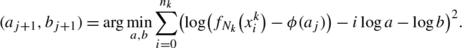
Given ϕ(a _j), the estimate of $f_{N_{k}}^{*}$, Step 2 of Subroutine B computes the rate of convergence coefficient that best fits $\{f_{N_{k}}(x_{i}^{k})\}_{i=0}^{n_{k}}$ in a least-square sense. Specifically, we use the regression model

$$ e(i) := a^ib $$

(41)

to estimate the distance $f_{N_{k}}(x_{i}^{k})-f_{N_{k}}^{*}$ after iteration i, where a and b are unknown regression coefficients estimated based on the data set $\{(i, f_{N_{k}}(x_{i}^{k})-\phi(a_{j}))\}_{i=0}^{n_{k}}$. Using a logarithmic transformation, we easily obtain the values of the transformed regression coefficients loga and logb by linear least-square regression; see (38). The corresponding values of a and b are denoted by a _j+1 and b _j+1.

Subroutine B is stated in [12] without any proof about its convergence. The authors’ incorrectly claim that it provides the correct rate of convergence θ given that the sequence $\{ f_{N_{k}}(x_{i}^{k})\}_{i=0}^{n_{k}}$ is exactly linear, i.e., equality holds in Assumption 1. While we find that Subroutine B yields reasonable estimates of the rate of convergence in numerical examples, the situation is more complicated than stated in [12] as the below analysis shows.

We view Subroutine B as a fixed-point iteration and adopt the following notation. Given the observations $\{f_{N_{k}}(x_{i}^{k})\}_{i=0}^{n_{k}}$, we view the calculations in Steps 1 and 2 of Subroutine B as a function g:ℝ→ℝ that takes as input an estimate a _j of the rate of convergence coefficient and returns another estimate a _j+1. We note that g(⋅) obviously depends on the observations $\{ f_{N_{k}}(x_{i}^{k})\}_{i=0}^{n_{k}}$ even though it is not indicated by the notation. The properties of g(⋅) explain the performance of Subroutine B as we see next. The proofs of the below results are given in the appendix due to their lengths. We first show that Steps 1 and 2 of Subroutine B are given by a relatively simple formula.

Proposition 2

Suppose that $\{f_{N_{k}}(x_{i}^{k})\}_{i=0}^{n_{k}}$, with n _k>1, satisfies $f_{N_{k}}(x_{i}^{k})> f_{N_{k}}(x_{i+1}^{k})$ for all i=0,1,…,n _k−1. Then, for any a∈(0,1),

$$ g(a) = \prod_{i=n_k^0}^{n_k} \biggl(\frac{f_{N_k}(x_i^k)-\phi (a)}{f_{N_k}(x_{n_k-i}^k)-\phi(a)} \biggr)^{\alpha_i}\in(0,1), $$

(42)

where $n_{k}^{0} := \lfloor n_{k}/2\rfloor+1$, with ⌊n _k/2⌋ being the largest integer no larger than n/2, $\alpha_{i} := 12(i-n_{k}/2)/(n_{k}^{3} + 3n_{k}^{2} + 2n_{k})$, and ϕ(a) is as in (37) with a _j replaced by a.

Proof

See Appendix. □

For notational convenience, we define g(0)=0 and g(1)=1. The next theorem states that Subroutine B converges to a fixed point of g(⋅), which implies that Subroutine B terminates after a finite number of iterations.

Theorem 4

Suppose that $\{f_{N_{k}}(x_{i}^{k})\}_{i=0}^{n_{k}}$, with n _k>1, satisfies $f_{N_{k}}(x_{i}^{k})>f_{N_{k}}(x_{i+1}^{k})$ for all i=0,1,…,n _k−1. For any a ₀∈(0,1), the sequence of iterates $\{a_{j}\}_{j=0}^{\infty}$ generated by the recursion a _j+1=g(a _j), j=0,1,2,…, converges to a fixed point a ^∗∈[0,1] of g(⋅), i.e., a ^∗=g(a ^∗). Moreover, if $\hat{\theta}_{k}\in(0,1)$, Subroutine B terminates in finite time for any ϵ _θ>0.

Proof

See Appendix. □

We observe that the assumptions in Proposition 2 and Theorem 4 are rather weak. Subroutine B is guaranteed to terminate when the algorithm map generates descent in the objective function value in each iteration, which is typical for standard nonlinear programming algorithms. If the sequence of function values $\{ f_{N_{k}}(x_{i}^{k})\}_{i=0}^{n_{k}}$ is exactly linear with rate of convergence coefficient $\theta_{N_{k}}\in(0,1)$, then $\theta_{N_{k}}$ is a fixed point of g(⋅) as stated in the follow theorem.

Theorem 5

Suppose that $\{f_{N_{k}}(x_{i}^{k})\}_{i=0}^{n_{k}}$, with n _k>1, satisfies $f_{N_{k}}(x_{i+1}^{k}) - f_{N_{k}}^{*} = \theta_{N_{k}}(f_{N_{k}}(x_{i}^{k}) - f_{N_{k}}^{*})$ for all i=0,1,2,… and some rate of convergence coefficient $\theta_{N_{k}}\in(0,1)$. Then, $\theta_{N_{k}} = g(\theta_{N_{k}})$.

Proof

See Appendix. □

In view of Theorems 4 and 5, we see that Subroutine B converges to a fixed point of g(⋅) and that the true rate of convergence coefficient is a fixed point of g(⋅) under the assumption of exact linear rate of convergence. Unfortunately, there may be more than one fixed point of g(⋅) and, hence, we cannot guarantee that Subroutine B converges to the rate of convergence coefficient from an arbitrary starting point. For example, if n _k=20, θ=0.15, and $f_{N_{k}}(x_{i}^{k}) = \theta^{i}$, i=1,2,…,n _k, with $f_{N_{k}}(x_{0}^{k}) = 1$, then Subroutine B converges to the correct value 0.15 if initialized with $\hat{\theta}_{k} \in(0,0.6633]$ and it converges to the incorrect value 0.8625 if initialized with $\hat{\theta}_{k} \in[0.6633, 1)$. (Here numbers are rounded to four digits.) The next theorem shows that Subroutine B indeed converges to the rate of convergence coefficient if initialized sufficiently close to that number for a wide range of values of $\theta_{N_{k}}$. In our numerical tests, we find that the range of sufficiently close starting points is typically rather wide as in the example given above. This experience appears consistent with that of [12].

Theorem 6

Suppose that $\{f_{N_{k}}(x_{i}^{k})\}_{i=0}^{n_{k}}$, with n _k>1, satisfies $f_{N_{k}}(x_{i+1}^{k}) - f_{N_{k}}^{*} = \theta_{N_{k}}(f_{N_{k}}(x_{i}^{k}) - f_{N_{k}}^{*})$ for all i=0,1,2,… and some rate of convergence coefficient $\theta_{N_{k}}\in(0,0.99]$. If Subroutine B has generated the sequence $\{a_{j}\}_{j=0}^{\infty}$, ignoring the stopping criterion in Step 3, with $a_{0}=\hat{\theta}_{k}$ sufficiently close to $\theta_{N_{k}}$, then $a_{j}\to\theta_{N_{k}}$, as j→∞.

Proof

See Appendix. □

It appears that Theorem 6 also holds for $\theta_{N_{k}}\in(0.99, 1)$. However, the verification of this requires a large computational effort as can be deduced from the proof of Theorem 6, which we have not carried out.

In view of Theorems 4, 5, and 6, we see that Subroutine B terminates in finite time under weak assumptions and it obtains the correct rate of convergence coefficient under somewhat stronger assumptions.

We next present a subroutine for estimating f ^∗ based on a weighted average of estimates of $f_{N_{l}}^{*}$, l=1,2,…,k. We let $\hat{f}_{k}^{*}$ and $\hat{\theta}_{k+1}$ denote the estimates of f ^∗ and θ, respectively, available prior to the execution of Subroutine C.

Subroutine C (Computes estimate $\hat{f}_{k+1}^{*}$ of the optimal value f ^∗)

Input. :: Previous optimal value estimate $\hat{f}_{k}^{*}$, estimate of rate of convergence coefficient $\hat{\theta}_{k+1}$, and function values from the current stage $\{f_{N_{k}}(x_{i}^{k})\}_{i=0}^{n_{k}}$.
Step 1. :: Compute an estimate of $f_{N_{k}}^{*}$:
$$ \hat{m}_k := \min_{i=0, 1, \ldots, n_k-1} \frac{f_{N_k}(x_{n_k}^k) - \hat{\theta}_{k+1}^{n_k-i}f_{N_k}(x_{i}^k)}{1-\hat{\theta}_{k+1}^{n_k-i}}. $$
(43)
Step 2. :: Compute
$$ \hat{f}_{k+1}^* := \frac{N_k}{\sum_{l=1}^{k} N_l} \hat{m}_k+ \frac{\sum_{l=1}^{k-1} N_l}{\sum_{l=1}^{k} N_l} \hat{f}_k^*. $$
(44)
Output. :: Optimal value estimate $\hat{f}_{k+1}^{*}$.

Step 1 of Subroutine C is the same as in [12] and in view of Lemma 1 provides a lower bound on $f_{N_{k}}^{*}$. The next result shows that $\hat{f}_{k+1}^{*}$, on average, is a lower bound on f ^∗ under certain assumptions. (Similar lower bounds on the optimal value are determined in [24, 28].) Using a lower bound, we tend to conservatively estimate the computational effort needed to reach a near-optimal solution of P.

Proposition 3

Suppose that $\{f_{N_{k}}(x_{i}^{k})\}_{i=0}^{n_{k}}$ satisfies $f_{N_{k}}(x_{i+1}^{k}) - f_{N_{k}}^{*} \leq\theta_{N_{k}}(f_{N_{k}}(x_{i}^{k}) - f_{N_{k}}^{*})$ for all i=0,1,2,… and some rate of convergence coefficient $\theta_{N_{k}}\in(0,1)$. If Subroutine C’s input $\hat{f}_{k}^{*}\leq f^{*}$ and $\hat{\theta}_{k+1}\geq\theta_{N_{k}}$, then $E[\hat{f}_{k+1}^{*}]\leq f^{*}$, where E denotes the expectation with respect to the random sample of stage k.

Proof

We deduce from Lemma 1 that $\hat{m}_{k} \leq f_{N_{k}}^{*}$ a.s. Hence, using the fact that $E[f_{N}^{*}] \leq f^{*}$ for all N∈ℕ, see, e.g., [24], we obtain that

(45)

□

Under stronger assumptions, we also determine the asymptotic distribution of $\hat{f}_{k+1}^{*}$.

Proposition 4

Suppose that Assumptions 3 and 4 hold, that P has a unique optimal solution x ^∗∈X, and that $\{f_{N_{l}}(x_{i}^{l})\}_{i=0}^{n_{l}}$, l=1,2,…,k, satisfy $f_{N_{l}}(x_{i+1}^{l}) - f_{N_{l}}^{*} = \theta_{N_{l}}(f_{N_{l}}(x_{i}^{l}) - f_{N_{l}}^{*})$ for some rate of convergence coefficients $\theta_{N_{l}}\in(0,1)$ and for all i=0,1,2,…,n _l−1 and l=1,2,…,k. Let $S_{k} = \sum_{l=1}^{k} N_{l}$. If Subroutine C is applied at stages l=1,2,…,k with inputs $\hat{f}_{l}$ from the previous stage and $\hat{\theta}_{l+1}\geq\theta_{N_{l}}$, then $S_{k}^{1/2}(\hat{f}_{k+1}^{*}-f^{*})\Rightarrow \mathcal {N}(0,\sigma^{2}(x^{*}))$, as S _k→∞.

Proof

See Appendix. □

In view of Proposition 4, $\hat{f}_{k+1}^{*}$ is approximately normally distributed with mean f ^∗ and variance $\sigma^{2}(x^{*})/\sum_{l=1}^{k} N_{l}$ for large sample sizes under the stated assumptions.

The next subroutine estimates the function value at the end of stage k.

Subroutine D (Computes estimate $f_{N^{*}}(x_{n_{k}}^{k})$ of $f(x_{n_{k}}^{k})$)

Input. :: Verification sample size N ^∗ and last iterate $x_{n_{k}}^{k}$.
Step 1. :: Generate an independent sample $\{\omega_{j}^{*}\}_{j=1}^{N^{*}}$ from ℙ.
Step 2. :: Compute the sample average
$$ f_{N^*}\bigl(x_{n_k}^k\bigr) = \frac{1}{N^*} \sum_{j=1}^{N^*} F\bigl(x_{n_k}^k, \omega_j^*\bigr). $$
(46)
Output. :: Function value estimate $f_{N^{*}}(x_{n_{k}}^{k})$.

Subroutine D uses the standard sample average estimator to estimate $f(x_{n_{k}}^{k})$. Under Assumption 3, the central limit theorem states that for a given $x_{n_{k}}^{k}\in \mathbb {R}^{d}$, $f_{N^{*}}(x_{n_{k}}^{k})$ is approximately normally distributed with mean $f(x_{n_{k}}^{k})$ and variance $\sigma^{2}(x_{n_{k}}^{k})/N^{*}$ for large N ^∗.

The next subroutine deals with the computational work parameters.

Subroutine E (Computes estimates of computational work parameters w and w ^∗)

Input. :: Time t _k required to compute iterates during stage k and time $t_{k}^{*}$ to verify the last function value of stage k as well as corresponding sample size N _k, iteration number n _k, and verification sample size N ^∗.
Step 1. :: Set p _w=t _k/(N _k n _k) and $p_{w}^{*} = t_{k}^{*}/N^{*}$.
Output. :: Estimated computational work parameters p _w and $p_{w}^{*}$.

Subroutine E estimates the computational work parameters w and w ^∗ in the computational work model (33) using two computing times observed during stage k. In principle, one could use past stage’s computing times as well, but the simple Subroutine E performs well in the present context with the estimated computational work parameters p _w and $p_{w}^{*}$ varying little from stage to stage in numerical tests.

Subroutines C and D do not guarantee that $\hat{f}_{k+1}^{*}\leq f_{N^{*}}(x_{n_{k}}^{k})$, i.e., that the optimal value estimate is no larger than the estimated current objective function value. That inequality may be violated in early stages when estimates of f ^∗ could be poor. These estimates are intended to be used in $\mathbf{S\mbox{-}SSCP}_{k+1}$ and an estimated current function value that is within ϵ of the estimated optimal value would result in a trivial instance of $\mathbf{S\mbox{-}SSCP}_{k+1}$: the optimal number of iterations for stage k+1 would be zero since the terminal surrogate state is already reached. To avoid to some extent such trivial instances of $\mathbf{S\mbox{-}SSCP}_{k+1}$ prematurely, we adopt the following subroutine that makes adjustments to the estimates when needed.

Subroutine F (Sets estimates p _f and p ^∗, and gives surrogate optimality status)

Input. :: Estimates $\hat{f}_{k+1}^{*}$, $f_{N^{*}}(x_{n_{k}}^{k})$, and p _σ, verification sample size N ^∗, total sample size $\sum_{l=1}^{k} N_{l}$, and stopping tolerance ϵ.
Step 1. :: If $\hat{f}_{k+1}^{*} + \epsilon< f_{N^{*}}(x_{n_{k}}^{k})$, then set $p_{f} = f_{N^{*}}(x_{n_{k}}^{k})$ and $p^{*} = \hat{f}_{k+1}^{*}$, and surrogate optimality status to “suboptimal.” Else set $p_{f} = f_{N^{*}}(x_{n_{k}}^{k}) + p_{\sigma}/\sqrt{N^{*}}$ and $p^{*} = \hat{f}_{k+1}^{*} - p_{\sigma}/\sqrt{\sum_{l=1}^{k} N_{l}}$. If p ^∗+ϵ<p _f, set surrogate optimality status to “suboptimal.” Otherwise set surrogate optimality status to “optimal.”
Output. :: Surrogate optimality status and parameter estimates p _f and p ^∗.

Subroutine F sets $p_{f} = f_{N^{*}}(x_{n_{k}}^{k})$ and $p^{*} = \hat{f}_{k+1}^{*}$, when the estimates $f_{N^{*}}(x_{n_{k}}^{k})$ and $\hat{f}_{k+1}^{*}$ appear “reasonable” in the sense that the current estimates predict that a terminal surrogate state is not reached. In contrast, if $\hat{f}_{k+1}^{*} + \epsilon\geq f_{N^{*}}(x_{n_{k}}^{k})$, i.e., a near-optimal solution appears to be reached, then Subroutine F replaces the estimates $f_{N^{*}}(x_{n_{k}}^{k})$ and $\hat{f}_{k+1}^{*}$ by more conservative estimates. Specifically, $p_{\sigma}/\sqrt{N^{*}}$ is added to $f_{N^{*}}(x_{n_{k}}^{k})$ and $p_{\sigma}/\sqrt{\sum_{l=1}^{k} N_{l}}$ is subtract off $\hat{f}_{k+1}^{*}$, which both represent shifting one standard deviation in the respective directions; see Proposition 4 and the discussion after Subroutine D. If either the original parameter estimates or the conservative ones predict that a near-optimal solution is not reached, we label the current solution “suboptimal” according to the surrogate model. Of course, a truly near-optimal solution may be labeled “suboptimal” due to the uncertainty and approximations in the surrogate model. If both the original and the conservative estimates predict a near-optimal solution, we label the situation “optimal.” Again, we stress that this does not imply that the current solution is nearly optimal. It merely indicates that the surrogate model has reached the terminal surrogate state and can therefore not be used to generate a sample size and a number of iterations for the next stage. In this case, as we see in the statement of Algorithm 2 below, we resort to a default policy for determining sample size and number of iterations.

4.2 Initialization subroutine

The final subroutine determines parameters for $\mathbf{S\mbox{-}SSCP}_{1}$, the first surrogate sample-size control problem to be solved at the beginning of Stage 1 of Algorithm 2.

Subroutine 0 (Computes initial parameter estimates p _f, p ^∗, and p _σ)

Input. :

Initial sample size N ₀ and initial iterate $x_{0}^{0}$.

Step 1. :

Generate an independent sample $\{\omega_{j}^{0}\}_{j=1}^{N_{0}}$ from ℙ.

Step 2. :

Compute the sample average

$$ f_{N_0}\bigl(x_0^0\bigr) = \frac{1}{N_0} \sum_{j=1}^{N_0} F\bigl(x_{0}^0, \omega_j^0\bigr) $$

(47)

and corresponding variance estimate

$$ \hat{\sigma}^2_{1} = \frac{1}{N_0-1} \sum_{j=1}^{N_0} \bigl(F\bigl(x_0^{0}, \omega_j^0\bigr) - f_{N_{0}}\bigl(x_{0}^{0} \bigr)\bigr)^2. $$

(48)

Step 3. :

Set $p_{f} = f_{N_{0}}(x_{0}^{0}) + \hat{\sigma}_{1}/\sqrt {N_{0}}$, $p^{*} = \min\{0, f_{N_{0}}(x_{0}^{0})-1\}$, and $p_{\sigma}= \hat{\sigma}_{1}$.

Output. :

Parameter estimates p _f, p ^∗, and p _σ.

Step 3 of Subroutine 0 computes a likely conservative estimate of $f(x_{0}^{0})$ by adding one standard deviation to the unbiased estimate $f_{N_{0}}(x_{0}^{0})$. Step 3 also computes a rudimentary estimate of f ^∗. If problem specific information is available, the initial estimate of f ^∗ may be improved.

4.3 Full algorithm

Combining $\mathbf{S\mbox{-}SSCP}_{k}$ and the above subroutines with Algorithm 1, we obtain Algorithm 2. Below, we indicate in parenthesis after a subroutine name the input parameters used in that subroutine.

Algorithm 2

(Adaptive algorithm for P)

Data. :: Optimality tolerance ϵ>0; initial sample size N ₀∈ℕ; verification sample size N ^∗; default sample size factor γ _N>0; default iteration number γ _n∈ℕ; smoothing parameter α _θ∈[0,1]; initial estimate of rate of convergence coefficient $\hat{\theta}_{1}$; initial solution $x_{0}^{0} \in X$; initial estimate of work coefficients p _w and $p_{w}^{*}$.
Step 0. :: Run Subroutine 0($N_{0}, x_{0}^{0}$) to obtain p _f, p ^∗, and p _σ. Set $p_{\theta}= \hat{\theta}_{1}$, $x_{0}^{1} = x_{0}^{0}$, and stage counter k=1.
Step 1a. :: Solve $\mathbf{S\mbox{-}SSCP}_{k}(p_{f},p^{*},p_{\theta},p_{\sigma},p_{w},p_{w}^{*},\epsilon)$ to obtain N _k and n _k.
Step 1b. :: Generate an independent sample $\{\omega^{k}_{j}\}_{j=1}^{N_{k}}$ from ℙ.
Step 2. :: For i=0 to n _k−1: Compute $x_{i+1}^{k} = A_{N_{k}}(x_{i}^{k})$ using the sample generated in Step 1b. Let t _k denote the time to compute these iterates.
Step 3a. :: Run $\mathbf{Subroutine A}(x_{n_{k}}^{k}, \{\omega^{k}_{j}\}_{j=1}^{N_{k}})$ to obtain p _σ.
Step 3b. :: Run $\mathbf{Subroutine B}(\hat{\theta}_{k},\{ f_{N_{k}}(x_{i}^{k})\}_{i=0}^{n_{k}})$ to obtain $\hat{\theta}$, and set $\hat{\theta}_{k+1} = \alpha_{\theta}\hat{\theta}+ (1-\alpha_{\theta})\hat{\theta}_{k}$ and $p_{\theta}= \hat{\theta}_{k+1}$.
Step 3c. :: Run $\mathbf{Subroutine C}(\hat{f}_{k}^{*},\hat{\theta}_{k+1},\{f_{N_{k}}(x_{i}^{k})\}_{i=0}^{n_{k}})$ to obtain $\hat{f}_{k+1}^{*}$.
Step 3d. :: Run $\mathbf{Subroutine D}(N^{*}, x_{n_{k}}^{k})$ to obtain $f_{N^{*}}(x_{n_{k}}^{k})$. Let $t^{*}_{k}$ be the time required to run this subroutine.
Step 3e. :: Run $\mathbf{Subroutine E}(t_{k}, t_{k}^{*},N_{k},n_{k},N^{*})$ to obtain p _w and $p_{w}^{*}$.
Step 3f. :: Run $\mathbf{Subroutine F}(\hat{f}_{k+1}^{*}, f_{N^{*}}(x_{n_{k}}^{k}), p_{\sigma}, N^{*}, \sum_{l=1}^{k} N_{l}, \epsilon)$ to obtain surrogate optimality status and parameter estimates p _f and p ^∗. Set $x_{0}^{k+1}=x_{n_{k}}^{k}$, replace k by k+1. If surrogate optimality status is “suboptimal,” then go to Step 1a. Else (surrogate optimality status is “optimal”), set N _k=⌈γ _N N _k−1⌉ and n _k=γ _n and go to Step 1b.

In Step 3b of Algorithm 2, the estimated rate of convergence coefficient is modified in view of previous estimates using exponential smoothing. Consequently, we avoid large fluctuations in this estimate. In Step 3f, Algorithm 2 resorts to a default policy defined by the parameters γ _N and γ _n when the surrogate sample-size control problem believes the current iterate satisfies the required tolerance.

Algorithm 2 is identical to Algorithm 1 except that the sample sizes and numbers of iterations are selected in a particular manner using $\mathbf{S\mbox{-}SSCP}_{k}$. The underlying probability space $\bar{\varOmega}$ of Algorithm 1 is also augmented with $\varOmega^{N^{*}}\times\varOmega^{N^{*}}\times\ldots$ for Algorithm 2 to account for the verification sample size; see Subroutine D. Since this change in probability space is trivial to account for in Theorem 1, it follows that if the assumptions of that theorem are satisfied, then Algorithm 2 converges almost surely to a near-optimal solution. We note that it is straightforward to impose restrictions on the values of $\{N_{k},n_{k}\}_{k=1}^{\infty}$ in $\mathbf{S\mbox{-}SSCP}_{k}$ required by Theorem 1 through the construction of the sets D _N and D _n.

5 Computational studies

In this section, we examine numerically the S-SSCP policy and compare it with practical alternatives, including the asymptotically optimal policy of the recent paper [30]. Specifically, we compare the computing time required to obtain a near-optimal solution by Algorithm 2 using different sample-size selection policies in Step 1a. As mentioned in Sect. 1, stochastic programs may also be solved by algorithms not based on SAA and VSAA. However, in this paper we do not compare across algorithmic frameworks and focus on efficient sample-size selection within VSAA when applied to smooth stochastic programs.

We implement Algorithm 2 in Matlab Version 7.4 and run the calculations on a laptop computer with 2.16 GHz processor, 2 GB RAM, and Windows XP operating system, unless otherwise stated. We use one iteration of the projected gradient method with Armijo step size rule (see, e.g., p. 67 of [33]) as the algorithm map A _N(⋅). The quadratic direction finding problem in the projected gradient method is solved using LSSOL [10] as implemented in TOMLAB 7.0 [14].

In all computational tests, we use parameters α=0.5 and β=0.8 in Armijo step size rule (see p. 67 of [33]) as well as exponential smoothing parameter α _θ=1/3 in Step 3b of Algorithm 2 and tolerance ϵ _θ=0.0001 in Subroutine B. We use initial sample size N ₀=1000, default sample size factor γ _N=1.1, default iteration number γ _n=3, and initial estimate of rate of convergence coefficient $\hat{\theta}_{1}=0.9$. Our initial computational work parameters p _w and $p_{w}^{*}$ are 3 and 1, respectively.

5.1 Numerical examples

We consider the following four problem instances. The first instance is a constructed example of P with known optimal solution. The second instance arises in investment portfolio optimization, the third in military and civilian search and rescue operations, and the fourth in engineering design with multiple performance functions. The second and fourth problem instances illustrate that Algorithm 2 may be used even if F(⋅,ω) is nonsmooth, when proper approximations are used.

5.1.1 Problem instance QUAD

Problem instance QUAD is defined in terms of

$$ F(x,\omega) = \sum_{i=1}^{20} a_i(x_i-b_i\omega_i)^2 $$

(49)

with b _i=21−i, i=1,2,…,20, and ω=(ω ₁,ω ₂,…,ω ₂₀)′ being a vector of 20 independent and [0,1]-uniformly distributed random variables. We use the values a _i=i, i=1,2,…,20. (We have also examined other values for a _i and obtained similar results to those reported below.) The instances are unconstrained and we set X equal to a sufficiently large convex compact subset of ℝ²⁰ that includes all relevant solutions. Obviously, QUAD is strongly convex with a unique global minimizer $x^{*}=(x_{1}^{*}, \ldots, x_{20}^{*})'$, where $x_{i}^{*} = b_{i}/2$. The optimal value is $\sum_{i=1}^{20} a_{i} b_{i}^{2}/12$. Even though solvable without VSAA, we use this simple problem instance to illustrate our approach. We set $x_{0}^{0} = 0\in \mathbb {R}^{20}$ and use relative optimality tolerance 0.001, i.e., ϵ=0.001p ^∗ in Algorithm 2.

5.1.2 Problem instance PORTFOLIO

The second problem instance, PORTFOLIO, is taken from [22] and arises in optimization of investment portfolios. We consider d−1 financial instruments with random returns given by the (d−1)-dimensional random vector $\omega= \bar{R} + Qu$, where $\bar{R} = (\bar{R}_{1}, \bar{R}_{2}, \ldots, \bar{R}_{d-1})'$, with $\bar{R}_{i}$ being the expected return of instrument i, Q is an (d−1)-by-(d−1) matrix, and u is a standard normal (d−1)-dimensional random vector. As in [22], we randomly generate $\bar{R}$ using an independent sample from a uniform distribution on [0.9,1.2] and Q using an independent sample from a uniform distribution on [0,0.1]. The goal is to distribute one unit of wealth across the d−1 instruments such that the Conditional Value-at-Risk of the portfolio return is minimized and the expected portfolio return is no smaller than 1.05. We let x _i∈ℝ denote the amount of investment in instrument i, i=1,2,…,d−1. This results in the objective function (see [22, 36])

$$ f(x) = \mathbb {E}\Biggl[x_d + \frac{1}{1-t}\max \Biggl\{-\sum_{i=1}^{d-1} \omega_ix_i - x_d, 0 \Biggr\} \Biggr], $$

(50)

where x=(x ₁,x ₂,…,x _d)′, with x _d∈ℝ being an auxiliary decision variable, and t∈(0,1) is a probability level. The feasible region

$$ X = \Biggl\{x\in \mathbb {R}^d\Biggm{\vert} \sum_{i=1}^{d-1} x_i = 1,\ \sum_{i=1}^{d-1} \bar{R}_ix_i \geq1.05,\ x_i\geq0,\ i = 1, 2, \ldots, d-1 \Biggr\}. $$

(51)

We use d=101 and t=0.9.

The expression inside the expectation in (50) is not continuously differentiable everywhere for ℙ-almost every ω∈Ω. We overcome this difficulty by smoothing that expression using exponential smoothing with smoothing parameter 10³; see [1, 31, 37, 52] for other applications of this approach as well as associated theory. This results in an error in function evaluation due to smoothing of less than 7×10⁻⁴ for all x∈ℝ¹⁰¹ and ω∈ℝ¹⁰⁰. This problem instance illustrates that also nonsmooth problems may be solved approximately by Algorithm 2. Of course, as pointed out in [22], this instance of P can be reformulated as a conic-quadratic programming problem and solved directly without the use of VSAA. Hence, this is a convenient test instance as we are able to verify using cvx [11] that the solutions obtained by Algorithm 2 are indeed nearly optimal.

We use initial solution $x_{0}^{0}=(0, 0, \ldots, 0, 1, 0, 0,\ldots, 0, -1)'$, where the 65-th component equals 1. In our data, the 65-th instrument has the largest expected return. Hence, the initial solution is the one with the largest expected portfolio return. We also set ϵ=0.05p ^∗. We implement this problem instance in Matlab Version 7.9 and run the calculations on a laptop computer with 2.26 GHz processor, 3.5 GB RAM, and Windows XP operating system.

5.1.3 Problem instance SEARCH

The next problem instance generalizes a classical problem arising in search and detection applications. Consider an area of interest divided into d cells. A stationary target is located in one of the cells. A priori information gives that the probability that the target is in cell i is p _i, i=1,2,…,d, with $\sum_{i=1}^{d} p_{i} = 1$. The goal is to optimally allocate one time unit of search effort such that the probability of not detecting the target is minimized (see, e.g., p. 5-1 in [51]). We generalize this problem and consider a random search effectiveness in cell i per time unit. We let x=(x ₁,x ₂,…,x _d)′∈ℝ^d, with x _i representing the number of time units allocated to cell i, and let ω=(ω ₁,ω ₂,…,ω _d)′, with ω _i, i=1,2,…,d, being independent lognormally distributed random variables (with parameters ξ _i=100u _i and λ _i=0, where u _i∈(0,1) are given data generated by independent sampling from a uniform distribution) representing the random search effectiveness in cell i. Then, the probability of not detecting the target is $f(x) = \mathbb {E}[F(x,\omega)]$, where

$$ F(x,\omega) = \sum_{i=1}^{d} p_i e^{-\omega_i x_i}. $$

(52)

The decision variables are constrained by $\sum_{i=1}^{d} x_{i} = 1$ and x _i≥0, i=1,2,…,d. We consider d=100 cells. This problem instance, referred to as SEARCH, is convex. We observe that the expectation in the objective function can be computed by (numerically) solving d one-dimensional integrals. However, our goal is to illustrate Algorithm 2, which is based on VSAA, so we do not pursue that avenue. For this problem instance, we use $x_{0}^{0} = (1/100, \ldots, 1/100)'\in \mathbb {R}^{100}$ and use relative optimality tolerance 0.001, i.e., ϵ=0.001p ^∗ in Algorithm 2.

5.1.4 Problem instance TRUSS

The last problem instance deals with the design of a truss structure with topology given in Fig. 2. The truss is subject to a random load L in its mid-span. L is lognormally distributed with mean 100 kN and standard deviation 10 kN. Let S _i be the yield stress of member i. Members 1–7 have lognormally distributed yield stresses with means 100, 120, 180, 190, 200, 210, and 220 N/mm², respectively. Members 1 and 2 have standard deviation 5 N/mm² and members 3–7 have standard deviations 10 N/mm². The yield stresses of members 1 and 2 are correlated with correlation coefficients 0.8. However, their correlation coefficients with the other yield stresses are 0.5. Similarly, the yield stresses of members 3–7 are correlated with correlation coefficients 0.8, but their correlation coefficients with the yield stresses of members 1 and 2 are 0.5. The load L is independent of the yield stresses.

The design vector x=(x ₁,x ₂,…,x ₇)′∈ℝ⁷, where x _i is the cross-section area (in 1000 mm²) of member i. The truss fails if any of the members exceed their yield stress and, hence, the probability of failure is $P[\bigcup_{i=1}^{7} \{S_{i}x_{i} - L/\zeta_{i}\leq0\}]$, where $\zeta_{i} = 1/(2\sqrt{3})$ for i=1,2, and $\zeta_{i} = 1/\sqrt{3}$ for i=3,4,…,7 (see [40] for details). Using the approach in [40], see also [39], we find that this probability of failure can be approximated with high accuracy by

$$ f(x) = \mathbb {E}\Bigl[ \max\Bigl\{\rho, \max_{i=1,\ldots,7} \bigl\{1- \chi^2_8\bigl(r_i^2(x,\omega) \bigr)\bigr\}\Bigr\}\Bigr] $$

(53)

where ρ>0 is an approximation parameter set equal to 20, $\chi^{2}_{8}(\cdot)$ is the Chi-square cumulative distribution function with 8 degrees of freedom, ω is an eight-dimensional random vector of independent standard normal random variables obtained from the original random variables (L,S ₁,…,S ₇) using a Nataf probability transformation, and r _i(⋅,ω) is a smooth distance function. The function (53) is of form (1) and is continuously differentiable under moderate assumptions [39]. As in the case of PORTFOLIO, the expression inside the brackets in (53) is not continuously differentiable everywhere for ℙ-almost every ω∈Ω. We again overcome this difficulty by smoothing that expression using exponential smoothing with smoothing parameter 10⁷; see [35]. This results in an error in function evaluation due to smoothing of less than 2×10⁻⁷ for all x∈ℝ⁷ and ω∈Ω. As the problem instance is not known to be convex, it illustrates that the proposed approach may be effective in such cases too. The goal in this design problem, denoted TRUSS, is to minimize f(x) subject to $\sum_{i=1}^{7} x_{i} = 3$, x _i≤0.5, x _i≥0.2, i=1,2,…,7. We use $x_{0}^{0} = (3/7, \ldots, 3/7)'\in \mathbb {R}^{7}$ and ϵ=0.05p ^∗.

5.2 Computational results

We apply Algorithm 2 with different sample-size selection policies to the four problem instances. The measure of performance of a policy is the computing time in Algorithm 2 until the first time a stage k satisfies

$$ \biggl[0, \max \biggl\{f_{N^*} \bigl(x_{n_k}^k\bigr) - \hat{f}^*_{k+1} + z_{1-\alpha _s}p_\sigma\sqrt{\frac{1}{N^*}+ \frac{1}{\sum_{l=1}^k N_l}}, 0 \biggr\} \biggr]\subset[0, \epsilon] $$

(54)

at the end of the stage. Here, ϵ>0 is the required tolerance and $z_{1-\alpha_{s}}$ is the 1−α _s quantile of the standard normal cumulative distribution function. We use α _s=0.05 in our tests. The left-hand side in (54) is motivated as follows.

For a given x∈ℝ^d, $f_{N^{*}}(x)$ and $\hat{f}^{*}_{k+1}$ are independent when the sample used to compute $f_{N^{*}}(x)$ is independent of those used to compute $\hat{f}^{*}_{k+1}$. Hence, in view of Proposition 4 and the discussion after Subroutine D, $f_{N^{*}}(x)-\hat{f}^{*}_{k+1}$ is approximately normally distributed with mean f(x)−f ^∗ and variance $\sigma^{2}(x)/N^{*} + \sigma^{2}(x^{*})/\sum_{l=1}^{k} N_{l}$ for large N ^∗ and $\sum_{l=1}^{k} N_{l}$. Consequently, $[0, \max\{f_{N^{*}}(x) - \hat{f}^{*}_{k+1} + z_{1-\alpha_{s}}\sqrt{\sigma^{2}(x)/N^{*}+\sigma^{2}(x^{*})/\sum_{l=1}^{k} N_{l}}, 0\}]$ is an approximate 100(1−α _s) % confidence interval for f(x)−f ^∗. We include the max-operator in the expression for this interval as f(x)−f ^∗≥0 for any x∈X. The assumptions underlying this confidence interval are not fully satisfied in the context of Algorithm 2 for three reasons. First, σ(x) and σ(x ^∗) are assumed known, which may not be the case. Second, since we are interested in $x = x_{n_{k}}^{k}$, the final iterate of the k-th stage, and $x_{n_{k}}^{k}$ is generated using the same samples as those underlying $\hat{f}^{*}_{k+1}$, $f_{N^{*}}(x_{n_{k}}^{k})$ and $\hat{f}^{*}_{k+1}$ may not be independent. Third, we check the confidence interval after the completion of each stage in Algorithm 2, which implies sequential testing that may introduce a bias not accounted for in the confidence interval. In spite of these facts, we heuristically adopt the confidence interval with σ(x) and σ(x ^∗) replaced by the standard deviation estimate p _σ as the basis for our stopping criterion, which leads to (54). Consequently, we cannot guarantee that the left-hand side in (54) attains the stipulated coverage probability. However, we find empirically that the coverage probabilities are satisfactory. Specifically, Algorithm 2 stops, using (54), with an $x_{n_{k}}^{k}$ that fails to satisfy $f(x_{n_{k}}^{k})-f^{*}\leq\epsilon$ in only 1 % of 320 independent runs on QUAD, which is well within the 5 % indicated by the confidence level 0.95. While not tested as comprehensively, the stopping criterion performs well also on the other problem instances. On PORTFOLIO, the stopping criterion never stops prematurely on 82 runs. It stops prematurely 1 time out of 90 and 0 times out of 90 for SEARCH and TRUSS, respectively, also well within he requested 5 %.

The proximity to optimality of a solution obtained by Algorithm 2 could also be estimated using an optimality function [37], a hypothesis test of Karush-Kuhn-Tucker conditions [47], or an optimality gap estimate based on replications [24, 28]. However, we do not pursue those avenues here as (54) appears sufficient for our purpose of compare different sample-size selection policies.

In view of (54) and the fact that α _s=0.05, we select N ^∗ so that the variability in $f_{N^{*}}(x_{n_{k}}^{k})$ is relatively small. Hence, we set $N^{*} = \lceil (\hat{\sigma}_{1} z_{0.95}/(\epsilon/2))^{2}\rceil$, which is the smallest sample size that ensures that (54) is satisfied when $f_{N^{*}}(x_{n_{k}}^{k})-\hat{f}^{*}_{k+1} = \epsilon/2$ and there is no uncertainty in $f^{*}_{k+1}$, i.e., $\sum_{l=1}^{k} N_{l}$ “equals” infinity.

We start by examining the computational effort required to solve $\mathbf{S\mbox{-}SSCP}_{k}$ in Step 1a of Algorithm 2. As discussed in Sect. 3.3, that computational effort depends on the number of stages s, number possible sample sizes d _N, number of possible stage durations d _n, and number of discrete states d _f considered in $\mathbf{S\mbox{-}SSCP}_{k}$. Table 1 gives total computing times in seconds to solve $\mathbf{S\mbox{-}SSCP}_{k}$, $k= 1, 2, \ldots, k_{\epsilon}^{*}$, in Algorithm 2, where $k_{\epsilon}^{*}$ is the first stage satisfying the stopping criterion (54), for different values of s, d _N, d _n, and d _f when applied to QUAD (columns 6–7), PORTFOLIO (columns 8–9), SEARCH (columns 10–11), and TRUSS (columns 12–13). Termination occurs typically with $k_{\epsilon}^{*}$ between 5 and 15. The total computing times are averages over 10 independent runs and given in columns 6, 8, 10, and 12, with corresponding standard deviations given in columns 7, 9, 11, and 13. (The shorter times for PORTFOLIO are, in part, due to a faster computer.) Row 3 presents results for “high” values of s, d _N, d _n, and d _f as specified in columns 2–5 and we find the corresponding total computing times to be relatively long. Row 4 gives total computing times for a “medium” case with fewer discrete states d _f, which results in a reduction in the total computing time with a factor of about four. Row 5 considers the case with “low” values of s, d _N, d _n, and d _f. In this case, the total computing times for solving $\mathbf{S\mbox{-}SSCP}_{k}$, $k= 1, 2, \ldots, k_{\epsilon}^{*}$, is reduced with a factor of approximately 10–30 and amounts to only about one second per solution of the surrogate sample-size control problem. The results for all problem instances correspond closely with what is predicted by the complexity result $O(sd_{N}d_{n}d_{f}^{2})$ for $\mathbf{S\mbox{-}SSCP}_{k}$; see Sect. 3.3. We next examine how different values of s, d _N, d _n, and d _f influence the quality of the resulting S-SSCP policy.

Table 1 Total computing times (seconds), over all stages, to solve $\mathbf{S\mbox{-}SSCP}_{k}$ in Step 1a of Algorithm 2 with stopping criterion (54) for different values of s, d _N, d _n, and d _f. The times in columns 6, 8, 10, and 12 are averages over ten runs of Algorithm 2 when applied to QUAD, PORTFOLIO, SEARCH, and TRUSS, respectively. Standard deviations across the ten runs are listed in columns 7, 9, 11, and 13

Full size table

Using the same 10 independent runs of Algorithm 2 as in Table 1, rows 3–5 of Table 2 give the average computing times in seconds over the 10 runs for Algorithm 2 applied to QUAD and PORTFOLIO, excluding the time of Step 1a to solve $\mathbf{S\mbox{-}SSCP}_{k}$. (The remaining rows of Table 2 are discussed below.) Standard deviations of the times are given in columns 5 and 7. We find only a moderate variability across rows 3–5 in Table 2 and no clear indication that larger values of s, d _N, d _n, and d _f yield significantly better policies than smaller values.

Table 2 Average and standard deviation of computing times (seconds) over ten runs of Algorithm 2 excluding the time of Step 1a when applied to QUAD and PORTFOLIO. Averages are only over runs completed within 3600 seconds. If less than 10 runs finished within that time limit, we report the number that did finish in brackets

Full size table

Table 3 presents similar results as Table 2, but for problem instances SEARCH and TRUSS. Using the same 10 independent runs of Algorithm 2 as in Table 1, rows 3–5 of Table 3 present the average computing times in seconds over the 10 runs for Algorithm 2 excluding the time of Step 1a to solve $\mathbf{S\mbox{-}SSCP}_{k}$. Again, there is only a moderate variability in computing times across rows 3–5 in Table 3 and no clear indication that larger values of s, d _N, d _n, and d _f yield significantly better policies than smaller values. The results of rows 3–5 in Tables 2 and 3 as well as those of tests with other values of s, d _N, d _n, and d _f not reported here, indicate that relatively small values of s, d _N, d _n, and d _f may be sufficient to generate reasonable S-SSCP policies. In view of Table 1, small values of s, d _N, d _n, and d _f result in essentially negligible computing times for $\mathbf{S\mbox{-}SSCP}_{k}$. We anticipate that in real-world application of Algorithm 2 the main iterations of Step 2 in Algorithm 2 would require a significant amount of time, much more than the times for the present problem instances, due to large number of iterations, large sample sizes, and/or expansive function and gradient evaluations. In contrast, the total computing times to solve $\mathbf{S\mbox{-}SSCP}_{k}$ would remain about the same as they are essentially independent of the application. They only depend on the values of s, d _N, d _n, and d _f. Hence, we conjecture that the time to obtain the S-SSCP policy is negligible in many applications.

Table 3 Average and standard deviation of computing times (seconds) over ten runs of Algorithm 2 excluding the time of Step 1a when applied to SEARCH and TRUSS. Averages are only over runs completed within 15000 seconds. If less than 10 runs finished within that time limit, we report the number that did finish in brackets

Full size table

We next compare the S-SSCP policy with other reasonable alternatives. Rows 6–8 of Table 2 give times on QUAD and PORTFOLIO for an “additive policy” where N ₁=N ^∗/1000 and N _k=N ₁+(N ^∗−N ₁)k/20, k=2,3,…, with n _k=5,10, and 20, respectively, rows 9–11 give times for a “multiplicative policy” where N ₁=N ^∗/1000 and N _k=1.5^k−1 N ₁, k=2,3,…, with n _k=5,10, and 20, respectively, and rows 12–14 give times for the same multiplicative policy as the previous rows except that N _k=2^k−1 N ₁, k=2,3,…. Rows 15–17 report results for a fixed policy with N _k=N ^∗/2 and n _k=5 for all k. In Table 2 and elsewhere we indicate in brackets the number of terminations within a time limit, here one hour, when less than 10. Rows 18–29 follow policies deduced from the recommendation in [30]. Specifically, from an N ₁ given in column 3, N _k=1.1^k−1 N ₁, k=2,3,…, for rows 18–23 and N _k=1.5^k−1 N ₁, k=2,3,…, for rows 24–29. The number of iterations carried out at each stage is determined adaptively. For QUAD, which is unconstrained, the stage ends when the estimated distance $\|(\nabla^{2} f_{N_{k}}(x^{k}_{i}))^{-1}\nabla f_{N_{k}}(x^{k}_{i})\|$ to an optimal solution is no greater than $K/\sqrt{N_{k}}$ as recommended in [30]. For constrained problems such as PORTFOLIO, no recommendation is given and we use the distance between the current solution and a minimizer over X of a quadratic model of $f_{N_{k}}(\cdot)$ at the current solution as an estimate of the distance to an optimal solution. Column 2 of rows 18–29 gives values of K. The policies of rows 18–29 are asymptotically optimal in a sense defined in [30]. We note that N ^∗/1000 is typically around 600 and 100 for QUAD and PORTFOLIO, respectively. In all cases, N _k is set to 3,000,000, if the above policies propose a sample size of larger than 3,000,000.

We see from Table 2 that the S-SSCP policies are often significantly better than the alternative ones for both problem instances. The first additive policy on QUAD (see row 6 of Table 2) appears to be reasonably efficient and competitive with S-SSCP medium. On PORTFOLIO, the three additive policies are competitive. Other alternative policies, however, may require as much as an order of magnitude more computing time. The alternative policies deduced from the recommendation in [30] (see rows 18–29 in Table 2) may result in poor computing times, especially for PORTFOLIO where only two instances solve within the time limit. It appears that the policies in [30] have a tendency to “over-solve” each stage. This follows as a consequence from the difficulty of accurately estimating the distance to an optimal solution.

Table 4 gives estimates of the value of f(⋅) at the final iterate of Algorithm 2 for the interesting cases in Table 2 using an independent sample of size 500,000, which result in small estimator errors (95 % confidence interval halfwidth of 0.8 and 0.002 for QUAD and PORTFOLIO, respectively). We report both average estimates over the 10 runs (columns 4 and 6) as well as standard deviations (columns 5 and 7). Since f ^∗+ϵ equals 1348.8 for QUAD and −0.335 for PORTFOLIO, Table 4 indicates that all the cases that terminated by (54) return solutions within the required tolerance. On PORTFOLIO, not all policies terminate within one hour, but we still report the estimated function values at that time.

Table 4 Average and standard deviation of estimated objective function values over ten runs of Algorithm 2 for QUAD and PORTFOLIO

Full size table

Table 5 presents examples of sample sizes and number of iterations for QUAD for five runs using policies from Table 2. Columns 2–3 show that the policy S-SSCP high requires six stages and that the number of iterations tends to decrease as the stages progress. $\mathbf{S\mbox{-}SSCP}_{k}$ identifies this as a computationally efficient approach as the later stages necessarily would require a large sample size. We note that in QUAD N ^∗ is about 6×10⁵. Columns 4–5 shows comparable results for the additive policy with n _k=5 and N ₁=N ^∗/1000. The fixed increase in sample size after each stage appears to be to large in this case as the sample size reaches unnecessarily high values. The situation is similar for the multiplicative policy with factor 2, n _k=10, and N ₁=N ^∗/1000; see columns 6–7. For the multiplicative policies with factor 1.1, K=1, and N ₁=100 (columns 8–9) and with factor 1.5, K=1, and N ₁=N ^∗/1000 (columns 10–11), we find that the adaptive rule for determining the number of iterations for each stage tends to result in high values of n _k. Hence, the algorithm “over-solves” each stage, which may result in long computing times. Also, the number of stages may become excessive if the multiplicative factor is small; see columns 8–9. We observe similar behaviors to those in Table 5 for the other problem instances.

Table 5 Examples of sample sizes N _k and numbers of iterations n _k for QUAD in policies S-SSCP high (columns 2–3), Additive with n _k=5 and N ₁=N ^∗/1000 (columns 4–5), Multiplicative with factor 2, n _k=10, and N ₁=N ^∗/1000 (columns 6–7), Multiplicative with factor 1.1, K=1, and N ₁=100 (columns 8–9), and Multiplicative with factor 1.5, K=1, and N ₁=N ^∗/1000 (columns 10–11)

Full size table

Returning to Table 3, we see that also in the case of SEARCH and TRUSS the alternative policies perform poorly. Here, we do not examine the policies from [30] due to their poor performance in Table 2. On SEARCH, the S-SSCP policies appear to be the fastest, but one additive policy (row 6) and one multiplicative policy (row 12) are competitive. On the problem instance TRUSS (see columns 6 and 7 of Table 3), the S-SSCP policies again outperform most alternative policies with two additive policies (rows 6 and 7) being competitive. The fastest additive policy on average, however, has a larger standard deviations (coefficient of variations of roughly 1.1) than that of the S-SSCP policies (coefficient of variation of 0.7 on average). Hence, the user of that additive policy is exposed to a significant risk of having a long computing time even with this “good” policy. We observe that the best alternative policy for SEARCH (see row 12 of Table 3) is only the fifth best alternative policy for TRUSS. Hence, as could be expected, a good alternative policy for one problem instance may not be particularly good for another. Of course, this makes the process of selecting a policy manually or by trial-and-error rather difficult.

Table 6 gives estimates of the value of f(⋅) at the final iterate of Algorithm 2 when applied to SEARCH and TRUSS, again using a sample of size 500,000 (which gives 95 % confidence interval halfwidth of 0.0002 and 0.0006 for SEARCH and TRUSS, respectively). We report both average estimates over the 10 runs (columns 4 and 6) as well as standard deviations (columns 5 and 7). Since f ^∗+ϵ equals 0.5619 for SEARCH and 0.0241 for TRUSS, Table 6 indicates that all the cases return solutions within the required tolerance.

Table 6 Average and standard deviation of objective function values over ten runs of Algorithm 2 for SEARCH and TRUSS

Full size table

In view of the above results, we see that even on simple problem instances a poor choice of sample-size selection policy may result in extremely long computing times. Moreover, the recommendations from [30], which are based on asymptotic analysis of sampling error and algorithmic progress, may not be helpful in practice. In fact, on the problem instances examined, these recommendations perform worse than simple additive or multiplicative policies. On the other hand, the S-SSCP policy appears to be robust across values of the parameters s, d _N, d _n, and d _f and it performs well even on ill-conditioned problems not reported here. In contrast to rigid additive and multiplicative policies, the S-SSCP policy initially recommends many iterations per stage but reduces the number as the sample size increases in later stages. When the sample size is large and the surrogate terminal state is almost satisfied, the policy recommends a cautious increase in sample size.

6 Conclusions

We considered the solution of smooth stochastic programs by sample average approximations and formulated the problem of selecting efficient sample sizes as a discrete-time optimal-control problem that aims to minimize the expected computing time to reach a near-optimal solution. The optimal-control problem is intractable, but we approximate it by a surrogate sample-size control problem using state aggregation and the result of a novel model of algorithmic behavior. The surrogate sample-size control problem depends on unknown parameters that we estimate as the algorithm progresses. Hence, we solve the surrogate sample-size control problem repeatedly within a receding-horizon framework.

Even with estimates of parameters, the surrogate sample-size control problem provides a policy for selecting sample sizes and number of iterations that outperforms most plausible alternative policies including policies known to be optimal in some asymptotic sense. The surrogate sample-size control problem provides a policy that appears to be robust to changing characteristics of problem instances such as ill-conditioning. In comparison, the alternative policies may result in dramatically varying computing times. Of course, we do not examine all possible policies in this paper, among which there is likely to be some that are better than the surrogate sample-size control policy. However, we illustrate the difficulty a user faces when selecting a policy prior to calculations. We also show that guidance provided by recommendations in the literature may not be helpful in practice. The approach derived in this paper eliminates the need for users to select a policy through extensive trial-and-error or guesswork and, hence, facilitates implementation of stochastic programming algorithms in decision-support tools.

References

Alexander, S., Coleman, T.F., Li, Y.: Minimizing CVaR and VaR for a portfolio of derivatives. J. Bank. Finance 30, 583–605 (2006)
Article Google Scholar
Attouch, H., Wets, R.J.-B.: Epigraphical processes: laws of large numbers for random lsc functions. In: Seminaire d’Analyze Convexe, Montpellier, pp. 13.1–13.29 (1990)
Google Scholar
Bastin, F., Cirillo, C., Toint, P.L.: An adaptive Monte Carlo algorithm for computing mixed logit estimators. Comput. Manag. Sci. 3(1), 55–79 (2006)
Article MathSciNet MATH Google Scholar
Bayraksan, G., Morton, D.P.: A sequential sampling procedure for stochastic programming. Oper. Res. 59(4), 898–913 (2011)
Article MathSciNet MATH Google Scholar
Bertsekas, D.P.: Dynamic Programming and Optimal Control, 3rd edn. Athena Scientific, Belmont (2007)
Google Scholar
Betts, J.T., Huffman, W.P.: Mesh refinement in direct transcription methods for optimal control. Optim. Control Appl. 19, 1–21 (1998)
Article MathSciNet Google Scholar
Billingsley, P.: Probability and Measure. Wiley, New York (1995)
MATH Google Scholar
Deng, G., Ferris, M.C.: Variable-number sample-path optimization. Math. Program., Ser. B 117, 81–109 (2009)
Article MathSciNet MATH Google Scholar
Ermoliev, Y.: Stochastic quasigradient methods. In: Ermoliev, Y., J-B Wets, R.J.-B. (eds.) Numerical Techniques for Stochastic Optimization. Springer, New York (1988)
Chapter Google Scholar
Gill, P.E., Hammarling, S.J., Murray, W., Saunders, M.A., Wright, M.H.: LSSOL 1.0 User’s guide. Technical Report SOL-86-1, System Optimization Laboratory, Stanford University, Stanford, CA (1986)
Grant, M., Boyd CVX, S.: Matlab software for disciplined convex programming, version 1.21 (2010). http://cvxr.com/cvx
He, L., Polak, E.: Effective diagonalization strategies for the solution of a class of optimal design problems. IEEE Trans. Autom. Control 35(3), 258–267 (1990)
Article MathSciNet MATH Google Scholar
Higle, J.L., Sen, S.: Stochastic Decomposition: a Statistical Method for Large Scale Stochastic Linear Programming. Springer, New York (1996)
MATH Google Scholar
Holmstrom, K.: Tomlab optimization (2009). http://tomopt.com
Homem-de-Mello, T.: Variable-sample methods for stochastic optimization. ACM Trans. Model. Comput. Simul. 13(2), 108–133 (2003)
Article Google Scholar
Homem-de-Mello, T., Shapiro, A., Spearman, M.L.: Finding optimal material release times using simulation-based optimization. Manag. Sci. 45(1), 86–102 (1999)
Article MATH Google Scholar
Hu, J., Fu, M.C., Marcus, S.I.: A model reference adaptive search method for global optimization. Oper. Res. 55(3), 549–568 (2007)
Article MathSciNet MATH Google Scholar
Infanger, G.: Planning Under Uncertainty: Solving Large-Scale Stochastic Linear Programs. Thomson Learning, Washington (1994)
MATH Google Scholar
Kall, P., Meyer, J.: Stochastic Linear Programming, Models, Theory, and Computation. Springer, Berlin (2005)
MATH Google Scholar
Kohn, W., Zabinsky, Z.B., Brayman, V.: Optimization of algorithmic parameters using a meta-control approach. J. Glob. Optim. 34, 293–316 (2006)
Article MathSciNet MATH Google Scholar
Kushner, H.J., Yin, G.G.: Stochastic Approximation and Recursive Algorithms and Applications, 2nd edn. Springer, New York (2003)
MATH Google Scholar
Lan, G.: Convex optimization under inexact first-order information. PhD thesis, Georgia Institute of Technology, Atlanta, GA (2009)
Linderoth, J., Shapiro, A., Wright, S.: The empirical behavior of sampling methods for stochastic programming. Ann. Oper. Res. 142, 215–241 (2006)
Article MathSciNet MATH Google Scholar
Mak, W.K., Morton, D.P., Wood, R.K.: Monte Carlo bounding techniques for determining solution quality in stochastic programs. Oper. Res. Lett. 24, 47–56 (1999)
Article MathSciNet MATH Google Scholar
Molvalioglu, O., Zabinsky, Z.B., Kohn, W.: The interacting-particle algorithm with dynamic heating and cooling. J. Glob. Optim. 43, 329–356 (2009)
Article MathSciNet MATH Google Scholar
Munakata, T., Nakamura, Y.: Temperature control for simulated annealing. Phys. Rev. E 64(4), 46–127 (2001)
Article Google Scholar
Nemirovski, A., Juditsky, A., Lan, G., Shapiro, A.: Robust stochastic approximation approach to stochastic programming. SIAM J. Optim. 19(4), 1574–1609 (2009)
Article MathSciNet MATH Google Scholar
Norkin, V.I., Pflug, G.C., Ruszczynski, A.: A branch and bound method for stochastic global optimization. Math. Program. 83, 425–450 (1998)
MathSciNet MATH Google Scholar
Oppen, J., Woodruff, D.L.: Parametric models of local search progress. Int. Trans. Oper. Res. 16, 627–640 (2009)
Article MathSciNet Google Scholar
Pasupathy, R.: On choosing parameters in retrospective-approximation algorithms for stochastic root finding and simulation optimization. Oper. Res. 58, 889–901 (2010)
Article MATH Google Scholar
Pee, E.Y., Royset, J.O.: On solving large-scale finite minimax problems using exponential smoothing. J. Optim. Theory Appl. 148(2), 390–421 (2011)
Article MathSciNet MATH Google Scholar
Pironneau, O., Polak, E.: Consistent approximations and approximate functions and gradients in optimal control. SIAM J. Control Optim. 41(2), 487–510 (2002)
Article MathSciNet MATH Google Scholar
Polak, E.: Optimization. Algorithms and Consistent Approximations. Springer, New York (1997)
MATH Google Scholar
Polak, E., Royset, J.O.: Efficient sample sizes in stochastic nonlinear programming. J. Comput. Appl. Math. 217, 301–310 (2008)
Article MathSciNet MATH Google Scholar
Polak, E., Royset, J.O., Womersley, R.S.: Algorithms with adaptive smoothing for finite minimax problems. J. Optim. Theory Appl. 119(3), 459–484 (2003)
Article MathSciNet MATH Google Scholar
Rockafellar, R.T., Uryasev, S.: Conditional value-at-risk for general loss distributions. J. Bank. Finance 26, 1443–1471 (2002)
Article Google Scholar
Royset, J.O.: Optimality functions in stochastic programming. Math. Program. 135(1–2), 293–321 (2012)
Article MathSciNet MATH Google Scholar
Royset, J.O., Polak, E.: Implementable algorithm for stochastic programs using sample average approximations. J. Optim. Theory Appl. 122(1), 157–184 (2004)
Article MathSciNet MATH Google Scholar
Royset, J.O., Polak, E.: Extensions of stochastic optimization results from problems with simple to problems with complex failure probability functions. J. Optim. Theory Appl. 133(1), 1–18 (2007)
Article MathSciNet MATH Google Scholar
Royset, J.O., Polak, E.: Sample average approximations in reliability-based structural optimization: theory and applications. In: Papadrakakis, M., Tsompanakis, Y., Lagaros, N.D. (eds.) Structural Design Optimization Considering Uncertainties, pp. 307–334. Taylor & Francis, London (2008)
Google Scholar
Royset, J.O., Polak, E., Der Kiureghian, A.: Adaptive approximations and exact penalization for the solution of generalized semi-infinite min-max problems. SIAM J. Optim. 14(1), 1–34 (2003)
Article MathSciNet MATH Google Scholar
Rubinstein, R.Y., Kroese, D.P.: The Cross-Entropy Method: a Unified Combinatorial Approach to Combinatorial Optimization, Monte-Carlo Simulation, and Machine Learning. Springer, New York (2004)
MATH Google Scholar
Sastry, K., Goldberg, D.E.: Let’s get ready to rumble redux: crossover versus mutation head to head on exponentially scaled problems. In: GECCO’07: Proceedings of the 9th Annual Conference on Genetic and Evolutionary Computation, pp. 1380–1387. ACM, New York (2007)
Chapter Google Scholar
Schwartz, A., Polak, E.: Consistent approximations for optimal control problems based on Runge-Kutta integration. SIAM J. Control Optim. 34(4), 1235–1269 (1996)
Article MathSciNet MATH Google Scholar
Shapiro, A.: Asymptotic analysis of stochastic programs. Ann. Oper. Res. 30, 169–186 (1991)
Article MathSciNet MATH Google Scholar
Shapiro, A., Dentcheva, D., Ruszczynski, A.: Lectures on Stochastic Programming: Modeling and Theory. SIAM, Philadelphia (2009)
Book MATH Google Scholar
Shapiro, A., Homem-de-Mello, T.: A simulation-based approach to two-stage stochastic programming with recourse. Math. Program. 81, 301–325 (1998)
MathSciNet MATH Google Scholar
Shapiro, A., Wardi, Y.: Convergence analysis of stochastic algorithms. Math. Oper. Res. 21(3), 615–628 (1996)
Article MathSciNet MATH Google Scholar
Spall, J.C.: Introduction to Stochastic Search and Optimization. Wiley, New York (2003)
Book MATH Google Scholar
Verweij, B., Ahmed, S., Kleywegt, A.J., Nemhauser, G., Shapiro, A.: Sample average approximation method applied to stochastic routing problems: a computational study. Comput. Optim. Appl. 24(2–3), 289–333 (2003)
Article MathSciNet MATH Google Scholar
Washburn, A.R., Search and Detection, 4th edn. INFORMS, Linthicum (2002)
Google Scholar
Xu, H., Zhang, D.: Smooth sample average approximation of stationary points in nonsmooth stochastic optimization and applications. Math. Program. 119, 371–401 (2009)
Article MathSciNet MATH Google Scholar
Xu, S.: Smoothing method for minimax problems. Comput. Optim. Appl. 20, 267–279 (2001)
Article MathSciNet MATH Google Scholar

Download references

Acknowledgements

This study is supported by AFOSR Young Investigator grant F1ATA08337G003. The author is grateful for valuable discussions with Roberto Szechtman, Naval Postgraduate School. The author also thanks Alexander Shapiro, Georgia Institute of Technology, for assistance with two technical results.

Author information

Authors and Affiliations

Operations Research Department, Naval Postgraduate School, Monterey, CA, USA
Johannes O. Royset

Authors

Johannes O. Royset
View author publications
You can also search for this author in PubMed Google Scholar

Corresponding author

Correspondence to Johannes O. Royset.

Appendix

This appendix includes proofs of results in Sect. 4.

Proof of Proposition 2.

By assumption, for any i=0,1,…,n _k−1 and a∈(0,1)

$$ \frac{f_{N_k}(x_{n_k}^k) - a^{n_k-i}f_{N_k}(x_{i}^k)}{1-a^{n_k-i}} < \frac{f_{N_k}(x_{n_k}^k) - a^{n_k-i}f_{N_k}(x_{n_k}^k)}{1-a^{n_k-i}} = f_{N_k}\bigl(x_{n_k}^k \bigr). $$

(55)

Hence, $\phi(a) < f_{N_{k}}(x_{n_{k}}^{k})$ and

$$ f_{N_k}\bigl(x_i^k\bigr)- \phi(a)>0 $$

(56)

for any i=0,1,…,n _k and a∈(0,1). Consequently, the logarithmic transformation of the data in Step 2 of Subroutine B is permissable when a _j∈(0,1) and regression coefficients loga _j+1 and logb _j+1, j=0,1,… , are given by the standard linear least-square regression formulae. Specifically,

(57)

Since the denominator in (57) simplifies to $(n_{k}^{3} + 3n_{k}^{2} + 2n_{k})/12$, we obtain using the definition of $\alpha_{i} = 12(i-n_{k}/2)/(n_{k}^{3} + 3n_{k}^{2} + 2n_{k})$ in Proposition 2 that

(58)

We find that

(59)

and consequently

$$ a_{j+1} = \prod_{i=0}^{n_k} \bigl(f_{N_k}\bigl(x_i^k\bigr) - \phi(a_j)\bigr)^{\alpha_i}. $$

(60)

By definition, $\alpha_{i} = 12(i-n_{k}/2)/(n_{k}^{2} + 3n_{k}^{2} + 2n_{k}) = -12(n_{k}-i-n_{k}/2)/(n_{k}^{2} + 3n_{k}^{2} + 2n_{k}) = -\alpha_{n_{k}-i}$. Hence,

where we use the fact that $\alpha_{n_{k}/2} = 0$ when n _k is an even number. The expression for g(⋅) then follows by combining the two products. The positivity of g(a _j) follows trivially from (56), as g(a _j) is a product of positive numbers. Since $f_{N_{k}}(x_{i}^{k})>f_{N_{k}}(x_{i+1}^{k})$ for all i=0,1,…,n _k−1, $(f_{N_{k}}(x_{i}^{k})-\phi(a))/(f_{N_{k}}(x_{n_{k}-i}^{k})-\phi(a))<1$ for all $i=n_{k}^{0}, n_{k}^{0}+1, \ldots, n_{k}$. Moreover, α _i>0 for all $i=n_{k}^{0}, n_{k}^{0}+1, \ldots, n_{k}$. Hence, it follows that g(a)<1. □

Proof of Theorem 4

We first show that the derivative dg(a)/da exists and is positive on (0,1). For any a∈(0,1) and $i = n_{k}^{0}, n_{k}^{0}+1, \ldots, n_{k}$, let h _i:(0,1)→ℝ be defined by

$$ h_i(a) := \frac{f_{N_k}(x_i^k)-\phi(a)}{f_{N_k}(x_{n_k-i}^k)-\phi(a)}. $$

(61)

By (56), h _i(a)>0 for any a∈(0,1) and $i = n_{k}^{0}, n_{k}^{0}+1, \ldots, n_{k}$ and consequently

$$ g(a) = \exp \Biggl(\sum_{i=n_k^0}^{n_k} \alpha_i\log h_i(a) \Biggr). $$

(62)

By straightforward derivation we obtain that

(63)

where

$$ \frac{d\phi(a)}{da} = \frac{1}{n_k}\sum _{i=0}^{n_k-1} \frac {(n_k-i)a^{n_k-i-1}(f_{N_k}(x_{n_k}^k)-f_{N_k}(x_{i}^k))}{(1-a^{n_k-i})^2}. $$

(64)

Since $f_{N_{k}}(x_{n_{k}}^{k})-f_{N_{k}}(x_{i}^{k})<0$ for all i=0,1,…,n _k−1 by assumption, it follows that dϕ(a)/da<0 for all a∈(0,1). Again, by assumption, $f_{N_{k}}(x_{i}^{k})-f_{N_{k}}(x_{n_{k}-i}^{k})<0$ for all $i = n_{k}^{0}, n_{k}^{0}+1, \ldots, n_{k}$. Hence, by (56) and the fact that α _i>0 for all $i = n_{k}^{0}, n_{k}^{0}+1, \ldots, n_{k}$, we conclude that dg(a)/da>0 for any a∈(0,1)

Since $\{a_{j}\}_{j=0}^{\infty}$ is contained in the compact set [0,1] by Proposition 2, it follows that there exists a subsequence {a _j}_j∈J, with J⊂ℕ, and an a ^∗∈[0,1] such that a _j→^J a ^∗, as j→∞. By the mean value theorem, we obtain that for every j=0,1,2,… , there exists an s _j∈[0,1] such that

$$ a_{j+2} - a_{j+1} = g(a_{j+1}) - g(a_j) = \frac{dg(a_j + s_j(a_{j+1}-a_j))}{da}(a_{j+1}-a_j). $$

(65)

Since dg(a _j+s _j(a _j+1−a _j))/da>0, it follows that $\{a_{j}\}_{j=0}^{\infty}$ generated by Subroutine B initialized with a ₀∈(0,1) is either strictly increasing or strictly decreasing. That is, if a ₀<a ₁, then a _j<a _j+1 for all j∈ℕ. If a ₀>a ₁, then a _j>a _j+1 for all j∈ℕ. Hence, a _j→a ^∗ as j→∞. Similarly, g(a _j)∈(0,1) by Proposition 2 and there must exists a convergent subsequence of $\{g(a_{j})\}_{j=0}^{\infty}$ that convergence to a point g ^∗∈[0,1]. Since a _j+1=g(a _j), $\{g(a_{j})\}_{j=0}^{\infty}$ is either strictly increasing or strictly decreasing and therefore g(a _j)→g ^∗, as j→∞. Since a _j+1=g(a _j) for all j∈ℕ and a _j→a ^∗ and g(a _j)→g ^∗, as j→∞, we have that a ^∗=g ^∗. By continuity of g(⋅) on (0,1), if a ^∗∈(0,1), then g(a _j)→g(a ^∗), as j→∞. Hence, g(a ^∗)=g ^∗=a ^∗. If a ^∗=0, then g ^∗=0. If a ^∗=1, then g ^∗=1. Since by definition g(0)=0 and g(1)=1, it follows that a ^∗=g(a ^∗) in these two cases too. The finite termination of Subroutine B follows directly from the fact that $\{a_{j}\}_{j=0}^{\infty}$ converges. □

Proof of Theorem 5

Since $f_{N_{k}}(x_{i}^{k})= f_{N_{k}}^{*} + (\theta_{N_{k}})^{i}(f_{N_{k}}(x_{0}^{k}) - f_{N_{k}}^{*})$ for all i=0,1,2,…,

$$ \phi(\theta_{N_k}) = \frac{1}{n_k}\sum _{i=0}^{n_k-1} \frac {f_{N_k}(x_{n_k}^k) - (\theta_{N_k})^{n_k-i}f_{N_k}(x_{i}^k)}{1-(\theta_{N_k})^{n_k-i}} = f_{N_k}^*. $$

(66)

It then follows by (60) that

Since $\sum_{i=0}^{n_{k}}i^{2} = (n_{k}+1)(n_{k}^{2}/3 + n_{k}/6)$,

Since $\sum_{i=0}^{n_{k}}\alpha_{i}=0$ by (59), the conclusion follows. □

Proof of Theorem 6

By Theorem 5 and (66), $\theta_{N_{k}} = g(\theta_{N_{k}})$ and $\phi(\theta_{N_{k}})=f_{N_{k}}^{*}$. Consequently, it follows from (63) and the assumption of exact linear rate that

$$ \frac{dg(\theta_{N_k})}{da} = \theta_{N_k}\sum _{i=n_k^0}^{n_k} \alpha_i\frac{(\theta_{N_k}^i - \theta_{N_k}^{n_k-i})d\phi(\theta_{N_k})/da}{\theta_{N_k}^{n_k}(f_{N_k}(x_0^k)-f_{N_k}^*)}. $$

(67)

Since

(68)

we obtain that

(69)

If n _k is even, then using (59) we find that

If n _k is odd, then using (59) we find that

Since 1/(n _k+1)<(n _k+1)/(n _k(n _k+2)),

(70)

for all n _k=2,3,… .

The first multiplicative term in (69) decomposes as follows:

(71)

Since $1/(1-\theta_{N_{k}}^{i'})\leq1/(1-\theta_{N_{k}})$ for any i′∈ℕ, we obtain from (69) using (70) and (71) that

$$ \frac{dg(\theta_{N_k})}{da} \leq \Biggl( \frac{n_k+1}{2} + \frac {1}{n_k}\frac{1}{1-\theta_{N_k}}\sum_{i'=1}^{\infty} i'\theta_{N_k}^{i'} \Biggr) \frac{3}{2} \frac{n_k+1}{n_k(n_k+2)}. $$

(72)

Using the mean of the geometric distribution, we deduce that $\sum_{i = 1}^{\infty}i\theta_{N_{k}}^{i} = \theta_{N_{k}}/(1-\theta_{N_{k}})^{2}$. Hence,

(73)

Consequently, if $n_{k} > (1+ \sqrt{1+72\beta})/6$, where $\beta= \theta_{N_{k}}/(1-\theta_{N_{k}})^{3}$, then the right-hand size in (73) is less than one. Hence, for $n_{k} > (1+ \sqrt{1+72\beta })/6$, $dg(\theta_{N_{k}})/da<1$. Since $\theta_{N_{k}}/(1-\theta_{N_{k}})^{3}\leq0.99/(1-0.99)^{3}$ for all $\theta_{N_{k}} \in[0, 0.99]$, it follows that when n _k≥1408, $dg(\theta_{N_{k}})/da<1$ for any $\theta_{N_{k}} \in[0, 0.99]$. It then follows by the fixed point theorem that under the assumption that n _k≥1408, $a_{j}\to\theta_{N_{k}}$, as j→∞, whenever a ₀ is sufficiently close to $\theta_{N_{k}}$.

It appears difficult to examine $dg(\theta_{N_{k}})/da$ analytically for 2<n _k<1408. However, we show that $dg(\theta_{N_{k}})/da<1$ for all $\theta_{N_{k}} \in(0, 0.99]$ and 2≤n _k<1408 using the following numerical scheme. (We note that the case with n _k=2 is easily checked analytically, but we do not show that for brevity.) We consider the function γ:[0,1)→ℝ defined for any θ∈[0,1) by

$$ \gamma(\theta) := \Biggl( \frac{1}{n_k}\sum_{i'=1}^{n_k} \frac {i'}{1-\theta^{i'}} \Biggr)\sum_{i=n_k^0}^{n_k} \alpha_i\bigl(\theta^{n_k-i}-\theta^i\bigr). $$

(74)

Obviously, for $\theta_{N_{k}}\in(0,1)$, $\gamma(\theta_{N_{k}})=dg(\theta_{N_{k}})/da$. Straightforward derivation yields that

(75)

Hence, for any θ _max∈(0,1),

$$ \frac{d\gamma(\theta)}{d\theta} \leq L := \sum_{i'=1}^{n_k} \sum_{i=n_k^0}^{n_k} \frac{\alpha_i i'}{n_k} \frac{(n_k-i)\theta_{\max }^{n_k-i-1} + i'\theta_{\max}^{n_k-i}\theta_{\max}^{i'-1}}{(1-\theta_{\max}^{i'})^2} $$

(76)

for all θ∈(0,θ _max]. Consequently, γ(⋅) is Lipschitz continuous on (0,θ _max] with Lipschitz constant L. Hence, it follows that it suffices to check $dg(\theta_{N_{k}})/da$ for n _k∈{2,3,…,1407} and a finite number of values for $\theta_{N_{k}}$ to verify that $dg(\theta_{N_{k}})/da<1$ for all $\theta_{N_{k}}\in(0,\theta_{\max}]$. Let $\tilde{\theta}_{1}$, $\tilde{\theta}_{2}$, …, $\tilde{\theta}_{\tilde{k}}$ be these values, which are computed recursively starting with $\tilde{\theta}_{1} = 0$ and then by $\tilde{\theta}_{k+1} = \tilde{\theta}_{k} + (1-\gamma(\tilde{\theta}_{k}))/L$, k=1,2,…, until a value no smaller than θ _max is obtained. Let θ _max=0.99. Since we find that $\gamma(\tilde{\theta}_{k}) < 1$ for all k in this case, it follows from the fact that γ(⋅) is Lipschitz continuous on (0,0.99] with Lipschitz constant L that γ(θ)<1 for all θ∈[0,0.99]. Hence, $dg(\theta_{N_{k}})/da<1$ for all $\theta_{N_{k}} \in(0,0.99]$ and n _k=2,3,…,1407. The conclusion then follows by the fixed-point theorem. □

Proof of Proposition 4

By Proposition 1, $N^{1/2}(f_{N}^{*} - f^{*})\Rightarrow \mathcal {N}(0, \sigma^{2}(x^{*}))$, as N→∞. Let $\{N_{l}(S_{k})\}_{S_{k}=1}^{\infty}$, l=1,2,…,k, be such that N _l(S _k)∈ℕ for all S _k∈ℕ and l=1,2,…,k, $\sum_{l=1}^{k} N_{l}(S_{k}) = S_{k}$, and N _l(S _k)/S _k→β _l∈[0,1], as S _k→∞. Consequently, $\sum_{l=1}^{k} \beta_{l} = 1$. By Slutsky’s theorem (see, e.g., Exercise 25.7 of [7]), it then follows that for all l=1,2,…,k,

$$ \biggl(\frac{N_l(S_k)}{S_k} \biggr)^{1/2} N_l(S_k)^{1/2} \bigl(f_{N_l(S_k)}^* - f^*\bigr)\Rightarrow\beta_l^{1/2} \mathcal {N}\bigl(0, \sigma^2\bigl(x^*\bigr)\bigr), $$

(77)

as S _k→∞.

Since the sequences $\{f_{N_{l}}(x_{i}^{l})\}_{i=0}^{n_{l}}$, l=1,2,…,k, converge exactly linearly with coefficient $\hat{\theta}_{l+1}$, it follows that the minimization in (43) can be ignored and $\hat{m}_{l} = f_{N_{l}}^{*}$, l=1,2,…,k. Using the recursive formula for $\hat{f}_{k+1}^{*}$ in Step 2 of Subroutine C, we find that $\hat{f}_{k+1}^{*} = \sum_{l=1}^{k} N_{l}(S_{k}) f_{N_{l}}^{*}/S_{k}$. Consequently,

$$ S_k^{1/2}\bigl(\hat{f}_{k+1}^* - f^*\bigr) = \sum _{l=1}^k \biggl(\frac {N_l(S_k)}{S_k} \biggr)^{1/2}N_l(S_k)^{1/2} \bigl(f_{N_l(S_k)}^* - f^*\bigr). $$

(78)

It then follows by the continuous mapping theorem and the independence of samples across stages that

(79)

as S _k→∞. The conclusion then follows from the fact that $\sum_{l=1}^{k} \beta_{l} = 1$. □

Rights and permissions

Reprints and permissions

About this article

Cite this article

Royset, J.O. On sample size control in sample average approximations for solving smooth stochastic programs. Comput Optim Appl 55, 265–309 (2013). https://doi.org/10.1007/s10589-012-9528-1

Download citation

Received: 21 December 2009
Published: 11 January 2013
Issue Date: June 2013
DOI: https://doi.org/10.1007/s10589-012-9528-1

Keywords

Use our pre-submission checklist

Avoid common mistakes on your manuscript.

On sample size control in sample average approximations for solving smooth stochastic programs

Abstract

Similar content being viewed by others

Sample Average Approximation in a Two-Stage Stochastic Linear Program with Quantile Criterion

Adaptive sampling quasi-Newton methods for zeroth-order stochastic optimization

Penalty variable sample size method for solving optimization problems with equality constraints in a form of mathematical expectation

1 Introduction

2 Problem statements

2.1 Stochastic optimization problem and sample average approximations

Assumption 1

Algorithm 1

Assumption 2

Theorem 1

Proof

2.2 Sample-size control problem

3 Surrogate sample-size control problem

3.1 Asymptotic distributions of progress by algorithm map

Assumption 3

Assumption 4

Proposition 1

Theorem 2

Proof

Theorem 3

Proof

Corollary 1

Proof

3.2 Development of surrogate sample-size control problem

3.3 Solution of surrogate sample-size control problem

4 Parameter estimation and full algorithm

4.1 Parameter estimation subroutines

Lemma 1

Proof

Proposition 2

Proof

Theorem 4

Proof

Theorem 5

Proof

Theorem 6

Proof

Proposition 3

Proof

Proposition 4

Proof

4.2 Initialization subroutine

4.3 Full algorithm

Algorithm 2

5 Computational studies

5.1 Numerical examples

5.1.1 Problem instance QUAD

5.1.2 Problem instance PORTFOLIO

5.1.3 Problem instance SEARCH

5.1.4 Problem instance TRUSS

5.2 Computational results

6 Conclusions

References

Acknowledgements

Author information

Authors and Affiliations

Corresponding author

Appendix

Appendix

Proof of Proposition 2.

Proof of Theorem 4

Proof of Theorem 5

Proof of Theorem 6

Proof of Proposition 4

Rights and permissions

About this article

Cite this article

Share this article

Keywords

Search

Navigation