Seismological analyses of the seismic microzonation of 138 municipalities damaged by the 2016–2017 seismic sequence in Central Italy

Abstract

This paper describes the seismological analyses performed within the framework of the seismic microzonation study for the reconstruction of 138 municipalities damaged by the 2016–2017 sequence in Central Italy. Many waveforms were recorded over approximately 15 years at approximately 180 instrumented sites equipped with permanent or temporary stations in an area that includes all the damaged localities. Site response was assessed using earthquake and noise recordings at the selected stations through different parameters, such as spectral amplification curves, fundamental resonance frequencies, site-specific response spectra, and average amplification factors. The present study was a collaboration of many different institutions under the coordination of the Italian Center for Seismic Microzonation and its applications. The results were homogenized and gathered into site-specific forms, which represent the main deliverable for the benefit of Italian Civil Protection. It is remarkable that the bulk of this study was performed in a very short period (approximately 2 months) to provide quantitative information for detailed microzonation and future reconstruction of the damaged municipalities.

1 Introduction

Seismic microzonation (SM) is defined as “the assessment of local seismic hazards by identifying the zones of a given geographic area with homogeneous seismic behaviour. In practice, SM identifies and characterises stable zones, stable zones prone to local amplification of seismic movement and zones prone to instability” (SM Working Group 2015). Microzonation studies have the purpose of “rationalising the knowledge of these phenomena and of providing useful data to those in charge of planning or implementing projects in a given geographic area” (SM Working Group 2015). They are usually carried out within the framework of mid-term plans focused on seismic risk reduction and are commissioned by the regional administrations in Italy.

SM studies are often conducted following destructive earthquakes with the final aim of reconstruction of the damaged towns. A number of studies are carried out during ongoing seismic sequences through the deployment of temporary networks (Margheriti et al. 2011; Moretti et al. 2012, 2016), and others are set up in the post-emergency period. This post-earthquake approach has been adopted after all major earthquakes in Italy in the last 30 years, such as those in 1997 in Umbria-Marche (Marcellini et al. 2001, and references therein), 2002 in San Giuliano di Puglia (Dolce 2009, and references therein), 2009 in L’Aquila (Mucciarelli et al. 2011, and references therein), and 2012 in Emilia (Mucciarelli et al. 2014, and references therein).

The Italian Guidelines for Seismic Microzonation (SM Working Group 2015) distinguish between three levels of microzonation, namely, qualitative level 1 (MS1), semi-quantitative level 2 (MS2), and quantitative level 3 (MS3). A fundamental element for any site-specific hazard assessment and detailed SM study is the evaluation of the site seismic response. MS3 requires the assessment of the site seismic response by 1D-2D numerical modelling or experimental techniques. The latter may include passive measures of environmental seismic noise or strong/weak-motion earthquake records.

Soon after the first main event of the 2016–2017 seismic sequence in Central Italy (24 August 2016, Mw 6.0, Amatrice earthquake), the Department of Civil Protection (Dipartimento di Protezione Civile, DPC; www.protezionecivile.gov.it) commissioned the Center for Seismic Microzonation and its applications (Centro per la Microzonazione Sismica e le sue applicazioni, CMS; www.centromicrozonazionesismica.it) to coordinate a series of geophysical, geomorphological, geological, and geotechnical surveys, with the final goal of performing MS3 in some localities of the epicentral area. Two temporary networks of seismic stations were installed in the most damaged hamlets of the 4 municipalities of Amatrice and Accumoli in the Lazio Region and Arquata del Tronto and Montegallo in the Marche Region to record the ongoing seismic sequence and evaluate the site response. The studies carried out during this emergency phase led to the MS3 of the 4 most damaged municipalities in the epicentral area in a very short time—the MS3 results were delivered to the DPC by April 2017—to provide useful information for the management of the early post-emergency phase.

In five months, the sequence evolved with thousand events, nine of which had magnitudes greater than five, affecting a broad area (approximately 80 km from North to South) and involving 138 municipalities in four Italian regions, namely, Lazio, Abruzzo, Umbria and Marche (Fig. 1). Faced with the extended and persisting level of emergency, in February 2017 the Extraordinary Commissioner for the reconstruction, appointed by the Italian Government, promoted a second phase to extend the MS3 study to all 605 damaged localities (hereafter MS3-localities) in the 138 municipalities, under the scientific coordination of the CMS. To quickly provide information and suggestions for the reconstruction phase, the whole MS3 evaluation had to be performed in the extremely short period of six months. The CMS organized the work into 6 transversal Thematic Units managed by experts. One of these units was the Seismological Analysis Thematic Unit (UTAS); its task was to provide quantitative information about the site response by using all seismic recordings available for the study area. The time accorded for performing the analyses was very short, i.e., less than three months. The UTAS was composed of four working groups (WGs; see Table 1) that worked independently on different parts of the dataset to reduce the overall processing time. The OGS coordinated the UTAS activity and the ENEA supported the coordination and communication with the CMS.

Fig. 1

Map of the seismic sequence that struck Central Italy in 2016–2017 (yellow dots) in the framework of the seismicity since 1997 (dots of any colour). The seismic sequences of Umbria-Marche in 1997 (to the north) and L’Aquila in 2009 (to the south) are displayed in grey and white, respectively. The stars represent events of magnitude greater or equal to 5.5 (from ISIDe Working Group 2016). The origin time and moment magnitude are indicated for these events

Table 1 List of the UTAS working groups (WGs) involved in the study

In this paper, we describe the strategies and methods adopted by the UTAS to empirically evaluate the site response at the 138 damaged municipalities. We treat the two main phases of work separately, i.e., the intervention in the 4 municipalities of the epicentral area of the Amatrice earthquake during the emergency phase carried out through temporary seismic networks (Phase 1) and that performed for the 134 damaged municipalities in the post-emergency period using all the available seismological data (Phase 2). Then, we illustrate how the results for each investigated locality were summarized into site-specific forms for the CMS and MS3. Considering the scope of our study and the extent of the investigated area, we cannot discuss in detail the results obtained for each site. Just to provide some examples of what has been obtained, we summarize some significant outcomes of the two phases below.

2 Outline of the seismic sequence and geology of the area

The 2016–2017 seismic sequence in Central Italy started on August 24, 2016 with a Mw 6.0 mainshock at 01:36:32 UTC near Accumoli that was followed by a Mw 5.4 event at 02:33:28 UTC close to Norcia, approximately 10 km of epicentral distance from the first shock (Michele et al. 2016). These earthquakes were followed by two strong shocks of Mw 5.4 and 5.9 on October 26 (at 18:10:36 and 20:18:07 UTC, respectively), and by the largest mainshock of Mw 6.5 on October 30 at 06:40:17 UTC close to the village of Norcia, approximately 20 km NW of Amatrice. The last large events of the seismic sequence occurred on January 18, 2017 south of Accumoli, with Mw ranging from 5.0 to 5.5 (Chiaraluce et al. 2017). The map in Fig. 1 represents the seismic sequence from its beginning on August 2016 to February 2017; it is bounded to the south by the 2009 L’Aquila sequence and to the north by the 1997 Colfiorito sequence.

The epicentral distribution of events is geometrically coherent with the extensional system of the active faults dissecting the Apennine chain longitudinally (Boncio et al. 2004 and references therein; Chiaraluce et al. 2017; Porreca et al. 2018), where most of the historical and instrumental seismicity is located. The Time Domain Moment Tensor focal mechanisms of the strongest events are normal dip-slip with NNW-SSE striking focal planes (http://cnt.rm.ingv.it/tdmt; Pondrelli et al. 2016), compatible with both the kinematics of the main faults and the SW-NE trending tensional stress regime characterizing the Umbria-Marche-Abruzzo region (Ferrarini et al. 2015). The depth distribution of the hypocentres reveals the activation of a complex fault system, as suggested by early studies of the seismogenic sources (Bonini et al. 2016; Lavecchia et al. 2016; Michele et al. 2016; Valensise et al. 2016; Scognamiglio et al. 2018).

This area of the central Apennines is characterized by a Quaternary extensional regime overprinting NE-verging thrust-sheets, mostly of Meso-Cenozoic carbonate rocks and Miocene Flysch deposits (EMERGEO Working Group et al. 2016; Gruppo di Lavoro INGV sul terremoto in centro Italia 2016). The resulting active normal fault systems, NW–SE and NNW-SSE striking, mainly SW-dipping, and up to 30 km-long (Galli et al. 2008 and references therein), accommodate the present-day 2–4 mm/yr regional NE-SW extension (Galvani et al. 2012, and references therein) and are responsible for the formation of intermontane sedimentary basins filled by recent alluvial, fluvial, and lacustrine deposits or coarse conglomerates and breccias (Cavinato and De Celles 1999; Chiarini et al. 2014).

The geological setting of Central Italy is also influenced by a Quaternary regional uplift (Dramis 1992). On the NE side of the Apennines, the Adriatic foothills are characterized by a regional NE-tilting, reflected in the NE-trending of the parallel drainage network and in the NE-dipping of the thick Pleistocene sedimentary sequence made by fine-grained marine deposits passing upward to sandy and conglomeratic deltaic deposits (Ori et al. 1993). On the western flank of the Apennines, the drainage network evolution is mainly controlled by the NW–SE trending normal fault-system (D’Agostino et al. 2001).

Due to the complex setting and evolution of the wide area under study, the local conditions at the instrumented sites are highly heterogeneous, with large and narrow alluvial valleys, sedimentary basins, slopes, and mountain peaks. Such conditions are prone to seismic site-effects. For example, the epicentral area of the Amatrice earthquake is characterized by high relief made of Flysch (Laga Formation), which represents the local bedrock, slopes involved in large gravitational processes, and foothills where alluvial fan and fluvial terrace coarse deposits outcrop.

3 Organization of the activities

As noted above, the work was carried out in the following two phases: (1) an emergency phase with the deployment of temporary seismic networks within the epicentral area (Phase 1) and (2) a post-emergency phase with analysis of all available seismological data widened to all damaged municipalities (Phase 2). A significant effort was made to provide homogeneous and comparable results to the CMS and the National Authorities for reconstruction of the damaged towns.

3.1 Phase 1

Phase 1 was carried out between approximately September 2016 and April 2017 and concerned the 4 municipalities within the epicentral area of the Amatrice earthquake, namely Amatrice, Accumoli, Arquata Del Tronto, and Montegallo. The goal of the intervention was to deploy temporary stations to improve the event location capability of the existing networks and study the site response under real earthquake excitation at the most severely damaged sites. Two temporary networks (called MZ and 3A) were installed. Since these emergency interventions are the subject of other specific articles, we summarize their main features here; refer to those papers for more details. The methods used to process and analyse the data of the temporary networks were the same (except for minor details) as those described in Sect. 4. A short summary of the results obtained is presented in Sect. 6.

3.1.1 MZ temporary network of Arquata del Tronto—Montegallo

The MZ network was deployed by OGS in the municipalities of Arquata del Tronto and Montegallo from September 30, 2016 to February 17, 2017 (Laurenzano et al. 2018). It was composed of 13 stations (“Appendix” and Fig. 2) equipped with both velocimeters and accelerometers. Station MZ75, which was located in the Uscerno hamlet and installed on geological bedrock (i.e., the arenaceous lithofacies of the pre-evaporitic member of the Laga Formation), was used as the reference site.

Fig. 2

Map of the Municipalities (thin grey lines) involved in the MS3 studies, divided by territorial grouping (six coloured areas). The small red areas are the MS3-localities. The black triangles represent the 247 seismic stations surveyed in this study. The right panel corresponds to the red rectangle represented in the left panel and shows the 4 municipalities in Phase 1 of the study (hatched areas) with higher detail, namely, from north to south, Montegallo, Arquata Del Tronto, Accumoli, and Amatrice. The temporary stations deployed during Phase 1 are indicated by the triangles overlapped by coloured dots (yellow and pink for the MZ and 3A temporary networks, respectively). The black arrows indicate localities (i.e., Spoleto, Gualdo di Macerata, Fano Adriano, Montereale, and Capitignano) for which results are reported in the text. The red circles enclose the two reference stations used in Phase 1 (see the text for details)

3.1.2 3A temporary network of Accumoli—Amatrice

The 3A network (http://doi.org/10.13127/SD/ku7Xm12Yy9) was deployed by INGV, ENEA, and CNR, and operated from September 19, 2016 through half of November, 2016 (Cara et al. 2019; Milana et al. 2019). It was composed of 55 stations (“Appendix” and Fig. 2) equipped with velocimeters and accelerometers and covered more than 65 hamlets in the Accumoli and Amatrice municipalities, including some rock sites as possible references. These sites revealed small amplification at intermediate frequencies (Milana et al. 2019); the temporary station IV.T1299 installed near Amatrice (http://cnt.rm.ingv.it/en/instruments/station/T1299) was selected as a reference.

3.1.3 Dataset of earthquake recordings

Since both temporary networks operated during the ongoing seismic sequence, many earthquake recordings were available for the seismological analysis and site response assessment, especially at short epicentral distance (< 30 km, Fig. 3a, c). The datasets selected from the two networks comprise the following:

Fig. 3

Epicentral distance (a and c) and local magnitude (b and d) distributions of the dataset used in the Phase 1 seismological analyses. The upper and lower rows refer to the MZ and 3A networks, respectively. The number above each column indicates the class value

• MZ network: approximately 2200 three-component waveforms, corresponding to 348 earthquakes with ML from 2.3 to 4.8 (Fig. 3b);

• 3A network: approximately 9800 three-component waveforms, corresponding to 615 earthquakes with ML from 3 to 6.5 (Fig. 3d).

3.2 Phase 2

Phase 2 was carried out in approximately two months, from June to August 2017, and concerned the other 134 municipalities damaged by the seismic sequence. Since the target area was large and very little time was allocated, a different strategy was adopted than in the Phase 1 emergency. The UTAS decided to exploit all available digital seismic records for Central Italy. This dataset includes records acquired by the existing national permanent networks (the National Seismic Network, RSN, and the National Accelerometric Network, RAN, Table 2) starting from 2008, and those of the temporary stations/networks installed by several institutions during the last 15 years. The area of the central Apennines surrounding that of the 2016–2017 seismic sequence was struck by two strong seismic sequences in the two last decades, Colfiorito in 1997 and L’Aquila in 2009 (Fig. 1). As a consequence, a number of additional temporary seismic networks were deployed to improve the overall monitoring capabilities and for site effect assessments and microzonation purposes, for instance in Spoleto (Vuan et al. 2007) and L’Aquila (Cultrera et al. 2011). Furthermore, shortly after the Amatrice earthquake, the EMERSITO task force, an INGV team devoted to investigating site effects, decided to monitor 4 municipalities close to the epicentral area (Amandola, Civitella del Tronto, Montereale and Capitignano) using 22 temporary stations (network XO http://doi.org/10.13127/SD/7TXeGdo5X8) equipped with velocimetric and accelerometric sensors (Cultrera et al. 2016). The selection of these localities was mainly driven by the proximity to the epicentral area, and by peculiar geological and geomorphological aspects (topographic irregularities, fault zones, alluvial plains).

Table 2 List of the temporary (T) and permanent (P) networks used for Phase 2

3.2.1 Station selection

The first step of the Phase 2 consisted of a census of all seismic stations in operation or that operated in the past in the 138 municipalities involved in MS3. A total of 247 stations were considered in this phase (black triangles in Fig. 2).

The second step consisted of the selection of stations that could be useful for the site response evaluation of the MS3 localities identified by the Italian Civil Protection, which approximately correspond to the urban areas of the investigated municipalities (red areas in Fig. 2). The station selection criterion was based on the largest inter-distance R between the seismic station and the target locality; R = 1 km was used to determine stations representative of the site condition for each locality, and R = 5 km was used to identify possible reference sites. The latter choice is crucial for the application of reference site techniques such as the Standard Spectral Ratio (Borcherdt 1970).

Figure 4 (left panel) shows the contour of the areas delimited by the aforementioned criterion. Of the 247 candidates, 111 stations were selected for this study and represent the set of stations analysed by the UTAS; among these, 8 stations were used as reference sites (Fig. 4, right panel and Table 3). The maps in Figs. 2 and 4 show that all available stations were not at a useful distance from the MS3-localities, and many localities were not supported by any station.

Fig. 4

Left: 1 km and 5 km buffer areas (blue and red curves, respectively) around the MS3-localities (red areas) used for station selection. Right: Stations selected for site response evaluation (blue triangles) and reference sites (red triangles)

Table 3 Reference sites used in this study

Table 2 lists the networks of the selected stations, the owners and the data archives from which the waveforms and noise measurements were retrieved. The complete list of stations selected and analysed by the UTAS during Phases 1 and 2 is given in the Appendix (Tables 5, 6 and 7).

3.2.2 Dataset of earthquake recordings

The dataset assembled for the analysis consists of approximately 100,000 accelerometric and velocimetric earthquake recordings corresponding to more than 1500 events (M > 2.5) since 2008, including data for the 2009 L’Aquila and 2016–2017 Central Italy sequences. The waveforms and associated pieces of information on earthquakes and stations were extracted from the following archives (Table 2):

• (a) Eida (http://www.orfeus-eu.org/data/eida/) collects continuous recordings from stations in the following networks: National Seismic Network, RSN (netcode IV), and the Mediterranean Network, Mednet (netcode MN), operated by INGV; the Rapid Response Networks (netcode XJ) operated by RESIF—Reseau Seismologique and Geodesique Francais; the temporary networks installed by GFZ in the Norcia basin in 2009 and by INGV and other research institutes to monitor the seismic sequences of L’Aquila and Central Italy in 2009 and 2016 (netcodes: 3H, 4A, XO and 3A).

• (b) RANdownload (http://ran.protezionecivile.it/IT/index.php) collects the unprocessed waveforms relative to the stations of the RAN—National Accelerometric Network, operated by the DPC—Department of Civil Protection (netcode IT).

• (c) ITACA v2.2 (http://itaca.mi.ingv.it) and ESM (http://esm.mi.ingv.it) collect processed waveforms, revised earthquakes, station metadata, and the accelerometric signals of events with M > 3.5 recorded by networks deployed in Central Italy (networks: IT; IV; MN; XO).

• (d) OASIS (http://oasis.crs.inogs.it/) collects continuous recordings of the permanent and temporary networks managed by OGS and those of the temporary network installed in Spoleto (Perugia, Italy) (netcode SP) in 2005–2006 and in Arquata-Montegallo (Central Italy) (netcode MZ) in 2016–2017.

The Norcia and Spoleto waveforms were already processed and analysed to assess the site amplification in the pertinent areas (Vuan et al. 2007; Priolo et al. 2009; Luzi et al. 2018) while all the other collected records were analysed in this study.

First, several data quality and data consistency tests (Pacor et al. 2016) were performed to build a dataset representative of the ground motion characteristics in Central Italy. These tests included the following: (1) visual inspection of waveforms, instrumental correction, analysis of the signal-to-noise ratio, automatic picks of P- and S-wave onset (Spallarossa et al. 2014), and manual validation; (2) local magnitude (ML) estimation using the model proposed by Di Bona (2016); (3) residual analysis of peak ground acceleration (PGA) and peak ground velocity (PGV) to identify unreliable recordings, using the Italian ground motion prediction equation of Bindi et al. (ITA10, 2011) as a reference model. After a number of trials, a residual greater than 1.5 (in absolute value) was adopted as the threshold value to exclude records from the dataset.

To investigate the site effects at the recording stations, a subset of waveforms was selected by applying the following criteria: (1) hypocentral depth H < 20 km; (2) hypocentral distance from 15 to 100 km, to exclude data strongly affected by near-source effects and poorly sampled site-to-source path; (3) Fourier amplitude spectra composed of at least 70% of spectral ordinates with a signal-to-noise ratio SNR ≥ 5 in the frequency range [0.2–40] Hz; (4) stations and events with 10 or more records.

The Fourier Amplitude Spectra (FAS) and 5% damped acceleration response spectra (SA) were calculated and archived for each record. The spectra were computed on time windows starting 0.1 s before the S-wave onset and ending when different percentages of the total energy were reached, as a function of the source-to-site distance (Pacor et al. 2016). The extracted signals were tapered with Hanning windows of variable length depending on the selected S-waves portion.

The spectral amplitudes were calculated considering 90 frequencies (equally spaced in the logarithmic scale, in the range [0.2–40] Hz) and smoothed using the Konno and Ohmachi (1998) algorithm, fixing the smoothing parameter b to 40. The SNR criteria generally exclude spectral amplitudes corresponding to frequencies < 0.5 Hz and > 25 Hz; thus, the analysis was performed in the frequency band [0.5–25] Hz, where the spectra are almost complete.

The final subset is composed of approximately 45,000 velocimetric and accelerometric records (including the corresponding spectra) relative to earthquakes with ML magnitude from 3.0 to 6.2 and epicentral distances from 0.6 to 100 km (Fig. 5).

Fig. 5

Epicentral distance (a) and local magnitude (b) distributions of the dataset used for the Phase 2 seismological analyses. The number above each column indicates the class value

4 Methodologies and products

Earthquake and seismic noise recordings were analysed to provide several site parameters useful to characterize the seismic response of the investigated localities, such as the resonance frequency, amplification factors and empirical transfer functions. Different spectral techniques were applied to estimate each parameter, as briefly described below. The analyses were carried out in the frequency band of [0.3–20] Hz. We emphasize the fact that the whole analysis relies on the assumption of linear soil behaviour. We discuss each parameter in detail below and provide some examples of the graphical representation that was adopted to deliver the final product.

• (a) Fundamental frequency Horizontal-to-Vertical spectral ratios of earthquake recordings (EHV, Lermo and Chávez-García 1994) and seismic noise measurements (HVSR, Nakamura 1989; Bonnefoy-Claudet et al. 2006 and references listed therein) represent well-established non-reference site techniques to detect the fundamental resonance frequency of the site (f0), although they cannot assess the amplification value (Parolai and Richwalski 2004; Parolai 2012).

  For the majority of the sites, the EHV was estimated using records of small events (M < 4.5) to minimize the source contributions that may affect the ground motion components. The EHV was calculated by dividing the FAS of the horizontal components (geometrical mean) by the vertical one; for this analysis, the FAS were automatically calculated on fixed time window of length 12 s, starting 0.1 s before the first arrival of the S waves and smoothed with the Konno-Omachi window.

  The HVSR was estimated from 60-minute windows of seismic noise signals using standardized procedures and criteria (Bard and SESAME-team 2005). The fundamental frequencies f0 from the EHV and HVSR were automatically estimated using the procedure of Puglia et al. (2011), which re-samples the curves in 2048 points equally spaced on a logarithmic scale. When a peak is recognized, the procedure identifies the corresponding f0 with greater precision at high frequency (1 decimal digit for frequencies < 1 Hz and 2 decimal digits for f > 1 Hz).

  Figure 6 shows two examples of the results obtained for two sites, i.e. Spoleto and Gualdo di Macerata (Fig. 2). The EHV and HVSR techniques provide comparable estimates of f0; if both earthquake and noise records were available for the station, we selected the f0 from HVSR. The EHV may be affected by the earthquake source and propagation path contributions, thus biasing the f0 estimate. For the sake of clarity, the figure in the forms only reports the median value of the spectral ratios. The same holds also for the other products.

  Fig. 6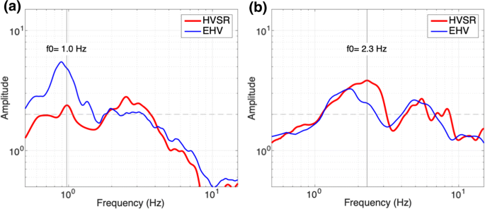

  

  Horizontal-to-Vertical spectral ratios calculated from earthquake recordings (EHV, in blue) and seismic noise (HVSR, in red) for stations (a) SP-KSP17 (Spoleto) and (b) IV-GUMA (Gualdo di Macerata). The vertical line indicates the value of the fundamental resonance frequency f0. The dashed horizontal line indicates the amplitude value of 2

• (b) Amplification factors of the peak ground motion The outcomes of the residual analysis using the ITA10 as reference model were exploited to evaluate the amplification of peak ground acceleration (PGA) and velocity (PGV). The peak amplification factors (FPGA and FPGV for the peak acceleration and velocity, respectively) were evaluated considering the residuals and estimated as the logarithmic difference between observations and predictions for the EC8-A site category. The total residuals were decomposed into between-event (median residual of single earthquakes) and within-event (median residuals, after correction of the single record by the between-event term) components (Al Atik et al. 2010; Lanzano et al. 2017). The within-event residuals were used to calculate the site-to-site term, $\delta$S2S_s, and its associated variability, $\phi_{0,s}$ for each station (Rodriguez-Marek et al. 2011; Luzi et al. 2014). These terms quantify the systematic amplification/deamplification of the observed ground motion at a given station with respect to the GMPE predictions.

• (c) Identification of the reference sites Empirical techniques to evaluate spectral amplifications make use of reference sites, i.e., stations installed on outcropping rock with a flat site response. The identification of such sites is implicit in the scope of this study. The WGs defined some common criteria for selection of the reference sites in accordance with the main indications provided in the literature (Steidl et al. 1996; Felicetta et al. 2018), which were applied to the collected dataset. Since the site classifications of several stations were missing, the soil conditions were disregarded, and priority was given to the seismological proxies. Following Luzi et al. (2018, this issue), the site-to-site terms were estimated with respect to the predictions for rock sites to identify stations with a site response similar to the EC8-A class of the ITA10 model.

  These proxies are as follows: (1) flat HVSR or EHV, i.e., amplitude values uniformly less than 2 within the analysed frequency range; (2) $\delta$S2S_s around zero for PGA, PGV and 3 spectral ordinates (at periods T = 0.1 s, 0.3 s, 1.0 s), i.e., included in the range [− 0.2–0.2] s and $\phi$_0,s lower than the ITA10 within-event standard deviation; and (3) a distance between the reference and investigated site of less than 5 km in the Standard Spectral Ratio analysis. The values of $\delta$S2S_s and $\phi$_0,s for the investigated ground motion parameters of the stations that meet criterion (2) are listed in Table 1 and plotted in Fig. 1 of the Electronic Supplement.

  Among the stations satisfying the three conditions, we selected the 6 sites listed in Table 3 (OX.CP06, OX.MN06, IT.LSS, IT.SLO, IV.T1217, IT1221) for the Phase 2 analyses; the corresponding values of $\delta$S2S_s and $\phi$_0,s are shown in Fig. 7. For the sake of completeness, Table 3 also includes the reference sites relative to the Norcia and Spoleto networks that were selected based on the surface geology and the trends of the EHV and HVSR curves, as well as those used in Phase 1. The locations of the stations in Table 3 are shown in Fig. 4 (red triangles in the right panel).

  Fig. 7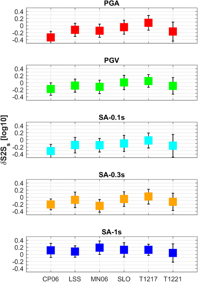

  

  $\delta$ S2S ± $\phi$_0,s for the 6 reference stations in the Central Italy dataset used in Phase 2 by the INGV-MI + UNIGE working group and reported in Table 3

• (d) Spectral amplification functions Two reference site methods, the standard spectral ratio (SSR) (Borcherdt 1970; Field and Jacob 1995) and the generalized inversion technique (GIT) (Andrews 1986; Castro et al. 1990) are usually adopted to evaluate the empirical amplification factors of the recording stations. In the SSR method, the spectral ratio between the same components of the ground motion recorded at two nearby stations (i.e., few kilometres of distance) is considered to validate the assumption that the reference site contains the same source and propagation contribution as the estimated site. Under such conditions, the spectral ratio of the two recordings provides a direct assessment of the site amplification relative to the reference. In contrast to the SSR method, the GIT method exploits large datasets composed of multiple stations and events to separate the site contributions from those relative to the source and propagation path. It consists of building a linear system of equations by expressing the FAS as follows:

  $$\log_{10} FAS_{es} = \log_{10} S_{e} + \log_{10} A_{es} + \log_{10} G_{s}$$

  (1)

  where S is the source spectra of the earthquake e, G is the amplification at site s, and A_es is the attenuation along the source-to-station path. The system of Eq. (1) can be solved using a parametric approach, where the unknown functions related to the source and propagation are expressed in terms of standard models (e.g., Kawase 2006; Drouet et al. 2011), or following a non-parametric inversion scheme (e.g., Castro et al. 1990; Oth et al. 2008; Pacor et al. 2016), where the source and propagation are part of the unknown of the problem.The methods used in this study to calculate the spectral amplification functions are well consolidated and implemented into robust and verified procedures. The parametric approach was adopted by the OGS to evaluate the site response at the stations installed in the Arquata-Montegallo area during Phase 1 (Laurenzano et al. 2018) and in the Spoleto municipality during the microzonation study performed in 2005–2006. The results of the latter study were included in Phase 2. In these cases, GITANES software was used (Klin et al. 2018) and the spectral amplification function was obtained from the Fourier amplitude spectra (GIT_FAS). This code considers the source and the seismic response terms as the unknowns of the problem, and the propagation term is estimated based on the pre-defined propagation model and the known location of the seismic sources (Laurenzano et al. 2018).The non-parametric scheme was followed to estimate the site functions of the Amatrice-Accumoli area during Phase 1 and for most of the Phase 2 stations. In this approach, no functional forms are pre-imposed to the source spectra and path terms; instead, they are considered unknowns of the problem similar to the site response terms and are solved simultaneously. Following Pacor et al. (2016), the inversion was performed in a single step (Oth et al. 2011) for the horizontal (geometric mean) and vertical components. Since we are interested in the site contribution, the hypocentral distances ranged from 15 to 125 km to exclude data that may be affected by source effects. The system was solved in a least-squares sense (Paige and Saunders 1982) and 100 bootstrap replications were performed at each frequency to evaluate the uncertainties (Efron 1979). In this study, the system of Eq. (1) was built for both the Fourier spectra and acceleration response spectra (SA). Although the SA does not depend linearly on the input motion, Bindi et al. (2017) showed that the amplification functions obtained for SA (GIT_SA) are comparable to those obtained for FAS, only differing in the high frequency range and overall amplification levels. The advantage of providing the spectral amplification in terms of SA instead of FAS is that they can be used directly to multiply the reference spectrum on rock to obtain the corresponding site-specific response spectrum. To solve Eq. (1), both the parametric and non-parametric approaches must fix the reference stations, constraining their amplification function to one; the selected stations for the study cases in this work are listed in Table 3. As an example, Fig. 8 shows the horizontal and vertical amplification functions for the same sites as in Fig. 6. For Spoleto, the empirical site functions are inferred from the parametric inversion of the FAS; for Gualdo di Macerata, the non-parametric inversion of SA is used. These cases show a behaviour observed in several other cases, e.g., the vertical component features relevant amplification with a higher resonant frequency. As a consequence, the use of the EHV as a proxy of the expected amplification at the sites may be misleading. Notably, the amplification functions were calculated by only one working group for each site, except for the case discussed in Sect. 5; therefore, no cross-validation between the parametric and non-parametric approaches can be done.

  Fig. 8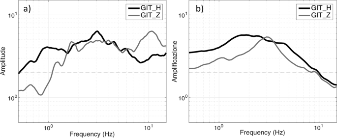

  

  Spectral amplification curves obtained by the GIT for (a) station SP-KSP17 (Spoleto) from the Fourier amplitude spectra (FAS) using a parametric approach, and (b) for station IV-GUMA (Gualdo di Macerata) from the acceleration response spectra (SA) using a non-parametric approach. The black and grey curves correspond to the horizontal and vertical components, respectively. The dashed horizontal line indicates the amplitude value of 2

• (e) Site-specific Response Spectra As established by the CMS and formalized by the Extraordinary Commissioner for the reconstruction (Ordinance n. 55, 2018), the response spectra (RS) are estimated by applying the spectral amplification functions (previous point d) to a seismic input compatible with the Uniform Hazard Spectrum (UHS), calculated for a 10% exceedance probability level in 50 years (return period 475 y), as defined by the Italian seismic code (NTC08). The seismic input was provided for each MS3-locality of Phase 2 by the Seismic Input Thematic Unit (UTIS) operating within the project (Luzi et al. 2019). According to the prescriptions, it is composed of a set of 7 spectrum-compatible accelerograms from [0.1–1.1] s. Although this approach cannot be assimilated rigorously to a probabilistic hazard method because it produces ground-motion levels whose exceedance rates are not exactly known, it is the simplest way to introduce the site effects (Barani and Spallarossa 2017) and it meets the requirements of the Italian Guidelines for Seismic Microzonation. A more detailed discussion of this topic is beyond the scope of this paper. For the RS, different computation methods were followed that correspond to the two approaches adopted. For the GIT computed from the Fourier spectra, the site-specific response spectrum (RS_FAS) was estimated by multiplying the GIT_FAS spectral amplification function with the Fourier amplitude spectrum of the seismic input, maintaining the input signal phase. For the GIT computed from the response spectra, the site-specific response spectrum (RS_SA) was estimated as a simple product of the seismic input and the GIT_SA at corresponding periods.

  Figure 9 shows an example of the results obtained for the localities of Spoleto and Gualdo di Macerata. The RS were calculated using the GIT curves (horizontal component) shown in Fig. 8 for the two sites. Note that the figures in the forms only report the median value estimated for the RS.

  Fig. 9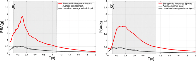

  

  Red line: Site-specific Response Spectra (median value, horizontal component) obtained for stations (a) SP-KSP17 (Spoleto) and (b) IV-GUMA (Gualdo di Macerata). Thin black line: average seismic input corresponding to the spectral acceleration with a 10% exceedance probability level in 50 years (return period of 475 years). Grey line: linearized reference seismic input (as defined by the SM Working Group 2015). Grey shaded area: spectral compatibility band [0.1–1.1] s

• (f) Amplification factors This class of parameters includes the following: (1) spectral amplification factors (FAj, j = 1, 2, 3), which are computed from the Site-specific Response Spectra (point e) for three period bands and (2) peak amplification factors, which are computed for Peak Ground Velocity (PGV) and Peak Ground Acceleration (PGA), as described in point b). The FAj is calculated according to the Italian Guidelines for Seismic Microzonation (SM Working Group, 2015) as the ratio between the average values of the output and input response spectra over the j-th period band, according to the following formulas:

  $$FAj = \frac{{SA_{j}^{out} }}{{SA_{j}^{in} }}\quad {\text{for}}\;j = 1,2,3$$

  (2)

  where $\left\langle \cdot \right\rangle$ represents the geometric average,

  $$SA_{j}^{k} = \frac{1}{{\Delta T_{j} }}\mathop \smallint \limits_{{\Delta T_{j} }}^{ } RS^{k} \left( T \right)dT\quad with\;k = out,in,$$

  (3)

  and RS^k(T) is the elastic acceleration response spectrum equal to RSⁱⁿ(T) for the input and RS^out(T) for the output. The FAs were computed for the following three period intervals: ΔT1 [0.1–0.5] s; ΔT2 [0.4–0.8] s; ΔT3 [0.7–1.1] s that cover the entire period of interest for the buildings in the areas affected by the 2016–2017 seismic sequence (except for very large buildings such as dams and viaducts, for which specific studies are prescribed). The 3 amplification factors FA1, FA2, and FA3 were named accordingly. For each FA, the geometric average and uncertainty (first standard deviation) were computed and reported. As an example, Fig. 10 shows the amplification factors and related uncertainty obtained for the localities of Spoleto and Gualdo di Macerata. The FA and FPGV or FPGA are indicated by coloured squares and circle symbols, respectively.

  Fig. 10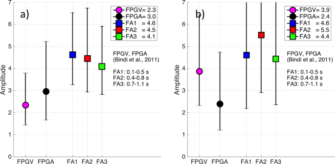

  

  Amplification factors calculated for stations (a) SP-KSP17 (Spoleto) and (b) IV-GUMA (Gualdo di Macerata). FPGV and FPGA (coloured circles): amplification factors of PGV and PGA with respect to those predicted by the ground motion prediction equation of Bindi et al. (2011). FA1, FA2, FA3: average spectral amplification factors (coloured squares) in the period intervals of [0.1–0.5] s, [0.4–0.8] s, and [0.7–1.1] s, respectively. The associated uncertainties (first standard deviation) are also displayed. The average values are listed in the legend

5 Validation tests

As described in Sects. 3 and 4, the UTAS activity was carried out by several WGs, which used different data and methodologies and independently analysed different groups of stations to obtain the products. Although all the methods adopted for the site response calculation are well consolidated in seismological practice and were implemented in robust and verified procedures (see Sect. 4), we verified that the results obtained by different methods were consistent with each other at a single site.

The test site used for this purpose is located at the Spoleto (Fig. 2) municipal building, within the historical center of the town. This site is unique for the aim of this study for two important reasons. First, it has hosted two different stations at different times that were located approximately at the same site, namely, the permanent station of the Italian Strong Motion Network (RAN) IT-SPO1, managed by the DPC, and the temporary station SP-KPS03, which was installed by the OGS as part of a MS3-study committed by the Spoleto Municipality. Being that area of Spoleto characterized by Plio-Pleistocene continental deposits made by consolidated clay and compacted gravel with different degrees of cementation lying on stiff carbonatic rock of marine origin and urbanized by stately buildings since centuries, the soil features a stable geo-mechanical behaviour (Vuan et al. 2007; Sotera and Arcaleni 2018). Second, the datasets of the two stations were independently analysed by two different WGs. Thus, a direct comparison of the results obtained by the two WGs for this station allows for us to verify the consistency of the two adopted approaches and the stability and reliability of the estimations using different recording datasets. Table 4 summarizes the main features of the two stations, the installed instrumentation, number of events, reference site and methodologies used for site response evaluation.

Table 4 Main features of the two stations located in the Spoleto municipal building analysed in the validation test

For the IT-SPO1 station, the INGV-MI + UNIGE WG used the GIT_SA method considering the reference site composed of the 4 stations listed in Table 3; for the SP-KSP03 station, the OGS WG used the GIT_FAS method considering the reference site SP-KSP01 (Table 3). The elastic response spectra were evaluated accordingly (i.e., RS_SA and RS_FAS). Note that the two cases differ in the acquisition period and thus in the datasets and number of selected events (acquisition period 2015–2017 and 113 events for IT-SPO1; acquisition period 2005–2006 and 27 events for SP-KSP03). The graphs of Fig. 11 compare the results obtained for the two stations—note that the amplification is estimated using SA for IT-SPO1 and FAS for SP-KSP03—and show good similarity in general features such as the shape, amplitude, resonant frequency and higher peaks. The amplification factors are comparable, with values of one included in the standard deviation of the other. Although limited to a single case, this validation confirms the robustness and reliability of the adopted approach.

Fig. 11

Comparison of the results obtained for the IT-SPO1 and SP-KSP03 stations installed at the offices of the municipality of Spoleto. The thick and thin lines represent the estimates obtained for the IT-SPO1 (based on SA) and SP-KSP03 (based on FAS) stations, respectively. The panels show the following: GIT calculated for the (a) horizontal and (b) vertical components; (c) EHV ratio; (d) site-specific response spectra; and (e) amplification factors FAs, FPGV and FPGA

6 Deliverables and results

The results of this study were summarized for each site into a site-specific form delivered to the CMS. These forms are useful for the MS3 of the damaged municipalities and their reconstruction. For sites where multiple estimates were obtained by different WGs or using different procedures, the consistency of the results was verified, and one value/curve was provided. GIT_SA was chosen over GIT_FAS since the former allows for more direct computation of the RS by multiplying by the reference seismic input. Moreover, GIT analysis was preferred over SSR since GIT is considered a more robust technique that allows for the use of a larger number of recordings. GIT also has some limitations. In the case where the maximum interstation distance is small with respect to the hypocentral distances, the ray paths between a source and all the stations are nearly coincident. In such conditions of short and similar ray paths, GIT could fail to separate the effects of site, source, and attenuation (Parolai et al. 2000; Ameri et al. 2011). Furthermore, GIT may use several reference sites—a sort of average, virtual rock site—usually located far from the investigated sites and with properties that can be very different from those of a true reference site located near the investigated site. In this case, the estimated amplification may differ from that calculated by SSR using a local reference site and may not reflect some specificities of the investigated site.

Figure 12 shows an example of the form produced for station IV-RM18 located at Fano Adriano (Fig. 2). Each form is composed of four sections. The first is a header that reports a summary of useful information on the position and instrumentation of the recording station, the site seismic response and seismological data analysis. The second section displays three maps that are useful for locating the site station at regional and local scales and with respect to the geolithology. The third and fourth sections represent products a-d (see Sect. 4) from the site response analysis. The third section shows the amplification computed by GIT for the horizontal and vertical components and the H/V spectral ratios computed from noise and earthquake recordings. The last section displays the site-specific acceleration response spectrum and amplification factors. The collection of the forms produced for all sites can be found at the following: https://annuminas.igag.cnr.it/share.cgi?ssid=0aW4WM0.

Fig. 12

Station form produced for the IV-RM18 station at the Fano Adriano site. It is composed of four sections (see the text). The header reports information on the site location, instrumentation, recording data, the site’s fundamental frequency, if any, the reference site used, number of total recordings, and WG. The three maps allow for locating the site station at regional and local scales through a road map (taken from Open Street Map) and with respect to the geolithology (taken from the Geoportale Nazionale http://www.pcn.minambiente.it/mattm/). The last two sections contain four figures that represent (from top to bottom and left to right) the spectral amplification for the horizontal and vertical components, the H/V spectral ratios computed from noise and earthquakes, the site-specific acceleration response spectrum, and the scalar amplification factors, respectively. The labels within the panels are in Italian since the form was delivered to the Italian authorities

Considering the scope of our study and the extent of the investigated area, we cannot discuss the results obtained for each site in detail. However, we summarize some significant outcomes of the two phases to provide some examples of the results. Figure 13 shows the FA1 from Phase 1. There is notable variability in the amplification values, which is also due to the heterogeneity of the measurement locations. In general, most FA1 do not exceed 3. Six sites feature FA1 amplification larger than 4, namely, Pescara del Tronto and Castro in the Arquata-Montegallo area, located on Quaternary deposits overlying bedrock (Laurenzano et al. 2018), and sites MZ15-MZ17-MZ24 (located on gravel and sands of Quaternary deposits) and MZ104 in the Amatrice-Accumoli area.

Fig. 13

Spectral amplification factor FA1 (period band [0.1–0.5] s) estimated for the Phase 1 localities. (a) Map of the investigated area. Coloured symbols represent the FA1 value (see legend). Squares and circles indicate the sites in the Arquata-Montegallo and Amatrice-Accumoli areas, respectively. (b) Detail for the Amatrice municipality corresponding to the black rectangle in panel (a)

Figure 14 shows statistics on the amplification factors and resonant frequency for both phases. The empirical distributions of the amplification factors are mainly unimodal for both phases. The FAs distributions feature a sharper bell shape—note that the value intervals are defined according to a log-scale distribution—for Phase 1 than for Phase 2. Phase 1 features varying behaviour between the short-period amplification (FA1) and the medium- and long-period amplifications (FA2 and FA3, respectively), i.e., weak amplifications (i.e., values in the range 1–1.4) occur much more frequently in the medium- and long-period bands (approximately 15% of the total sites) than in the short-period band (approximately 5%); this trend inverts for larger amplification values. FA1 sets the maximum distribution value (30%) for moderate amplification (range 1.4–2) and then decreases progressively as the amplification value increases. FA2 and FA3 feature opposite behaviour, i.e., they increase progressively with the amplification and reach their maximum (approximately 25%) with the strong amplification classes (range 2–2.8 and 2.8–4, respectively). For all FAs, approximately 5–10% sites feature very strong or extreme amplification (classes 4–5.6 and 5.6–8, respectively). The peak amplification factors feature analogous behaviour if one assimilates PGA and PGV to FA1 and FA2-FA3, respectively; for nearly 50% of the sites, PGA is weakly amplified, and this decreases progressively as the PGA amplification increases. The FPGV distribution shows a bell shape with maximum (approximately 40%) at moderate amplification (class 1.4–2). The resonant frequencies f₀ are mostly distributed among the three classes that span the frequency range of engineering interest for the residential/common buildings (1–8 Hz). Approximately 25% of the sites feature no resonance and none show broad-band resonance.

Fig. 14

Statistical distribution of the amplification factor values and resonant frequencies estimated for the sites analysed in Phases 1 (upper row of panels) and 2 (lower row). The panels show the three spectral amplification factors (a and d); the PGV and PGA amplification factors (b and e); and the resonant frequency (c and f). Columns NR and BB in panels (c) and (f) indicate a “non-resonant site” (i.e., flat HVSR) and “broad-band” HVSR, respectively. The classes of values y₁ − y₂ are defined as y₁ < y ≤ y₂. Note that the bins of both the amplification factors and the resonant frequency are defined according to a geometric progression

Phase 2 features rather similar distributions for both the spectral and peak amplifications. Approximately 10% of the sites feature neutral behaviour or deamplification for the FAs (approximately 10–15% for PGA and PGV). The distributions feature a wide range of well-populated classes, with amplification values between 1 and 4 more or less homogeneously represented by approximately 15–25% of the total sites; in this range of values, note that FA1 is slowly increasing, with maximum of 30% at 2.8–4, whereas FA3 is slowly decreasing, with maximum at 1–1.4, and FA2 remains nearly constant, represented by nearly 20% in each class. The distribution of the peak amplification is mostly represented by the class of moderate amplification (approximately 25% of the sites with FPGA-FPGV 1.4–2), and it features a light dominance of FPGA at low amplification levels (≤ 1.4) and FPGV at higher values. The resonant frequencies are mostly distributed among the four classes that span from 0.5 to 8 Hz. 20% and approximately 5% of the sites feature no resonance or broad-band resonance, respectively.

As an additional example of the importance of our study, we evaluated if there is general agreement between the amplification estimated by the analysis proposed in this paper and that assessed within the MS3 study. We selected the study cases of Capitignano and Montereale, two hamlets located next to each other in an area of approximately 2 km² (Fig. 2). Each of these localities hosted at least 3 recording sites analysed in this work. We focused on the comparison of spectral amplification factors calculated in the three period bands specified above.

In the SM, the amplification is assessed by 1D or 2D numerical methods simulating the physical response of the site (SM Working Group 2015). The numerical simulations use local models based on detailed engineering and geological knowledge and use the seismic input compatible with the UHS as the loading signal (Luzi et al. 2019; Pergalani et al. 2019). The seismic amplification is expressed in terms of numerical FAs calculated the same as the experimental values described in Sect. 4. Notably, the Italian microzoning approach (SM Working Group 2015) classifies the following: (1) stable zones, for which the FA is assumed to be 1 (e.g., outcropping of seismic bedrock); (2) stable zones prone to local amplification, for which the FAs are assessed numerically; and (3) unstable zones, where the hazard related to seismically induced phenomena such as liquefaction or surface faulting is evaluated (also including seismic amplification).

The Capitignano urbanized area lies within the Montereale sedimentary basin (Chiarini et al. 2014) at the foothills of the relief that borders the basin to the NW (Fig. 15a). This sector of the basin is filled with quaternary lacustrine deposits and debris, colluvial and alluvial fan deposits widely outcrop in the piedmont area. The relief is made of Flysch (Fig. 15a), which represents the local bedrock and is characterized by the presence of the active Capitignano fault (Boncio et al. 2004; Galadini and Messina 2004; Civico et al. 2016). As result of the tectonic processes, the bedrock is locally highly jointed and weathered. In this area, three seismic stations of the XO network were deployed, namely, CP02, CP04 and CP05 (please refer to the supporting material for the station monographies).

Fig. 15

(a) Geological map of the Capitignano area with seismic station locations; the SM study was performed in the perimeter depicted in light grey (modified from Nocentini 2018). (b) SM map of Capitignano with seismic station locations; the blue colour distinguishes the stable zone with respect to the zones prone to seismic amplification (other colours in the panel), for which the FAs have been calculated numerically (modified from Nocentini 2018). (c) Numerical vs experimental FAs (average value); symbols represent stations and colours represent the spectral amplification factors calculated in the three period bands (FA1 [0.1–0.5] s; FA2 [0.4–0.8] s; FA3 [0.7–1.1] s)

According to the final SM study (Nocentini 2018), the CP02 station was located on the quaternary filling of the basin (SM, yellow; Fig. 15a), and CP04 and CP05 were located on Flysch (SFLPS, pale blue) and alluvial fan deposits (GM, green), respectively. Moreover, Fig. 15b shows that sites CP02 and CP05 are located in areas prone to seismic amplification and CP04 is located inside the zone classified as stable (seismic bedrock outcropping, blue area in Fig. 15b).

In the following, we compare the numerical FA values computed in the framework of the SM study (Nocentini 2018) with the experimental values estimated from the recorded data. The numerical FAs for site CP04 were assumed to be equal to 1 in agreement with the SM regulation for zones classified as stable. The experimentally derived FAs for CP04 are slightly larger than the numerical ones (approximately 1.1–1.2 for FA2 and FA3), with the largest value (approximately 1.6) for FA1 (Fig. 15c). This larger value of amplification at the short-period band is likely related to the local weathered and jointed condition of the outcropping bedrock, which results in a reduction of the rock stiffness at shallow depths. For CP05, the experimental FAs are slightly larger than the numerical ones and are almost equal for the short-period band FA1 (Fig. 15c). Their values are in agreement with the geological model, as a relevant amplification can be expected for the prevalent loose gravel deposits overlying Flysch bedrock (Fig. 15a). For CP02, the numerical FAs underestimate the experimentally obtained values, although they show the similar trend of increasing FA with increasing period (Fig. 15c).

The urbanized area of Montereale lies mostly on the relief, which is a monocline made by Flysch bedrock (ALS, blue; Fig. 16a). Around the relief, to the S and E, lacustrine deposits (MH, brown) widely crop out and the Flysch is partly covered by colluvial deposits (SM-SW, yellow) SW of the urbanized area. Geophysical surveys showed that this basin-filling material may have thickness greater than 100 m (Chiarini et al. 2014). The distinction in the two different geological conditions, i.e., outcropping bedrock vs basin infilling, is apparent in the final SM map (Fig. 16b) and in the seismological data recorded in the two sectors.

Fig. 16

(a) Geological map of the Montereale area with seismic station locations; the SM study was performed in the perimeter depicted in light grey (modified from Agnelli et al. 2018). (b) SM map of Montereale with seismic station locations; the different colours distinguish the unstable zones (yellow) with respect to the seismic amplification prone zones (other colours in the panel); the numerically derived FAs for the three different period bands were calculated for both zone types (modified from Agnelli et al. 2018). (c) Numerical FAs vs experimental FAs (average value); symbols represent stations and colours represent the spectral amplification factors calculated in the three period bands (FA1 [0.1–0.5] s; FA2 [0.4–0.8] s; FA3 [0.7–1.1] s)

In this area, three seismic stations of the XO network were deployed, namely, MN08, MN06 and MN03 (please refer to the supporting material for the station monographies). The SM study (Agnelli et al. 2018) distinguishes an unstable zone prone to seismically induced liquefaction (yellow area in Fig. 16b), where MN03 is located, and some zones prone to seismic amplification (other coloured areas in Fig. 16b), including those where the underlying bedrock outcrops as weathered Flysch, where MN06 and MN08 are located.

For the MN06 and MN08 stations located on Flysch, the experimental FAs are generally close to 1 and the numerical FAs slightly overestimate them, with the exception of FA1 for MN06, which has experimental value smaller than 1 (Fig. 16c). The experimental FAs at station MN03, deployed on lacustrine sediments at the base of the Montereale relief, are larger than 2 in all period bands (with a maximum of approximately 3.5 in the [0.4–0.8] s band; Fig. 16c). The numerically derived FAs for the lacustrine deposits feature some severe discrepancies with respect to those derived from observations, especially for longer periods. This may be due to several causes such as inconsistencies in the subsurface model in the assessment of the depth of the seismic bedrock, which can be at more than 100 m, or the occurrence of basin-edge effects that were not predicted by the numerical models.

For the described examples, the general geological model reconstruction is in agreement with the seismological analyses. The geological models and SM studies provide key elements to interpret the observed amplification levels. For bedrock outcroppings, we observed fairly good agreement between the numerically and experimentally obtained FAs. The agreement is significant considering that the numeric FAs were retrieved for a subsurface model representative of a relatively wide area whereas the experimental estimates are inherently site-specific. However, for these case-studies, there were non-negligible discrepancies for the FAs estimated for areas where soft sediments crop out. This may be related to limitations in the approach used for SM, as 1D and 2D numerical models may be inadequate to reproduce complex geological conditions. Therefore, we suggest extending this comparison to other areas investigated in the SM of Central Italy to better understand the advantages and limitations of the SM approach.

7 Conclusions

We described the seismological analyses performed for the seismic microzonation study for reconstruction of the 138 municipalities damaged by the 2016–2017 seismic sequence in Central Italy. This study was carried out in two phases, the emergency Phase 1, including the deployment of temporary seismic networks within the epicentral area, and the post-emergency Phase 2, including the analyses of the available digital seismological data for the damaged municipalities. Significant efforts were made to provide homogeneous and comparable results to the CMS and National Authorities for the reconstruction of the damaged towns.

Phase 1 concerned the 4 municipalities of Amatrice, Accumoli, Arquata del Tronto, and Montegallo. Since this phase is presented in other specific articles, we summarized the main features and results.

The approach adopted for Phase 2 represents the most innovative part of our study. We described the procedure adopted for selecting the stations used for evaluating the site response of the MS3-localities identified by the Italian authorities using earthquake and noise recordings. Then, we defined the set of key products to be determined. A huge amount of data recorded over the course of several years at approximately 180 instrumented sites was analysed by different working groups operating simultaneously. The results were collected and homogeneously summarized in site-specific forms that were delivered to the CMS, providing several important indications to be used for the MS3 of the damaged municipalities and their reconstruction. The whole activity was performed in the very short period of 2–3 months. Our study shows that different expert groups can successfully work simultaneously, provided that standard processing procedures and scientific products are clearly defined.

Despite the different purposes of the seismic networks, the results of our study show that the urbanized territory in Central Italy is generally prone to seismic amplification. Reference sites were only a small subset of the analysed stations. Therefore, care should be taken when comparing standard seismic hazard estimates against observed values, as the latter often are recorded by stations for which local site effects cannot be ruled out (e.g., Barani et al. 2017). Hence, characterization of the recording sites remains a fundamental issue.

Although the approach presented in this paper can be improved—for instance, a more rigorous link of the RS to a uniform hazard concept or description of the uncertainty—this strategy can be taken as a reference approach for planning an extensive analysis of the huge seismological dataset for the Italian territory and for optimal future seismological interventions in post-earthquake phases.

Appendix

This Appendix reports the stations that were analysed during Phases 1 and 2 of this study.

Table 5 Temporary stations installed in the municipalities of Arquata del Tronto and Montegallo that were analysed during Phase 1

Table 6 Temporary stations installed in the municipalities of Amatrice and Accumoli that were analysed during Phase 1

Table 7 Temporary and permanent stations installed in the 134 municipalities that were analysed during Phase 2

References

Agnelli A, Di Lizia E, Totani F, Germani G (2018) Comune di Montereale (AQ) “Studio di Microzonazione sismica di livello 3 del Comune di Montereale, ai sensi dell’Ordinanza del Commissario Straordinario del Governo n° 24 registrata il 15/05/2017 al n°1065” (in Italian)
Al Atik L, Abrahamson N, Bommer J, Scherbaum F, Cotton F, Kuehn N (2010) The variability of ground-motion prediction models and its components. Seismol Res Lett 81(5):794–801. https://doi.org/10.1785/gssrl.81.5.794
Ameri G, Oth A, Pilz M, Bindi D, Parolai S, Luzi L, Mucciarelli M, Cultrera G (2011) Separation of source and site effects by generalized inversion technique using the aftershock recordings of the 2009 L’Aquila earthquake. Bull Earthq Eng 9(3):717–739
Andrews DJ (1986) Objective determination of source parameters and similarity of earthquakes of different size. Earthq Source Mech 37:259–268
Barani S, Spallarossa D (2017) Soil amplification in probabilistic ground motion hazard analysis. Bull Earthq Eng 15(6):2525–2545
Barani S, Albarello D, Spallarossa D, Massa M (2017) Empirical scoring of ground motion prediction equations for probabilistic seismic hazard analysis in Italy including site effects. Bull Earthq Eng 15(6):2547–2570
Bard PY, SESAME-team (2005) Report D23.12—Guidelines for the implementation of the H/V spectra ratio technique on ambient vibration measurements, processing and interpretation—Technical report. European Commission—Research Generale Directorate Project N° EVG1-CT-2000-00026 SESAME, 2005. http://sesamefp5.obs.ujfgrenoble.fr
Bindi D, Pacor F, Puglia R, Massa M, Ameri G, Paolucci R (2011) Ground motion prediction equations derived from the Italian strong motion data. Bull Earthq Eng 9(6):1899–1920. https://doi.org/10.1007/s10518-011-9313-z
Bindi D, Spallarossa D, Pacor F (2017) Between-event and between-station variability observed in the Fourier and response spectra domains: comparison with seismological models. Geophys J Int 210(2):1092–1104. https://doi.org/10.1093/gji/ggx217
Boncio P, Lavecchia G, Pace B (2004) Defining a model of 3D seismogenic sources for Seismic Hazard Assessment applications: the case of central Apennines (Italy). J Seismolog 8(3):407–425
Bonini L, Maesano FE, Basili R, Burrato P, Carafa MMC, Fracassi U, Kastelic V, Tarabusi G, Tiberti MM, Vannoli P, Valensise G (2016) Imaging the tectonic framework of the 24 August 2016, Amatrice (Central Italy) earthquake sequence: new roles for old players? Ann Geophys 59(Fast Track 5). https://doi.org/10.4401/ag-7229
Bonnefoy-Claudet S, Cotton F, Bard PY (2006) The nature of noise wavefield and its applications for site effects studies. A literature review. Earth Sci Rev 79:205–227
Borcherdt RD (1970) Effects of local geology on ground motion near San Francisco Bay. Bull Seismol Soc Am 60:29–61
Cara F, Cultrera G, Riccio G, Amoroso S, Bordoni P, Bucci A, D’Alema E, D’Amico M, Cantore L, Carannante S, Cogliano R, Di Giulio G, Di Naccio D, Famiani D, Felicetta C, Fodarella A, Franceschina G, Lanzano G, Lovati S, Luzi L, Mascandola C, Massa M, Mercuri A, Milana G, Pacor F, Piccarreda D, Pischiutta M, Pucillo S, Puglia R, Vassallo M, Boniolo G, Caielli G, Corsi A, de Franco R, Tento A, Bongiovanni G, Hailemikael S, Martini M, Paciello A, Peloso A, Verrubbi V, Gallipoli MR, Tony Stabile TA, Mancini M (2019) Temporary dense seismic network during the 2016 Central Italy seismic emergency for microzonation studies, submitted to Nature Scientific Data
Castro RR, Anderson JG, Singh SK (1990) Site response, attenuation and source spectra of S waves along the Guerrero, Mexico, subduction zone. Bull Seismol Soc Am 80:1481–1503
Cavinato GP, De Celles PG (1999) Extensional basins in the tectonically bimodal central apennines fold-thrust belt, Italy: response to corner flow above a subducting slab in retrograde motion. Geology 27:955–958
Chiaraluce L, Di Stefano R, Tinti E, Scognamiglio L, Michele M, Casarotti E, Cattaneo M, De Gori P, Chiarabba C, Monachesi G, Lombardi A, Valoroso L, Latorre D, Marzorati S (2017) The 2016 Central Italy seismic sequence: a first look at the mainshocks, aftershocks, and source models. Seismol Res Lett 88(3):757–771. https://doi.org/10.1785/0220160221
Chiarini E, La Posta E, Cifelli F, D’Ambrogi C, Eulilli V, Ferri F, Marino M, Mattei M, Puzzilli LM (2014) A multidisciplinary approach to the study of the Montereale Basin (Central Apennines, Italy). Rendiconti Lincei 25(2):177–188. https://doi.org/10.1007/s12210-014-0311-3
Civico R, Blumetti AM, Chiarini E, Cinti FR, La Posta E, Papasodaro F, Sapia V, Baldo M, Lollino G, Pantosti D (2016) Traces of the active Capitignano and San Giovanni faults (Abruzzi Apennines, Italy). J Maps 12:453–459. https://doi.org/10.1080/17445647.2016.1239229
Cultrera G, Mucciarelli M, Parolai S (2011) The L’Aquila earthquake—a view of site effects and building behavior from temporary networks. Bull Earthq Eng 9(3):691–695. https://doi.org/10.1007/s10518-011-9270-6
Cultrera G, D’Alema E, Amoroso S, Angioni B, Bordoni P, Cantore L, Cara F, Caserta A, Cogliano R, D’Amico M, Di Giulio G, Di Naccio D, Famiani D, Felicetta C, Fodarella A, Lovati S, Luzi L, Massa M, Mercuri A, Milana G, Pacor F, Pischiutta M, Pucillo S, Puglia R, Riccio G, Tarabusi G, Vassallo M, Mascandola C (2016) Site effect studies following the 2016 Mw 6.0 Amatrice earthquake (Italy): the Emersito task force activities. Ann Geophys 59(Fast Track 5). https://doi.org/10.4401/ag-7189
D’Agostino N, Jackson JA, Dramis F, Funiciello R (2001) Interactions between mantle upwelling, drainage evolution and active normal faulting: an example from the central Apennines (Italy). Geophys J Int 147(2):475–497. https://doi.org/10.1046/j.1365-246X.2001.00539.x
Di Bona M (2016) A local magnitude scale for crustal earthquakes in Italy. Bull Seism Soc Am 106:242–258
Dolce M (2009) Mitigation of seismic risk in Italy following the 2002 S. Giuliano earthquake. Geotech Geol Earthq Eng 11:67–89
Dramis F (1992) Il ruolo dei sollevamenti tettonici a largo raggio nella genesi del rilievo appenninico. Studi Geologici Camerti, volume speciale 1992/l (1992), pp 9–16
Drouet S, Bouin MP, Cotton F (2011) New moment magnitude scale, evidence of stress drop magnitude scaling and stochastic ground motion model for the French West Indies. Geophys J Int 187:1625–1644
Efron B (1979) Bootstrap methods: another look at the Jackknife. Ann Stat 7(1):1–26
EMERGEO Working Group, Pucci S, De Martini P, Civico R, Nappi R, Ricci T, Villani F, Brunori C, Caciagli M, Sapia V, Cinti F, Moro M, Di Naccio D, Gori S, Falcucci E, Vallone R, Mazzarini F, Tarquini S, Del Carlo P, Kastelic V, Carafa M, De Ritis R, Gaudiosi G, Nave R, Alessio G, Burrato P, Smedile A, Alfonsi L, Vannoli P, Pignone M, Pinzi S, Fracassi U, Pizzimenti L, Mariucci M, Pagliuca N, Sciarra A, Carluccio R, Nicolosi I, Chiappini M, Dajello Caracciolo F, Pezzo G, Patera A, Azzaro R, Pantosti D, Montone P, Saroli M, Lo Sardo L, Lancia M (2016) Coseismic effects of the 2016 Amatrice seismic sequence: first geological results. Ann Geophys 59(Fast Track 5). https://doi.org/10.4401/ag-7195
Felicetta C, Lanzano G, D’Amico M, Puglia R, Luzi L, Pacor F (2018) Ground motion model for reference rock sites in Italy. Soil Dyn Earthq Eng 110:276–283. https://doi.org/10.1016/j.soildyn.2018.01.024
Ferrarini F, Lavecchia G, de Nardis R, Brozzetti F (2015) Fault geometry and active stress from earthquakes and field geology data analysis: the Colfiorito 1997 and L’Aquila 2009 Cases (Central Italy). Pure Appl Geophys 172(5):1079–1103. https://doi.org/10.1007/s00024-014-0931-7
Field EH, Jacob KHA (1995) Comparison and test of various site-response estimation techniques, including three that are not reference-site dependent. Bull Seism Soc Am 85(4):1127–1143
Galadini F, Messina P (2004) Early-middle Pleistocene eastward migration of the Abruzzi Apennine (central Italy) extensional domain. J Geodyn 37:57–81
Galli P, Galadini F, Pantosti D (2008) Twenty years of paleoseismology in Italy. Earth Sci Rev 88(1–2):89–117. https://doi.org/10.1016/j.earscirev.2008.01.001
Galvani A, Anzidei M, Devoti R, Esposito A, Pietrantonio G, Pisani AR, Riguzzi F, Serpelloni E (2012) The interseismic velocity field of the Central Apennine from a dense GPS network. Ann Geophys 55(5):1039–1049. https://doi.org/10.4401/ag-5634
Gruppo di Lavoro INGV sul terremoto in centro Italia (2016) Summary report on the October 30, 2016 earthquake in Central Italy Mw 6.5, https://doi.org/10.5281/zenodo.166238
ISIDe Working Group (2016) Version 1.0. https://doi.org/10.13127/iside
Kawase H (2006) Site effects derived from spectral inversion method for K-NET, Kik-net, and JMA strong-motion network with Special reference to soil nonlinearity in high PGA records. Bull Earthq Res Inst Univ Tokyo 81:309–315
Klin P, Laurenzano L, Priolo E (2018) GITANES: a MATLAB package for joint estimation of site spectral amplification and seismic source spectra with the generalized inversion technique. Seismol Res Lett 89(1):182–190. https://doi.org/10.1785/0220170080
Konno K, Ohmachi T (1998) Ground-motion characteristics estimated from spectral ratio between horizontal and vertical components of microtremor. Bull Seismol Soc Am 88(1):228–241
Lanzano G, D’Amico M, Felicetta C, Luzi L, Puglia R (2017) Update of the single-station sigma analysis for the Italian strong-motion stations. Bull Earthq Eng 15(6):2411–2428
Laurenzano G, Barnaba C, Romano MA, Priolo E, Bertoni M, Bragato PL, Comelli P, Dreossi I, Garbin M (2018) The Central Italy 2016–2017 seismic sequence: site response analysis based on seismological data in the Arquata del Tronto-Montegallo municipalities. Bull Earthq Eng. https://doi.org/10.1007/s10518-018-0355-3
Lavecchia G, Castaldo R, de Nardis R, De Novellis V, Ferrarini F, Pepe S, Brozzetti F, Solaro G, Cirillo D, Bonano M, Boncio P, Casu F, De Luca C, Lanari R, Manunta M, Manzo M, Pepe A, Zinno I, Tizzani P (2016) Ground deformation and source geometry of the 24 August 2016 Amatrice earthquake (Central Italy) investigated through analytical and numerical modeling of DInSAR measurements and structural-geological data. Geophys Res Lett 43(24):12389–12398. https://doi.org/10.1002/2016gl071723
Lermo J, Chávez-García F (1994) Are microtremors useful in site response evaluation? Bull Seismol Soc Am 84:1350–1364
Luzi L, Bindi D, Puglia R, Pacor F, Oth A (2014) Single-station sigma for Italian strong-motion stations. Bull Seismol Soc Am 104(1):467–483. https://doi.org/10.1785/0120130089
Luzi L, Pacor F, Lanzano G, Felicetta C, Puglia R, D’Amico M (2019) 2016–2017 Central Italy seismic sequence: strong-motion data analysis and design earthquake selection for seismic microzonation purposes. Bull Earthq Eng. Special Issue on “Seismic Microzonation of Central Italy” (submitted)
Luzi L, D’Amico M, Massa M, Puglia R (2018) Site effects observed in the Norcia intermountain basin (Central Italy) exploiting a 20-year monitoring. Bull Earthq Eng 17(1):97–118. https://doi.org/10.1007/s10518-018-0444-3
Marcellini A, Daminelli R, Tento A, Franceschina G, Pagani M (2001) The Umbria-Marche microzonation project: outline of the project and the example of Fabriano results. Ital Geotech J (Special Issue: The 1997–1998 Umbria-Marche Earthquake) 2:28–35
Margheriti L, Chiaraluce L, Voisin C, Cultrera G, Govoni A, Moretti M, Bordoni P, Luzi L, Azzara R, Valoroso L, di Stefano R, Mariscal A, Improta L, Pacor F, Milana G, Mucciarelli M, Parolai S, Amato A, Chiarabba C, de Gori P, Lucente FP, di Bona M, Pignone M, Cecere G, Criscuoli F, Delladio A, Lauciani V, Mazza S, di Giulio G, Cara F, Augliera P, Massa M, D’Alema E, Marzorati S, Sobiesiak M, Strollo A, Duval AM, Dominique P, Delouis B, Paul A, Husen S, Selvaggi G (2011) Rapid response seismic networks in Europe: lessons learnt from the L’Aquila earthquake emergency. Ann Geophys 54(4):392–399. https://doi.org/10.4401/ag-4953
Michele M, Di Stefano R, Chiaraluce L, Cattaneo M, De Gori P, Monachesi G, Latorre D, Marzorati S, Valoroso L, Ladina C, Chiarabba C, Lauciani V, Fares M (2016) The Amatrice 2016 seismic sequence: a preliminary look at the mainshock and aftershocks distribution. Ann Geophys 59(Fast Track 5). https://doi.org/10.4401/ag-7227
Milana G, Cultrera G, Bordoni P, Bucci A, Cara F, Cogliano R, Di Giulio G, Di Naccio D, Famiani D, Fodarella A, Mercuri A, Pischiutta M, Pucillo S, Riccio G, Vassallo M (2019) Local site effects estimation at Amatrice (Central Italy) through seismological methods. Bull Earthq Eng. https://doi.org/10.1007/s10518-019-00587-3
Moretti M, Abruzzese L, Abu Zeid N, Augliera P, Azzara RM, Barnaba C, Benedetti L, Bono A, Bordoni P, Boxberger T, Bucci A, Cacciaguerra S, Calò M, Cara F, Carannante S, Cardinale V, Castagnozzi A, Cattaneo M, Cavaliere A, Cecere G, Chiarabba C, Chiaraluce L, Ciaccio MG, Cogliano R, Colasanti G, Colasanti M, Cornou C, Courboulex F, Criscuoli F, Cultrera G, D’Alema E, D’Ambrosio C, Danesi S, de Gori P, Delladio A, De Luca G, Demartin M, di Giulio G, Dorbath C, Ercolani E, Faenza L, Falco L, Fiaschi A, Ficeli P, Fodarella A, Franceschi D, Franceschina G, Frapiccini M, Frogneux M, Giovani L, Govoni A, Improta L, Jacques E, Ladina C, Langlaude P, Lauciani V, Lolli B, Lovati S, Lucente FP, Luzi L, Mandiello A, Marcocci C, Margheriti L, Marzorati S, Massa M, Mazza S, Mercerat D, Milana G, Minichiello F, Molli G, Monachesi G, Morelli A, Moschillo R, Pacor F, Piccinini D, Piccolini U, Pignone M, Pintore S, Pondrelli S, Priolo E, Pucillo S, Quintiliani M, Riccio G, Romanelli M, Rovelli A, Salimbeni S, Sandri L, Selvaggi G, Serratore A, Silvestri M, Valoroso L, van der Woerd J, Vannucci G, Zaccarelli L (2012) Rapid response to the earthquake emergency of May 2012 in the Po Plain, Northern Italy. Ann Geophys 55(4):583–590. https://doi.org/10.4401/ag-6152
Moretti M, Pondrelli S, Margheriti L, Abruzzese L, Anselmi M, Arroucau P, Baccheschi P, Baptie B, Bonadio R, Bono A, Bucci A et al (2016) SISMIKO: emergency network deployment and data sharing for the 2016 central Italy seismic sequence. Ann Geophys 59(Fast Track 5). https://doi.org/10.4401/ag-7212
Mucciarelli M, Liberatore D (2014) Guest editorial: the Emilia 2012 earthquakes, Italy. Bull Earthq Eng 12(5):2111–2116. https://doi.org/10.1007/s10518-014-9629-6
Mucciarelli M, Cultrera G, Parolai S (2011) The L’Aquila earthquake—a view of site effects and structural behavior from temporary networks. Bull Earthq Eng 9(3):691–695
Nakamura Y (1989) A method for dynamic characteristics estimation of subsurface using microtremor on the ground surface. Q Rep RTRI 30:25–33
Nocentini M (2018) Comune di Capitignano (AQ) “Studio di Microzonazione sismica di livello 3 del Comune di Capitignano, ai sensi dell’Ordinanza del Commissario Straordinario n° 24 registrata il 15/05/2017 al n°1065” (in Italian)
Ori GG, Serafini G, Visentini G, Lucchi FR, Casnedi R, Colalongo ML, Mosna S (1993) Depositional history of the Pliocene-Pleistocene Adriatic foredeep (Central Italy) from surface and subsurface data. In: Specer AM (ed) Generation, accumulation and production of Europe’s hydrocarbon III, vol 3. Special Publications, London, pp 233–258
Oth A, Bindi D, Parolai S, Wenzel F (2008) S-wave attenuation characteristics beneath the Vrancea region in Romania: new insights from the inversion of ground motion spectra. Bull Seismol Soc Am 98(5):2482–2497. https://doi.org/10.1785/0120080106
Oth A, Bindi D, Parolai S, Di Giacomo D (2011) Spectral analysis of K-NET and KiK-net data in Japan, part II: on attenuation characteristics, source spectra, and site response of borehole and surface stations. Bull Seismol Soc Am 101(2):667–687. https://doi.org/10.1785/0120100134
Pacor F, Spallarossa D, Oth A, Luzi L, Puglia R, Cantore L, Mercuri A, D’Amico M, Bindi D (2016) Spectral models for ground motion prediction in the L’Aquila region (Central Italy): evidence for stress-drop dependence on magnitude and depth. Geophys J Int 204:697–718
Paige CC, Saunders MA (1982) LSQR: an algorithm for sparse linear equations and sparse least squares. ACM TOMS 8(1):43–71
Parolai S (2012) Investigation of site response in urban areas by using earthquake data and seismic noise. In: Bormann P (ed) New manual of seismological observatory practice 2 (NMSOP-2), Chap 14. Potsdam, Germany, pp 1–38. https://doi.org/10.2312/GFZ.NMSOP-2_ch14
Parolai S, Richwalski SM (2004) The importance of converted waves in comparing H/V and RSM site response estimates. Bull Seismol Soc Am 94:304–313
Parolai S, Bindi D, Augliera P (2000) Application of the Generalized Inversion Technique (GIT) to a microzonation study: numerical simulations and comparison with different site-estimation techniques. Bull Seismol Soc Am 90:286–297
Pergalani F, Pagliaroli A, Bourdeau C, Compagnoni M, Lenti L, Lualdi M, Madiai C, Martino S, Razzano R, Varone C, Verrubbi V (2019) Seismic microzoning map: approaches, results and applications after the 2016–2017 Central Italy seismic sequence. Bull Earthq Eng. https://doi.org/10.1007/s10518-019-00640-1
Pondrelli S, Salimbeni S, Perfetti P (2016) Moment tensor solutions for the Amatrice 2016 seismic sequence. Ann Geophys 59(Fast Track 5). https://doi.org/10.4401/ag-7240
Porreca M, Minelli G, Ercoli M, Brobia A, Mancinelli P, Cruciani F et al (2018) Seismic reflection pro filesand subsurface geology of the area interested by the 2016–2017 earthquake sequence (Central Italy). Tectonics 37:1116–1137. https://doi.org/10.1002/2017TC004915
Priolo E, Vuan A, Barnaba C (2009) Convenzione tra Comune di Spoleto e OGS per lo studio di microzonazione del centro storico della città di Spoleto. Studio integrativo. Rel. OGS 2009/46-CRS/5, March 23, 2009. Also available at Research Gate (www.researchgate.net)
Puglia R, Ditommaso R, Pacor F, Mucciarelli M, Luzi L, Bianca M (2011) Frequency variation in site response as observed from strong motion data of the L’Aquila (2009) seismic sequence. Bull Earthq Eng 9:869–892. https://doi.org/10.1007/s10518-011-9266-2
Rodriguez-Marek A, Montalva GA, Cotton F, Bonilla F (2011) Analysis of single-station standard deviation using the KiK-net data. Bull Seismol Soc Am 101(3):1242–1258. https://doi.org/10.1785/0120100252
Scognamiglio L, Tinti E, Casarotti E, Pucci S, Villani F, Cocco M, Magnoni F, Michelini A, Dreger D (2018) Complex fault geometry and rupture dynamics of the MW6.5, 30 October 2016, Central Italy earthquake. J Geophys Res Solid Earth 123:2943–2964. https://doi.org/10.1002/2018JB015603
SM Working Group (2015) Guidelines for seismic microzonation, conference of regions and autonomous Provinces of Italy—Civil Protection Department, Rome, http://www.protezionecivile.gov.it/httpdocs/cms/attach_extra/GuidelinesForSeismicMicrozonation.pdf. Last Accessed July 2018 (Original Italian Edition: Gruppo di lavoro MS, Indirizzi e criteri per la microzonazione sismica, Conferenza delle Regioni e delle Province autonome—Dipartimento della protezione civile, Roma, 2008, 3 vol. e Dvd)
Sotera BM, Arcaleni M (2018) Microzonazione Sismica di Livello 3 del Comune di Spoleto ai sensi dell’Ordinanza del Commissario Straordinario n. 24 registrata il 15 maggio 2017 al n. 1065. Relazione Illustrativa. Commissario Straordinario Ricostruzione Sisma—2016. http://www.comune.spoleto.pg.it/microzonazione-sismica-di-livello-3/
Spallarossa D, Ferretti G, Scafidi D, Turino C, Pasta M (2014) Performance of the RSNI-Picker. Seismol Res Lett 85(6):1243–1254. https://doi.org/10.1785/0220130136
Steidl JH, Tumarkin AG, Archuleta RJ (1996) What is a reference site? Bull Seism Soc Am 86:1733–1748
Valensise G, Vannoli P, Basili R, Bonini L, Burrato P, Carafa MMC, Fracassi U, Kastelic V, Maesano FE, Tiberti MM, Tarabusi G (2016) Fossil landscapes and youthful seismogenic sources in the central Apennines: excerpts from the 24 August 2016, Amatrice earthquake and seismic hazard implications. Ann Geophys 59(Fast Track 5). https://doi.org/10.4401/ag-7215
Vuan A, Romanelli M, Barnaba C, Restivo A, Lovisa L, Priolo E, Rossi G (2007) Convenzione tra Comune di Spoleto e OGS per lo studio di microzonazione del centro storico della città di Spoleto. Relazione scientifica finale. Rel. OGS 2007/53-CRS/12, June 22, 2007. Also available at Research Gate (www.researchgate.net)
Acknowledgements
This study was performed in the framework of the seismic microzonation study undertaken for reconstruction of the municipalities damaged by the 2016–2017 seismic sequence in Central Italy. All actions were coordinated by the CMS—Centro per la Microzonazione Sismica e le sue applicazioni in accordance with the Italian Ministerial Order n. 24 of May, 12, 2017 (https://sisma2016.gov.it/wp-content/uploads/2017/05/Ordinanza-24-del-12-maggio-2017.pdf). Waveforms and station information of the networks used in this study and listed in Table 2 were retrieved at the following web addresses: Eida (http://www.orfeus-eu.org/data/eida/), ESM (http://esm.mi.ingv.it/), ITACA v2.2 (http://itaca.mi.ingv.it), OASIS (http://oasis.crs.inogs.it/), RANdownload (http://ran.protezionecivile.it/IT/index.php).
Author information
Authors and Affiliations
Corresponding author
Additional information
Publisher's Note
Springer Nature remains neutral with regard to jurisdictional claims in published maps and institutional affiliations.
Electronic supplementary material
Below is the link to the electronic supplementary material.