
Abstract
The availability of commercial gravimetric and volumetric systems for the measurement of adsorption equilibrium has seen also a growth of the use of these instruments to measure adsorption kinetics. A review of publications from the past 20 years has been used to assess common practice in 180 cases. There are worrying trends observed, such as lack of information on the actual conditions used in the experiment and the fact that the analysis of the data is often based on models that do not apply to the experimental systems used. To provide guidance to users of these techniques this contribution is divided into two parts: a discussion of the appropriate models to describe diffusion in porous materials is presented for different gravimetric and volumetric systems, followed by a structured discussion of the main trends in common practice uncovered reviewing a large number of recent publications. We conclude with recommendations for best practice to avoid incorrect interpretation of these experiments.
1 Introduction
As more laboratories have access to commercial gravimetric and volumetric systems designed for adsorption equilibrium measurements, these experimental apparatuses are increasingly used to determine adsorption kinetics and extract diffusion coefficients from transient uptake curves.
This contribution discusses the main features of the experimental systems and the theoretical models that apply. This sets the basis for the assessment of common practice, which is established through a systematic review of a large set of publications that have appeared over the past 20 years. The approach used has been to start with the most recent papers and add to the dataset progressively increasing the number of papers, while monitoring several indicators corresponding to both theory and experimental practice. When numbers increased beyond 50 publications for each technique, marginal differences in the major trends were observed. The current datasets include 90 contributions for each technique and the results are considered to be reliable indicators of current practice. The analysis indicates the urgent need for clear guidelines on how to measure and report diffusivity measurements with gravimetric and volumetric techniques.
2 Preliminary discussion of practical aspects and instrument configurations
There are differences and commonalities between gravimetric and volumetric experiments used to determine adsorption kinetics. We begin with some common features and discuss more specific differences in reference to the configurations used in commercial systems.
In all macroscopic measurements what is measured is the uptake versus time, which is then converted into a diffusional time constant, \(\frac{{R}_{P}^{2}}{D}\), through the use of an appropriate solution to the diffusion equation which can be either analytical or numerical. To avoid the complication of having to take into account several time constants it is important to use particles within a narrow range of particle sizes.
For both gravimetric and volumetric systems it is essential to ensure that leak rates are kept to a minimum and ideally reduced to zero. Metal seals and stainless steel fittings are ideal for this purpose, but in most low pressure commercial systems the sample is housed in a glass cell that is sealed using a polymeric o-ring, sometimes in combination with vacuum grease. Leak tests should be carried out to ensure that the system has a stable pressure. For low pressure volumetric systems, a simple test to determine if leaks are negligible is to measure the desorption isotherm. For rigid adsorbents an apparent open hysteresis will be observed if the leak rate is not negligible or if the equilibration time is too short. Even though in high pressure measurements leaks will be to the environment, these are to be minimized because regeneration of the sample is typically achieved using vacuum. Leaks will not only reduce the level of vacuum, but in most cases will lead to water entering the system and affecting measurements for hydrophilic materials.
Preconditioning of the sample is highly specific to the actual material and often limited by the thermal stability of the sample. For hydrophilic materials it is also important to limit the rate at which temperature is increased to 1 K min−1 and include a 1- or 2-h step at 110 °C to evaporate water outside the micropores and avoid steaming the material, especially when the sample is regenerated for the first time after a long period in storage.
Good temperature control is important and one should realise that thermal equilibration of the sample can take over an hour because of indirect heating and cooling. This is especially true for measurements under vacuum conditions where heat transfer occurs mainly by radiation. Direct fluid circulation around the cells is to be preferred, but variants include also a stagnant fluid with a jacket in which the thermal fluid circulates. At cryogenic conditions a boiling liquid may be used, for example liquid nitrogen.
Each configuration may lead to complications if the physical mechanisms at play are not considered. For example a stagnant liquid is usually a good option when the temperature of the experiment is below room temperature. In this case the surface of the liquid will be warmer and no natural convection will occur. There will be a linear temperature gradient with liquid depth, but provided that the thermal fluid used has a good thermal conductivity this will be minimized. This is not the same when the experiment is carried out at a temperature higher than room temperature. Now evaporation and a low temperature at the surface will generate natural convection and the sample temperature will be lower than the temperature of the jacket. Ideally a temperature measurement close to the sample should be carried out and evaporation of the thermal fluid should be minimized adding inert floating beads to reduce the external surface available.
In the case of a boiling liquid, typically nitrogen or argon, if there are no constrictions between the liquid and the external air, over time oxygen (and nitrogen in the case of argon) will diffuse into the Dewar and dissolve in the liquid and this will in turn change the boiling temperature.
2.1 Configurations for gravimetric systems
There are several possible configurations in which a microbalance can be inserted into a system to measure adsorption kinetics. Commercially available systems in common use are electronic microbalances, but other examples such as the McBain balance [1] that rely on the optical measurement of the extension of a spring connected to the sample are still used. Spring balances are not discussed in detail here because they need careful initial assembly and calibration, but the contributions to the force balance are similar to what is discussed below.
The sensitivity of an electro-balance is strongly dependent on how and where the system is mounted as the stability of the baseline is affected by any vibration. Ideally the balance should be mounted rigidly and anchored to a basement wall. This can increase the sensitivity by up to an order of magnitude in comparison with a similar balance mounted on an upper floor and anchored to a partition wall.
To avoid oscillation the balance is generally damped electronically. In fact the manufacturer’s setting is often “over-damped”. In that case the response time may be reduced by altering the setting but this may not be straightforward.
The first important distinction between electronic microbalances is whether the system is symmetric or asymmetric. In the symmetric case the two branches of the balance are exposed to the same gas and are thermostatted to the same temperature. In the asymmetric case only one branch of the balance is at the same conditions of the sample, while the reference branch is at near to room temperature exposed to the same gas or with an inert purge that is used to protect the electronic part of the balance. Magnetic suspension balances and many thermo-gravimetric-analysers (TGAs) are typically asymmetric.
The distinction is important because in a balance the measured quantity is a net force and not the adsorbed amount. Figure 1 shows a representative diagram of the two configurations and identifies the contributions to the force balance.

Schematic representation of double branch microbalances. a Symmetric system. b Asymmetric system. Main contributions to the force balance are included
The main contributions to the force balance are the weight, buoyancy and drag. For systems housed in glass tubing static electricity can also affect the measurement. In a system where the sample is at elevated temperature with the balance at room temperature the effect of convection can be minimized by reducing the diameter of the hang-down tube. However, with a smaller diameter tube electrostatic effects (tendency of the sample bucket to stick to the wall) become more severe.
For strongly adsorbed components at low pressures, particularly vapours, the weight term is typically large and the effects of buoyancy and drag can become negligible. This is not true for light gases and for high pressure systems, particularly for fast kinetics where the three terms occur over similar timescales.
The weight is the easiest contribution to define. On the sample side it includes the contributions from the sample holder or bucket, the solid sample itself, the wires and staffs that hold the bucket up to the fulcrum of the balance and the weight of the adsorbed molecules.
The buoyancy term depends on the definition of the various volumes and corresponding densities in the system and in particular which volume is selected for the solid. This choice leads to the measurement at equilibrium of either absolute, excess or net adsorbed amounts [2]. As the mass balance used in kinetic experiments requires an absolute adsorption isotherm, such as the Langmuir isotherm, here we will assume that the solid volume corresponds to that measured by mercury porosimetry, i.e. the volume of the solid that includes the micropores [2].
An accurate definition of the buoyancy term is complicated by the fact that instruments have zones thermostatted at different temperatures and in some cases parts at room temperature. The different zones may also have different gases present. Here we note that experimentally determined equilibrium buoyancy corrections based on different blank experiments [3] do not apply in dynamic studies, where the actual amount adsorbed in time is required. Furthermore such buoyancy corrections often require blank experiments to be carried out with a nonporous material that has the same density as the sample, and this is seldom available. Note that in a symmetric balance a material with the same density as the sample would be required to achieve equal buoyancy on both branches. A detailed analysis of the volumes of solid materials in the system should be carried out for a specific microbalance model especially when studying the dynamics of high pressure adsorption systems and mixtures. Note that with mixtures the mass density of the gas is varying during the experiment even at constant pressure.
Even more complex is the accurate determination of the drag force which will depend not only on the surface to volume ratio of the submerged objects, but also on the presence of constrictions which will make the gas velocity vary in the different sections of the system. If the buoyancy corrections are determined independently from the volumes present in the system, then careful blank experiments should allow to quantify the drag force. Also in this case it is necessary to look in detail at the schematics of a specific model especially when dealing with high pressure systems and mixtures. Note that with mixtures the viscosity and the mass density are varying during the experiment even at constant pressure.
The second important distinction is the way in which the step in concentration is achieved. For pure component measurements the simplest method is to have a large volume of gas connected via a valve to the chamber where the sample is present. This is effectively a combined volumetric and gravimetric experiment, with the only difference being the measured quantity, i.e. adsorbed mass vs external pressure. In gravimetric experiments the typical assumption is that the volume of gas is large so that the gas pressure remains constant after the initial step change. In commercial systems the dosing of the gas is controlled to avoid oscillations of the balance, therefore it is always necessary to understand the time constant of the pressure step, which will inevitably limit the measurement to systems that have time constants slower than this process. In this closed system the gas velocity will rapidly fall to zero and only the buoyancy term may vary if the volume of the system is not large enough for the pressure to remain constant.
In a glass system water vapor tends to adsorb on the surface and cannot be completely removed even by prolonged exposure to a high vacuum unless the temperature is also increased—which requires a “bakeable” system. This can be a major issue with highly hydrophilic adsorbents. Even if the weight change due to water adsorption is small and/or slow, small traces of water can have a pronounced effect on the sorption kinetics. It is common practice to regenerate an adsorbent sample and then carry out a series of runs in which the pressure is increased stepwise. For highly hydrophilic adsorbents this procedure can be problematic since the kinetics may change with increasing adsorption of water vapor, either from the walls or from traces of water introduced with the sorbate. A good experimental check is to also run the desorption in a stepwise manner and confirm that the results are consistent. If this does not check out then it may be necessary to regenerate the sample between each step but that has the disadvantage that the higher pressure points will be measured over integral pressure steps rather than over a small differential step.
An alternative to the volumetric/gravimetric experimental configuration is a system comprising a mass flow controller and a back pressure regulator. This type of system makes it possible to set accurately the final pressure of the system, which is often a desired feature in equilibrium measurements. The dynamics are typically pre-set at the factory and take into account limiting the oscillations of the balance and avoiding fluidization of the particles. Such systems have variable gas velocities, therefore the drag term will vary in the initial stages of the uptake.
The third important distinction relates to flow configurations and whether a carrier gas is used or not. If a carrier gas is present, then both the buoyancy and the drag terms will vary during the experiment. Furthermore, diffusion through the stagnant gas should be considered and experiments with different carrier gases should be performed. This is seldom the case. Most TGAs use argon as a carrier gas and a good test to exclude buoyancy and drag effects is to run blank experiments also with helium. Note that if the electronic part of the microbalance is blanketed by an inert gas different from the actual carrier gas and the design of the balance does not include constrictions which avoid diffusion of the carrier gas into the upper chamber, the dynamics of this initial equilibration can take several minutes.
The main message that we wish to convey is the importance of understanding the experimental apparatus that is being used in order to avoid trying to measure something that is too fast compared to the internal dynamics of the system. As an example consider Fig. 2, which shows gravimetric measurements of ethylene in 5A zeolite and a carbon molecular sieve, CMS [4]. The curve for 5A shows a clear linear phase that lasts for approximately 1 min. This is followed by what is essentially the system at equilibrium. The commercial model used by Shirani et al. [4] is a pure component flow system with a mass flow controller and a back pressure regulator. The first minute of the experiment is effectively the controlled pressure step and has nothing to do with mass transfer in the zeolite, which is simply too fast to measure with this particular apparatus. The curves for the CMS on the other hand are on a much longer time-scale of the order of 1000 min and for this slower system mass transfer kinetics can be measured accurately, because both drag and buoyancy effects reach steady state in approximately 1 min.

Gravimetric uptake measurements for ethylene on a 5A zeolite and b a carbon molecular sieve. Adapted from Shirani et al. [4] with permission
As a second example consider the measurements of Yoo et al. [5], who used a conventional flow asymmetric TGA system with carrier gas. A surprising feature of this paper is the fact that even though the title expressly mentions an experimental proof of the mechanism of resonant diffusion, experimental uptake curves are not reported. From the diffusivity data and the size of the crystals it is possible to determine that even for the slowest case 90% of the uptake would have been completed within 1 s. This is simply too fast to measure on such a system, because of the large volume compared to the relatively low flowrates that can be used before the balance becomes unstable. Unsurprisingly the results for two zeolites structures, LTL and MTW, which differ in channel size by more than one Å are the same once the uncertainty in the values reported is taken into account.
Apart from the actual configuration of the instrument, what is very important is how the sample is assembled. This is not important for equilibrium measurements, but it is crucial for kinetic experiments. For kinetic measurements the sample should be finely dispersed to maximise the surface to volume ratio available to heat transfer and avoid bed diffusion effects. This may require the design of special sample buckets and the use of quartz or rock wool. What is important to understand is the fact that for equilibrium measurements additional accuracy is achieved by increasing the sample mass and the concentration step, while for kinetic measurements it is better to reduce the sample size and the concentration step.
Changing the sample mass and configuration (bed thickness) provides a straightforward and essential check for extra-crystalline diffusion/heat transfer control. If possible changing the crystal or particle size is also a useful check but this is not always practical.
2.2 Volumetric systems
Practically all commercial volumetric systems are based on the expansion of a gas between a dosing volume and an uptake cell, which contains the sample [6]. Figure 3 shows a schematic representation of a volumetric system. The experiment consists in closing the valve and changing the pressure in the dosing cell for either an adsorption or a desorption experiment. The valve is then opened and the pressure in the dosing cell monitored in time.

Schematic representation of a volumetric system
For equilibrium measurements only the pressure in the dosing volume needs to be measured and normally the uptake is determined from the variation in time of Pd. Depending on which density is used to define the volume of the solid, absolute, excess and net adsorbed amounts can be obtained [2]. Here we will use absolute adsorption throughout, but this distinction becomes important primarily for weakly adsorbed species at higher temperatures and pressures.
To increase sensitivity the volumes of the two sides could be optimised with Vu kept to a minimum, but in practice one needs some distance between the valve and the sample to allow high temperature regeneration and preconditioning of the sample. Furthermore, most commercial systems are designed for measurements at 77 K and room for a Dewar is needed. This means that the ratio of Vd/Vu will typically be between 0.5 and 1.
The most important elements are the pressure transducer(s) and the valve. Note that for the measurement of high definition isotherms commercial systems have more than one pressure transducer and each pressure transducer will have maximum sensitivity for kinetic measurements near half-scale. To achieve uniform accuracy over a wide pressure range, a differential system is to be preferred, but this configuration is not typical in commercial systems and will therefore not be discussed here. For slow systems signal stability is an additional aspect to be considered.
For the valve it is important to distinguish systems where the total volume changes, i.e. a plunger that moves in and out of a seat through a seal, and magnetically actuated valves that do not alter the total volume of the system. A varying system volume is slightly more complicated to handle and has to be considered in high pressure measurements, where magnetically actuated valves cannot be used.
Not shown in the schematic diagram, but present in most systems, is a filter that is normally placed between the valve and the sample. This is used to avoid contamination of the dosing volume, which requires a significant downtime and careful maintenance. The filter may become the main resistance to the gas flow and how to take this into account will be discussed in the “Theory” section.
The rapid flow of gas is typically not an issue in adsorption steps, but care should be taken in implementing a rapid desorption step, which for powders can lead to fluidization of the particles by the combined effect of the gas flowing out of the system and the gas being desorbed. If sufficient sensitivity is available from the pressure transducer, this implies that faster processes can be studied with a volumetric system and upper limits could be around 50–100 Hz depending on the pressure transducer response time. In most commercial systems the main limitation is usually associated with the maximum sampling rate allowed by the software, typically a few Hz.
An important advantage of volumetric systems is the fact that adding an inert metallic material is straightforward. This has two benefits: it reduces the dead volume of the uptake cell; and increases significantly the thermal mass and heat transfer characteristics of the system, leading to near isothermal conditions. This is also possible with a gravimetric system, but requires a spacious sample bucket. Aluminium filings can be mixed with the sample to increase the thermal mass.
Given the fact that most commercial systems are also used to measure BET surface areas at 77 K, apparatuses will differ on the basis of how the liquid level is controlled. Many low pressure systems simply submerge part of the sample side in a thermal fluid and the main difference is whether the liquid level is tracked as the fluid evaporates or the position of the bath is adjusted in time maintaining a constant liquid level throughout the experiment. A variable liquid level becomes important for slow systems, otherwise the corresponding slow drift in pressure could be interpreted incorrectly.
3 Theory
For both gravimetric and volumetric systems it is possible to formulate mass and energy balances that can be solved numerically. These can be then combined with a numerical regression algorithm to determine the unknown parameters in the model. While this is a sound approach if used wisely, it is also a potential minefield if too many parameters are regressed at the same time. As an example of over-modelling of a volumetric system see Long and Guan’s [7] measurement of diffusion of oxygen and nitrogen in zeolite 5A beads. They developed a model with 28 equations and regressed 6 parameters on multiple experiments with variable pressure steps. The complexity of the model does not allow to see immediately that for a very fast system they did not include the valve dynamics, which clearly dominates the short-time response. The fact that they used a large sample mass, 416 g, single particle size and did not disperse the solid indicates that the long-time response would be limited by heat transfer or bed resistances.
In the opinion of the authors it is better to try and achieve experimental conditions where the dynamics are controlled by one or two resistances. One should always start from the simplest model with the fewest parameters and add complexity when needed. The main difficulty is that a complete model has too many parameters and several reduced models can reproduce the shape of the uptake curves if the experiments are carried out in a narrow range of conditions.
In what follows the assumptions used to arrive at the ideal linear isothermal case for the gravimetric system are discussed. Then the problems encountered due to heat transfer limitations, bed effects and isotherm nonlinearity are introduced. These are useful to identify what experimental checks should be carried out to ensure the correct interpretation of the dynamic responses. As these checks are similar in both gravimetric and volumetric systems, the section on the volumetric experiment focuses primarily on how to represent the data to identify clearly the kinetic mechanism and obtain reliable diffusion coefficients, in particular for fast diffusing systems where the effect of the valve should not be neglected.
3.1 Gravimetric systems
Here we will assume that the mass adsorbed can be determined accurately, i.e. that all system dependent aspects to account for buoyancy and drag discussed previously are correctly taken into account. The simplest model that describes diffusion in a spherical particle subject to a perfect step change in external concentration is given by
This is a good approximation in volumetric/gravimetric systems when the accumulation in the gas volume is sufficiently large compared to the amount adsorbed in the experiment. It can also be used for flow systems without a carrier as long as the time constant to be determined is more than an order of magnitude greater than the time constant of the controlled pressure change. If adsorption has a similar time constant, then a system specific model should be developed. To understand why at least a factor of 10 is needed, Fig. 4 shows the uptake curve calculated from Eq. 1. Note that 90% of the process is complete at \(0.2\frac{{R}_{P}^{2}}{D}\) and 99% of the final approach to equilibrium is achieved in in less than half the time constant. On current commercial gravimetric apparatuses it is therefore difficult to measure systems that have a diffusion time constant faster than about 1 min.

Ideal step uptake curve, Eq. 1. a Linear uptake plot. b \(\sqrt{t}\) plot with first and second order approximations
Equation 1 converges rapidly with only a few terms in the series required apart from the region close to \(t=0.\) In the long-time region only the first term in the series is needed and this allows to estimate the diffusivity from a semilogarithmic plot of \(1-\frac{\bar{q}}{{q}_{\infty }}\).
In the initial region it is useful to use the following series expansion of the solution.
Note that the third term is zero and this explains why the two term approximation is valid up to \(\frac{\bar {q}}{{q}_{\infty }}\approx 0.8\). Figure 4b shows that in a \(\sqrt{t}\) plot the estimate of the diffusion time constant should be taken from the slope below \(\frac{\bar {q}}{{q}_{\infty }}=0.2\).
For volumetric–gravimetric systems where the total pressure varies, the solution is given by
where
Here the parameter \(\lambda\) represents the ratio of the accumulation in the solid to that in the total volume of the gas phase. As \(\lambda\) goes to zero, Eq. 1 is obtained. The short-time series expansion in this case is
Note that the third term is not zero, therefore the finite volume solution will deviate more rapidly from the initial linear \(\sqrt{t}\) behaviour. Equation 4 shows that using the perfect step solution for a finite volume system will lead to an apparent difference between the diffusivity estimated with the short time expansion and the final exponential approach to equilibrium. In the short time there will be a term \({\left(1+\lambda \right)}^{2}\) which for strongly adsorbed components can be quite large. The long-time region depends on the first root of Eq. 3a, \({\beta }_{1}.\) When \(\lambda =0\) \({\beta }_{1}=\pi\) while for \(\lambda =\infty\) \({\beta }_{1}=1.4302 \pi\). This means that the long-time apparent diffusivity will be up to two times the actual value for strongly adsorbed components and much smaller than the short-time value.
If Eq. 1 is used to match the entire curve for a finite volume system, then the fit will under-predict the short-time response and eventually match the long-time behaviour. The predicted curve will cross once the experimental one and have visible deviations on both sides. It is always better to plot the entire solution vs the uptake data, rather than to rely on just the short- and long-time expressions.
For gravimetric systems with a carrier gas, Eq. 1 is often used. This is not a good approximation in this case given the relatively low flowrates that can be used and the fact that large gas volumes are present. A more accurate expression can be obtained assuming near plug flow up to the chamber where the sample is located and ideal mixing around the bed of particles. These are the assumptions that lead to the solution of a well-mixed cell [8], i.e. a zero length column (ZLC), which in this case is given by
where
Here \({V}_{ZF}\) is the volume of fluid around the sample holder that can be considered well mixed. Equation 5 reduces to Eq. 1 only when \(L\to \infty\), but this is not easily achieved, especially for strongly adsorbed and fast diffusing species. The analogy with the ZLC experiment makes it possible to see more easily the potential limitation due to equilibrium control. If the equivalent ZLC experiment, where the sample mass is typically an order of magnitude smaller, cannot achieve \(L\) > 5 with a similar mass flow controller, it is likely that a gravimetric system with a carrier gas will be under equilibrium control and no meaningful mass transfer coefficient can be determined.
Regardless of which solution to the diffusion equation applies what should be clear is that all these uptake curves are based on several assumptions, which in order of importance are:
-
(1)
Isothermal conditions,
-
(2)
Absence of external mass transfer resistances,
-
(3)
Linearity.
The first two assumptions are often the most important and if not verified the diffusivities obtained can be several orders of magnitude slower than the true value. Ruthven and co-workers analysed in detail the first two cases in the early ‘80 s [9, 10].
3.2 Non-isothermal adsorption
For non-isothermal adsorption one can in principle develop very complex models, but an order of magnitude analysis [9] shows that the bed of particles can be considered to be at a uniform temperature, i.e. that an external heat transfer coefficient will be sufficient to analyse the problem. This has been verified experimentally by the elegant study of Ilavský et al. [11] who measured the temperature at the surface and at the centre of a large 5A zeolite pellet during the adsorption of heptane. This is an important and very useful simplification that makes it possible to arrive at a relatively simple analytical solution, valid for small concentration steps, which depends on two dimensionless numbers [9]: the ratio of the heat transfer and diffusion time constants, \(\alpha\); and a thermodynamic parameter, \({\alpha }_{T}\), which depends on the adiabatic temperature rise and the temperature dependence of the equilibrium isotherm.
where
Equation 6 reduces to Eq. 1 when \(\alpha =\infty\) and/or \({\alpha }_{T}=0\). At the other extreme, when diffusion is very rapid \(\alpha =0\)
This is the solution for a system that is completely controlled by heat transfer. As long as we are not in this limiting condition Eq. 6 can be used to interpret non-isothermal uptake, where the initial part of the response will contain the information on the diffusivity and the final exponential decay is typically controlled by heat transfer [9].
Equation 6 has a similar structure to Eqs. 1, 3 and 5. Therefore it may not be possible to identify non-isothermal behaviour from a single uptake curve. Only a series of experiments with different pressure steps and varying the arrangement of the particles allow unambiguous discrimination between the different effects [9]. Note that here \(a\) is the surface to volume ratio of the sample which can be varied changing the arrangement of the solid and dispersing finely powders over quartz wool. \({C}_{S}\) is the thermal mass of the solid and sample holder, which can be increased adding an inert metal if the sample holder can accommodate this.
In the long time region the expression for isothermal diffusion (Eq. 1) reduces to:
which has the same form as the expression for heat transfer control (Eq. 7). However, the pre-exponential factor in Eq. 7a is constant (6/π2) whereas the pre-exponential factor in Eq. 7 depends on the slope of the equilibrium isotherm, decreasing to essentially zero at saturation. From a set of uptake curves, measured over a wide pressure range, it is therefore possible to distinguish between diffusion and heat transfer control and, in some cases, to identify a transition between the two mechanisms. A semi-logarithmic plot of \(1-\frac{\bar {q}}{{q}_{\infty }}\) vs t provides a convenient approach.
3.3 Bed effects
Small particles have the tendency to aggregate and form what is effectively a single bead. This is also the case when the sample is not dispersed. Even for a pure gas there is the possibility that mass transfer through the bed of particles may become the controlling mechanism [10]. With a pure gas this would be typically the case at vacuum conditions, where a combination of Knudsen and viscous inter-particle diffusion becomes the controlling mechanism. With a carrier gas, depending on the pressure, a combination of Knudsen and molecular diffusion is the corresponding transport process. Therefore bed effects are analogous to macropore diffusion control in a pellet. For a spherical geometry, i.e. a bead, the previous equations are recovered if one uses the radius of the spherical bed of particles and the effective macropore diffusion coefficient. For any geometry the radius of the “bead” can be defined from the surface to volume ratio of the bed of particles. The mass balance in the bead allows to determine the effective diffusion coefficient
where \({c}_{B}\) is the concentration in the interparticle pores and \(q\) is the concentration in the adsorbed phase. The porosity \({\varepsilon }_{B}\) and the tortuosity \(\tau\) are used to relate the diffusion coefficient to the Knudsen, molecular and viscous diffusivities. When diffusion inside the crystals if fast compared to the diffusion in the bed of particles
where \({q}^{*}\) is the adsorbed phase concentration at equilibrium with \({c}_{B}\) and Eq. 8 reduces to the diffusion equation with an effective bead diffusivity
The diffusion time constant is now \({R}_{B}^{2}/{D}_{B}^{E}\). The structure of the solution is again very similar to all previous cases and only experiments carried out varying the sample mass and its arrangement make it possible to identify this mechanism. Ideally also the size of the crystals should be changed to confirm the macropore diffusion control limit [10]. In flow systems with a carrier, using a different carrier gas will also allow to confirm the presence of a bed resistance, because molecular diffusion depends on the molecular weight of the carrier gas.
3.4 Isotherm nonlinearity
Large concentration steps can lead to non-isothermal behaviour, but even when this is not an issue care should be taken to include the effect of the shape of the isotherm. Garg and Ruthven [12] discuss in detail how to take into account the effect of the isotherm nonlinearity and the corresponding concentration dependence of the diffusivity due to the Darken correction factor for adsorption in zeolite crystals. The main effect in this case is a clear difference between adsorption and desorption steps, with adsorption being faster than desorption. A very similar behaviour is observed also for diffusion in beads [13], where the concentration dependent diffusivity is structurally similar due to the slope of the isotherm term in the denominator of Eq. 10. In this case either the pressure steps are reduced to achieve linearity or the nonlinear problem is solved numerically to obtain the kinetic parameters from both adsorption and desorption experiments in the same range of adsorbed phase concentrations.
3.5 Volumetric systems
In a volumetric experiment the pressure variation in time is the measured quantity, therefore Eq. 1, which assumes that this remains constant, should not be used in this case. The attractive feature of a volumetric experiment is its robustness and relatively low cost, especially comparing a good pressure transducer to an electronic microbalance. The key relationship in a volumetric system is the overall mass balance
The mass balance coupled to an accurate equation of state links the measured pressure and the amount adsorbed. If the uptake volume is at two different temperatures, this has to be taken into account when calculating the term \({V}_{u}{c}_{u}\) and a calibration is needed to determine the volumes corresponding to the two temperatures.
If the flow of gas between the dosing and uptake cell is very fast compared to the diffusion time constant, then one can assume that the pressure in the two sides equilibrates first and then adsorption begins. With this assumption and assuming linearity and isothermal conditions Eq. 3 can be used if the measured pressure is converted into an uptake. Here the total fluid volume corresponds to the sum \({V}_{d}+{V}_{u}\). In this case, the first process leads to an initial pressure that is not the measured pressure in the dosing volume before opening the valve.
In low pressure experiments it is possible to assume ideal gas behaviour and \(c=\frac{P}{{R}_{g}T}\). If the pressure equilibrates before adsorption takes place the starting pressure for the adsorption step is given by
Note that \({P}_{u}^{0}\) is the final pressure of the previous step, while \({P}_{d}^{0}\) is the pressure in the dosing volume before the valve is opened.
When different temperature zones are present, Eq. 12 should be corrected accordingly. Note that rapid reduction in pressure in the dosing volume will result in a decrease in temperature, while rapid compression of the gas in the uptake cell will result in an increase in temperature. This is usually neglected and is a further reason for which conversion of the pressure response to an uptake curve is not recommended for fast systems and is only a rough approximation in the initial response. The thermal mass of the gas is typically negligible in low pressure experiments, but will progressively become an important aspect to consider in high pressure measurements. A detailed analysis of this aspect is beyond the scope of this contribution because it would require knowledge of the actual configuration of the experimental apparatus.
From the mass balance one can obtain
This will become accurate only when the pressure in the two sides equilibrates. Considering an adsorption step, in the short-time \({P}_{d}\left(t\right)-{P}_{0}\) will be positive while \({P}_{\infty }-{P}_{0}\) is always negative, therefore for a short period of time Eq. 13 will give a negative apparent uptake. If the initial pressure is erroneously set as the actual pressure at time zero in the dosing volume, \({P}_{d}^{0}\), then the uptake will start from a positive value approximately equal to \(\frac{{P}_{0}-{P}_{d}^{0}}{{P}_{\infty }-{P}_{d}^{0}}\) which can easily be between 0.4 and 0.8. Figure 5 shows recent volumetric measurements on a nanoporous carbon where the pressure appears to have been incorrectly converted to uptake.

Volumetric uptake curves for methane on a nanoporous carbon. a 1 µm and b 20 µm particles at 303 K. Reproduced from Shahtalebi et al. [14] with permission
Note that after just 1 s 70% of the uptake appears to be completed for differently sized particles. This led the authors to develop a model based on high conductance pores, followed by slow ultra-micropores. One should note that with the reported heat of adsorption of approximately − 16 kJ mol−1, such a rapid initial uptake would have been non-isothermal considering the sample mass of 0.3 g. The fact that after 1 s the approximate calculation of the uptake based on Eq. 13 should have been negative, provides a more plausible explanation to the results. Similar high converted uptake values after just 1 s have been reported also by Ohsaki et al. [15]. In both cases a commercial volumetric system was used.
To avoid the use of an approximate conversion it is easier to use directly the measured quantity and analyse the reduced pressure [16, 17]
with
and
Note that the parameters \(\gamma\) and \(\delta\) represent 1/3 the accumulation in the uptake and dosing volumes relative to the accumulation in the solid. As such these parameters are defined from the initial and final state of the system and cannot be adjusted arbitrarily. This leaves only the time constant of the valve and the diffusion time constant to be determined from the dynamic response. The ratio of these two time constants is the parameter \(\omega\). Instantaneous pressure equilibration followed by adsorption or desorption corresponds to the limit \(\omega =\infty\). While Eq. 14 appears to be a complex function, it is in fact possible to establish the conditions for which the two time constants can be determined independently by observing that Eq. 14b has a root in each \(\pi\) interval except the first and an additional root in the interval where \(\omega ={\beta }_{n}^{2}\) occurs. If this root is in the first \(\pi\) interval, or \(\omega <{\pi }^{2}\), then all the eigenvalues of the diffusion equation lead to faster time constants than the valve. This means that the system is controlled by the valve and adsorption is under equilibrium control. When the extra root is in the 3rd or higher \(\pi\) interval, or \(\omega >4{\pi }^{2}\), the slowest time constant corresponds to the diffusion process and the rate of the long-time asymptotic decay is directly linked to the diffusion time constant, with \({\pi }^{2}<{\beta }_{1}^{2}<2.051 {\pi }^{2}\). In all cases the initial rate of descent of the reduced pressure will depend only on the valve time constant and the volumes of the dosing and uptake cells and the short-time response is given by
This is an important feature because in a blank experiment the flow through the valve is significantly smaller than in an experiment with the sample. Therefore it is better to determine the valve constant, which is pressure dependent [18], directly from the actual experiment rather than a blank run.
Figure 6 shows a representative set of reduced pressure curves obtained using different values of the valve constant and the short and long time asymptotes for a case where \(\omega >4{\pi }^{2}.\) With a high conductance valve it is possible to determine the two time constants independently (Fig. 6b).

Volumetric uptake curves calculated from Eq. 14 for \(\gamma =\delta =0.5\). a Effect of valve. b Short- and long-time asymptotes for \(\omega =100\)
If a filter is present after the valve, Eq. 14 can still be applied but the parameters are slightly modified. In this case there is an initial pressure equilibration between the dosing volume and the volume between the valve and the filter, \({V}_{vf}\). With this in mind a new initial pressure can be calculated assuming instantaneous equilibration and the dosing volume is increased by \({V}_{vf}\) and the uptake volume is decreased by the same amount. \(\omega\) will now represent the ratio of the diffusion time constant and the time constant of the flow through the filter. This is a good approximation given that typically high conductance valves are used in a volumetric apparatus and it is unlikely that both the valve and the flow constriction will have similar time constants.
The use of Eq. 14 relies on confirming experimentally that the system is isothermal, linear and that no bed effects are present. This can be achieved in the same way as discussed for the gravimetric system, with the advantage that in a volumetric experiment it is straightforward to add inert metal beads [16, 17] which have the additional benefit of reducing the volume in the uptake cell and increase the sensitivity of the experiment. When isothermal conditions are not achieved, the model for a volumetric system with \(\omega =\infty\) reported by Kočiřík et al. [19], based on the same approach of Ruthven et al. [9], can be used to estimate the diffusivity, provided that the system is not completely controlled by heat transfer limitations.
The reduced pressure plot is quite sensitive to the mass transfer mechanism [16, 17]. This is due to the fact that the intercept is fixed by parameters that are determined independently (\(\delta , \gamma , \omega\)) from the kinetic time constant. Qualitatively the intercept will move up for slower processes (heat transfer limitations) and down for faster processes (adsorption with nonlinear isotherm). A particular combination of nonlinearity and heat transfer limitations could potentially lead to response curves that are similar to the isothermal diffusion case. Therefore, experiments with different pressure steps and different sample masses should always be carried out to have reliable data and identify effects that make the response deviate from Eq. 14, including bed effects.
4 Overview of common practices
Here we present the key findings upon reviewing 90 papers using the gravimetric technique [4, 5, 20,21,22,23,24,25,26,27,28,29,30,31,32,33,34,35,36,37,38,39,40,41,42,43,44,45,46,47,48,49,50,51,52,53,54,55,56,57,58,59,60,61,62,63,64,65,66,67,68,69,70,71,72,73,74,75,76,77,78,79,80,81,82,83,84,85,86,87,88,89,90,91,92,93,94,95,96,97,98,99,100,101,102,103,104,105,106,107] and 90 volumetric papers [7, 14,15,16,17, 108,109,110,111,112,113,114,115,116,117,118,119,120,121,122,123,124,125,126,127,128,129,130,131,132,133,134,135,136,137,138,139,140,141,142,143,144,145,146,147,148,149,150,151,152,153,154,155,156,157,158,159,160,161,162,163,164,165,166,167,168,169,170,171,172,173,174,175,176,177,178,179,180,181,182,183,184,185,186,187,188,189,190,191,192] from the past 20 years. We have started the search from the most recent papers going back in time. While this is not an exhaustive list, the trends observed are sufficiently consistent and have become stable to additions of further papers.
Details for each paper are included in a spreadsheet in the Supplementary Material. This includes information on experiments: adsorbent–adsorbate pair, temperature, instrument, sample mass, and pressure steps, plus details of theoretical models used and data presentation (raw/converted signals) and analysis. An example is included in the “Appendix”.
Here we discuss primarily some important issues and general trends observed that lead to a series of recommendations.
Figure 7 shows a summary of the apparatuses used for the gravimetric experiments, while Fig. 8 corresponds to the volumetric systems. A clear distinction is the fact that 90+% of gravimetric systems are commercial units, while for volumetric measurements the fraction of purpose built units rises to 44%. This is an indication that in the majority of cases the kinetic measurements are carried out on commercial systems designed primarily for equilibrium measurements, often using automated protocols over which the users have limited control.

Gravimetric system summary. Hatched part corresponds to the measurements done with purge/carrier gas

Volumetric system summary
Of the gravimetric systems, approximately 17% are flow systems with a carrier gas or they use a switch from a pure purge gas to the pure adsorbate. More than 90% of the gravimetric systems are asymmetric systems, which points to the importance of understanding the dynamic buoyancy and drag forces, especially for fast systems at higher pressures.
Figure 9 shows the models used in interpreting the gravimetric experiments. A large majority apply an isothermal model, which in most cases assumes a perfect step change in concentration. Fewer than 10% consider non-isothermal adsorption and this is reason for concern given that in many cases the experiments are the transient responses of the equilibrium measurements, which are typically performed with relatively large pressure steps and with larger sample masses. Only one paper uses smaller pressure steps for kinetic measurements than equilibrium measurements [26]. Approximately 10% of papers adopt empirical models, such as pseudo first or pseudo second order kinetics which are of very limited value because the resulting parameters are not portable to other systems.

Summary of theoretical models adopted in the gravimetric papers
Figure 10 shows the models used in interpreting volumetric experiments. It is disconcerting to see that almost 60% of the systems investigated assume constant pressure conditions for an experiment that relies on measuring the pressure change over time. Now approximately 10% of papers include non-isothermal effects, but this is still a small proportion given that it is very difficult to achieve isothermal conditions for fast diffusing systems. Only four papers use smaller pressure steps for kinetic measurements than equilibrium measurements [117, 118, 137, 149].

Summary of theoretical models adopted in the volumetric papers
Figure 11 shows how few papers actually discuss the issue of ensuring isothermal and linear conditions. In both cases these are single digit figures, well below 10% of cases considered. It is quite surprising to see the very low number of papers that actually carry out both adsorption and desorption experiments and confirm linearity, given the predominant use of linear models in the interpretation of the uptake curves.

Sample configuration and linearity check
Figure 12 summarizes the pressure/concentration steps used in the experiments and, where possible, distinguishes the cases where the step is sufficiently small to be within a region where the isotherm can be considered linear or not. Even for systems clearly nonlinear all gravimetric uptake curves were analysed with the linear model, while only a fraction (approximately 25%) of the nonlinear volumetric cases were interpreted using numerical solutions that included a nonlinear isotherm.

Specification of pressure steps employed in the studies and the shape of isotherm over the pressure step. Hatched: nonlinear model with numerical solution used
Another remarkable feature that emerges from Fig. 12 is the fact that approximately 50% of the volumetric systems do not specify fully the pressure step, which requires information on three pressures: the initial pressures in the dosing and uptake cell and the final pressure, which cannot be specified a priori. While simpler to specify in a gravimetric system, where the final pressure is normally controlled, approximately a third of papers do not report the pressure step.
A final important experimental aspect is the amount of sample used. To avoid bed effects small sample masses are essential. For fast systems it is also likely that combined bed and heat effects will dominate the kinetic response for large sample masses.
Figure 13 groups the papers according to the sample mass used. 50% of gravimetric experiments use less than 100 mg of sample, while this drops to 15% for volumetric systems. In the gravimetric systems the choice to use small sample masses does not seem to be based on attempts to avoid bed resistances and heat limitations. This most likely reflects the fact that the sample mass is selected based on the size of the buckets, which are typically larger in magnetic suspension balances and smaller in balances with a direct link.

Summary of sample mass used for study. The hatched bars show volumetric technique and the solid bars show gravimetric technique
Remarkably only 6% of all the papers actually report changing the sample mass, which indicates a major flaw in the experimental campaign of the remaining 94%. Even more surprising is the large number of papers that do not report the amount of sample used, which essentially leads to results that cannot be reproduced.
Figure 14 groups the papers according to how the results were presented. Strikingly, there are seven papers that report kinetic data without showing the actual experimental signal nor the uptake curves [5, 23, 48, 156, 170, 179, 184]. The majority of volumetric experiments (85%) report the data converted into dimensionless uptake curves, while for gravimetric experiments there is a broader mix of raw signals and uptake curves. Based on the discussion in the “Theory” section, it would be important for volumetric systems to report the raw signal for at least one characteristic pressure step, especially when the approximate conversion to an uptake curve is carried out. Similar recommendations apply to gravimetric systems at high pressure, where buoyancy corrections become important.

Summary of reported kinetic signals (hatched: volumetric; solid: gravimetric)
Figure 14 also shows that in most cases the model and data are superimposed for at least one experiment, but this is not the case for approximately 25% of papers. Given that the kinetic parameters are extracted using a model, it is recommended always to show a direct comparison between experimental and calculated curves. Approximately 10% of papers reported this comparison, but the quality of the fit was judged to be poor. While this is somewhat subjective, it is possible to identify four main classes of “poor” fits. These are depicted qualitatively in Fig. 15. Type I corresponds often to the case where the uptake is matched to the theoretical model at a fixed reduced adsorbed phase concentration, which is normally close to 0.5. There are clear deviations below and above this point but the curves cross only in one point. Type II is similar to the previous case, but now the curves cross twice. This may be an indication of two time constants in the process, for example a non-isothermal uptake where the initial rate is not completely controlled by heat transfer. Type III is similar to the previous two cases but the key difference is that a nonlinear regression of the data is not constrained to match the final equilibrium uptake. Finally, type IV is a case where the curves join only at equilibrium. This could be the case, for example, when the long-time asymptote is used to obtain the kinetic parameters or a linear driving force model is used to approximate a diffusion process.

Four types of poor fittings for an uptake plot. Dotted lines: experimental signal. Continuous lines: model fitting
5 Conclusions and recommendations
With reasonable care both volumetric and gravimetric systems can provide reliable and accurate equilibrium data but the extraction of reliable kinetic information from the transient response is far more challenging since the observed rate may be influenced and indeed controlled by many different effects and therefore may not reflect the intrinsic kinetics, especially when the intrinsic kinetics are fast. Before any kinetic studies are undertaken the limitations of the system should be considered carefully and the time constant for the system response should be measured under the relevant conditions as this will determine the fastest kinetics that can be reliably measured.
It is generally preferable to make measurements over small differential steps in the adsorbed phase concentration in order to minimize non-linearity effects. Depending on the shape of the equilibrium isotherm this may or may not require small pressure steps. It is also important to measure both the adsorption and desorption response as this provides a simple check on system linearity.
The conditions for the uptake/release experiments should be selected in order to minimize the intrusion of extraneous effects such as heat transfer and external mass transfer resistances. This will generally require the use of small samples, preferably dispersed as much as possible within the physical constraints of the system. The quantity and configuration of the sample should always be varied in order to confirm the absence of extraneous effects.
If it is not possible to eliminate the effect of a finite heat transfer rate it may still be possible to obtain reliable kinetic data by using a suitable non-isothermal model. However, this may require additional experiments to determine the relevant parameters.
If the objective is to obtain fundamental kinetic data such as intra-crystalline or intra-particle diffusivities then it is generally best to use the simplest physically reasonable model to interpret the experimental response curves. Multi-parameter curve fitting can provide an empirical correlation that may be useful for process design but it is very difficult to extract reliable fundamental data from that approach.
In reporting experimental results it is important to include all relevant details such as system response time, sample mass, pressure steps and to include representative data showing the fit of the theoretical model to the experimental response curves.
The sequence of experiments and corresponding checks that lead to the selection of the appropriate model to analyse the dynamic response is presented in Fig. 16.

Schematic workflow of experiments and decisions that lead to the use of the appropriate model to match adsorption kinetics in gravimetric and volumetric experiments
Abbreviations
- \(a\) :
-
Surface to volume ratio of solid (m−1)
- \({a}_{n}\) :
-
Pre-exponential factor defined in Eq. 14c
- \(c\) :
-
Concentration in the fluid phase (mol m−3)
- \({c}_{B}\) :
-
Concentration in the interparticle volume (mol m−3)
- \({c}_{d}\) :
-
Concentration in the fluid phase of the dosing cell (mol m−3)
- \({C}_{S}\) :
-
Effective thermal mass of solid and sample holder (J K−1 m−3)
- \({c}_{u}\) :
-
Concentration in the fluid phase of the uptake cell (mol m−3)
- \(D\) :
-
Diffusion coefficient (m2 s−1)
- \({D}_{B}\) :
-
Bed/bead diffusion coefficient (m2 s−1)
- \({D}_{B}^{E}\) :
-
Effective bed/bead diffusivity defined in Eq. 10 (m2 s−1)
- \(K\) :
-
Dimensionless slope of the adsorption isotherm
- \(L\) :
-
Dimensionless parameter in ZLC model defined in Eq. 5a
- \(P\) :
-
Pressure (Pa)
- \({P}_{0}\) :
-
Pressure after initial equilibration between dosing and uptake cells, see Eq. 12 (Pa)
- \({P}_{d}^{0}\) :
-
Initial pressure in dosing cell before the valve is opened (Pa)
- \({P}_{u}^{0}\) :
-
Initial pressure in uptake cell before the valve is opened (Pa)
- \({P}_{\infty }\) :
-
Final pressure (Pa)
- \(\bar {q}\) :
-
Average concentration in the adsorbed phase (mol m−3)
- \({q}_{0}\) :
-
Initial concentration in the adsorbed phase (mol m−3)
- \({q}_{\infty }\) :
-
Final concentration in the adsorbed phase (mol m−3)
- \({q}^{*}\) :
-
Adsorbed phase concentration at equilibrium with concentration at the surface (mol m−3)
- \(r\) :
-
Radial coordinate (m)
- \({R}_{g}\) :
-
Ideal gas constant (J K−1 mol−1)
- \({R}_{P}\) :
-
Particle radius (m)
- \({R}_{B}\) :
-
Radius of bed/bead (m)
- \(t\) :
-
Time (s)
- \(T\) :
-
Temperature (K)
- \({T}_{d}\) :
-
Temperature of dosing cell (m3)
- \({T}_{u}\) :
-
Temperature of uptake cell (m3)
- \({V}_{d}\) :
-
Volume of fluid in dosing cell (m3)
- \({V}_{Ftot}\) :
-
Total volume of fluid (m3)
- \({V}_{S}\) :
-
Volume of solid (m3)
- \({V}_{u}\) :
-
Volume of fluid in uptake cell (m3)
- \({V}_{vf}\) :
-
Volume of fluid between the valve and the filter (m3)
- \({z}_{n}\) :
-
Defined in Eq. 14c
- \(\alpha\) :
-
Dimensionless parameter in non-isothermal model defined in Eq. 6a
- \({\alpha }_{T}\) :
-
Dimensionless parameter in non-isothermal model defined in Eq. 6a
- \({\beta }_{n}\) :
-
Eigenvalues of the diffusion equation
- \(\delta\) :
-
Dimensionless parameter defined in Eq. 14a
- \({\varepsilon }_{B}\) :
-
Bed/bead void fraction
- \(\gamma\) :
-
Dimensionless parameter defined in Eq. 14a
- \({\gamma }_{Z}\) :
-
Dimensionless parameter in ZLC model defined in Eq. 5a
- \(\lambda\) :
-
Dimensionless parameter defined in Eq. 3a
- \({\sigma }_{D}\) :
-
Reduced pressure defined in Eq. 14
- \(\tau\) :
-
Tortuosity
- \(\bar{\chi }\) :
-
Average valve constant (Pa−1 s−1)
- \(\omega\) :
-
Dimensionless parameter defined in Eq. 14a
References
McBain, J.W., Bakr, A.M.: A new sorption balance. J. Am. Chem. Soc. 48, 690–695 (1926)
Brandani, S., Mangano, E., Sarkisov, L.: Net, excess and absolute adsorption and adsorption of helium. Adsorption 22, 261–276 (2016)
Nguyen, H.G.T., Horn, J.C., Thommes, M., van Zee, R.D., Espinal, L.: Experimental aspects of buoyancy correction in measuring reliable high-pressure excess adsorption isotherms using the gravimetric method. Meas. Sci. Technol. 28, 125802 (2017)
Shirani, B., Han, X., Eic, M.: Application of ZLC technique for a comprehensive study of hydrocarbons’ kinetics in carbon molecular sieves and zeolites. Sep. Purif. Technol. 230, 115831 (2020)
Yoo, K., Tsekov, R., Smirniotis, P.G.: Experimental proof for resonant diffusion of normal alkanes in LTL and ZSM-12 zeolites. J. Phys. Chem. B 107, 13593–13596 (2003)
Lowell, S., Shields, J.E., Thomas, M.A., Thommes, M.: Characterization of Porous Solids and Powders: Surface Area, Pore Size and Density. Springer, Dordrecht (2006)
Long, C., Guan, J.: Measurement of diffusivity and thermal parameters of gas adsorption with a volumetric method. Ind. Eng. Chem. Res. 51, 6502–6512 (2012)
Brandani, S., Ruthven, D.M.: Analysis of ZLC desorption curves for liquid systems. Chem. Eng. Sci. 50, 2055–2059 (1995)
Ruthven, D.M., Lee, L.-K., Yucel, H.: Kinetics of non-isothermal sorption in molecular sieve crystals. AIChE J. 26, 16–23 (1980)
Ruthven, D.M., Lee, L.-K.: Kinetics of nonisothermal sorption: systems with bed diffusion control. AIChE J. 27, 654–663 (1981)
Ilavský, J., Brunovská, A., Hlaváček V. : Experimental observation of temperature gradients occurring in a single zeolite pellet. Chem. Eng. Sci. 35, 2475–2479 (1980)
Garg, D.R., Ruthven, D.M.: The effect of the concentration dependence of diffusivity on zeolitic sorption curves. Chem. Eng. Sci. 27, 417–423 (1972)
Ruthven, D.M., Derrah, R.I.: Sorption in Davison 5A molecular sieves. Can. J. Chem. Eng. 50, 743–747 (1972)
Shahtalebi, A., Farmahini, A.H., Shukla, P., Bhatia, S.K.: Slow diffusion of methane in ultra-micropores of silicon carbide-derived carbon. Carbon 77, 560–576 (2014)
Ohsaki, S., Morimoto, Y., Watanabe, S., Tanaka, H., Miyahara, M.T.: Diffusion phenomena of propane and propylene in colloidal zeolitic imidazolate Framework-8 particles. J. Taiwan Inst. Chem. Eng. 90, 79–84 (2018)
Brandani, S., Brandani, F., Mangano, E., Pullumbi, P.: Using a volumetric apparatus to identify and measure the mass transfer resistance in commercial adsorbents. Microporous Mesoporous Mater. 304, 109277 (2019)
Brandani, S., Mangano, E., Brandani, F., Pullumbi, P.: Carbon dioxide mass transport in commercial carbon molecular sieves using a volumetric apparatus. Sep. Purif. Technol. 245, 116862 (2020)
Brandani, S.: Analysis of the piezometric method for the study of diffusion in microporous solids: Isothermal case. Adsorption 4, 17–24 (1998)
Kočiřík, M., Struve, P., Bülow, M.: Analytical solution of simultaneous mass and heat transfer in zeolite crystals under constant-volume/variable-pressure conditions. J. Chem. Soc. Faraday Trans. 1(80), 2167–2174 (1984)
Yu, W., Deng, L., Yuan, P., Liu, D., Yuan, W., Chen, F.: Preparation of hierarchically porous diatomite/MFI-type zeolite composites and their performance for benzene adsorption: the effects of desilication. Chem. Eng. J. 270, 450–458 (2015)
Song, G., Zhu, X., Chen, R., Liao, Q., Ding, Y.-D., Chen, L.: An investigation of CO2 adsorption kinetics on porous magnesium oxide. Chem. Eng. J. 283, 175–183 (2016)
Sarmah, M., Baruah, B.P., Khare, P.: A comparison between CO2 capturing capacities of fly ash based composites of MEA/DMA and DEA/DMA. Fuel Process. Technol. 106, 490–497 (2013)
Vorokhta, M., Morávková, J., Řimnácová, D., Pilař, R., Zhigunov, A., Švábová, M., Sazama, P.: CO2 capture using three-dimensionally ordered micromesoporous carbon. J. CO2 Util. 31, 124–134 (2019)
Xiao, Y., He, G., Yuan, M.: Adsorption equilibrium and kinetics of methanol vapor on zeolites NaX, KA, and CaA and activated alumina. Ind. Eng. Chem. Res. 57, 14254–14260 (2018)
Song, Y., Xing, W., Zhang, Y., Jian, W., Liu, Z., Liu, S.: Adsorption isotherms and kinetics of carbon dioxide on Chinese dry coal over a wide pressure range. Adsorption 21, 53–65 (2015)
Yang, Y., Ribeiro, A.M., Li, P., Yu, J.-G., Rodrigues, A.E.: Adsorption equilibrium and kinetics of methane and nitrogen on carbon molecular sieve. Ind. Eng. Chem. Res. 53, 16840–16850 (2014)
Duan, S., Li, G.: Equilibrium and kinetics of water vapor adsorption on shale. J. Energy Resour. Technol. 140, 122001 (2018)
Li, P., Chen, J., Feng, W., Wang, X.: Adsorption separation of CO2 and N2 on MIL-101 metal–organic framework and activated carbon. J. Iran. Chem. Soc. 11, 741–749 (2014)
Loganathan, S., Tikmani, M., Edubilli, S., Mishra, A., Ghoshal, A.K.: CO2 adsorption kinetics on mesoporous silica under wide range of pressure and temperature. Chem. Eng. J. 256, 1–8 (2014)
Zhao, Z., Li, Z., Lin, Y.S.: Adsorption and diffusion of carbon dioxide on metal−organic framework (MOF-5). Ind. Eng. Chem. Res. 48, 10015–10020 (2009)
Choudary, N.V., Kumar, P., Bhat, S.G.T., Cho, S.H., Han, S.S., Kim, J.N.: Adsorption of light hydrocarbon gases on alkene-selective adsorbent. Ind. Eng. Chem. Res. 41, 2728–2734 (2002)
Charrière, D., Pokryszka, Z., Behra, P.: Effect of pressure and temperature on diffusion of CO2 and CH4 into coal from the Lorraine Basin (France). Int. J. Coal Geol. 81, 373–380 (2010)
Möller, A., Pessoa, G.A., Gläser, R., Staudt, R.: Uptake-curves for the determination of diffusion coefficients and sorption equilibria for n-alkanes on zeolites. Microporous Mesoporous Mater. 125, 23–29 (2009)
Wijiyanti, R., Gunawan, T., Nasri, N.S., Karim, Z.A., Ismail, A.F., Widiastuti, N.: Hydrogen adsorption characteristics for Zeolite-Y templated carbon. Indones. J. Chem. 20, 29–42 (2020)
Palomino, M., Cantín, A., Corma, A., Leiva, S., Rey, F., Valencia, S.: Pure silica ITQ-32 zeolite allows separation of linear olefins from paraffins. Chem. Commun. (2007). https://doi.org/10.1039/B700358G
Wierzbicki, M.: Changes in the sorption/diffusion kinetics of a coal–methane system caused by different temperatures and pressures. Gospod. Surowcami Miner. 29, 155–168 (2013)
Çakıcğlu-Ozkan, F., Ülkü, S.: Diffusion mechanism of water vapour in a zeolitic tuff rich in clinoptilolite. J. Therm. Anal. Calorim. 94, 699–702 (2008)
Saha, B.B., El-Sharkawy, I.I., Miyazaki, T., Koyama, S., Henninger, S.K., Herbst, A., Janiak, C.: Ethanol adsorption onto metal organic framework: theory and experiments. Energy 79, 363–370 (2015)
El-Sharkawy, I.I., Uddin, K., Miyazaki, T., Baran, S.B., Koyama, S., Kil, H.-S., Yoon, S.-H., Miyawaki, J.: Adsorption of ethanol onto phenol resin based adsorbents for developing next generation cooling systems. Int. J. Heat Mass Transf. 81, 171–178 (2015)
El-Sharkawy, I.I., Saha, B.B., Koyama, S., Ng, K.C.: A study on the kinetics of ethanol-activated carbon fiber: theory and experiments. Int. J. Heat Mass Transf. 49, 3104–3110 (2006)
Donald, C.J., Petruska, M.A., Sturm, E.A., Wilson, S.M.: Molecular sieve carbons for CO2 capture. Microporous Mesoporous Mater. 154, 62–67 (2012)
Jribi, S., Miyazaki, T., Saha, B.B., Pal, A., Younes, M.M., Koyama, S., Maalej, A.: Equilibrium and kinetics of CO2 adsorption onto activated carbon. Int. J. Heat Mass Transf. 108, 1941–1946 (2017)
Rupa, M.J., Pal, A., Saha, B.B.: Activated carbon-graphene nanoplatelets based green cooling system: adsorption kinetics, heat of adsorption, and thermodynamic performance. Energy 193, 116774 (2020)
El-Sharkawy, I.I., Uddin, K., Miyazaki, T., Saha, B.B., Koyama, S., Miyawaki, J., Yoon, S.-H.: Adsorption of ethanol onto parent and surface treated activated carbon powders. Int. J. Heat Mass Transf. 73, 445–455 (2014)
Duan, L., Zhang, X., Tang, K., Song, L., Sun, Z.: Adsorption and diffusion of cyclopentane in silicalite-1: a thermodynamic and kinetic study. Appl. Surf. Sci. 250, 79–87 (2005)
Ban, H., Gui, J., Duan, L., Zhang, X., Song, L., Sun, Z.: Sorption of hydrocarbons in silicalite-1 studied by intelligent gravimetry. Fluid Phase Equilib. 232, 149–158 (2005)
Duan, L., Dong, X., Wu, Y., Li, H., Wang, L., Song, L.: Adsorption and diffusion properties of xylene isomers and ethylbenzene in metal–organic framework MIL-53(Al). J. Porous Mater. 20, 431–440 (2013)
Duan, L.-H., Sun, Z.-L., Liu, D.-S., Dai, Z.-H., Li, X.-Q., Song, L.-J.: Adsorption and diffusion of thiophene, benzene, n-octane, and 1-octene on FAU zeolites. Stud. Surf. Sci. Catal. 170, 910–917 (2007)
Wei Benjamin Teo, H., Chakraborty, A., Fan, W.: Improved adsorption characteristics data for AQSOA types zeolites and water systems under static and dynamic conditions. Microporous Mesoporous Mater. 242, 109–117 (2017)
Villar-Rodil, S., Navarrete, R., Denoyel, R., Albiniak, A., Paredes, J.I., Martínez-Alonso, A., Tascón, J.M.D.: Carbon molecular sieve cloths prepared by chemical vapour deposition of methane for separation of gas mixtures. Microporous Mesoporous Mater. 77, 109–118 (2005)
Bhat, V.V., Contescu, C.I., Gallego, N.C., Baker, F.S.: Atypical hydrogen uptake on chemically-activated, ultramicroporous carbon. Carbon 48, 1331–1340 (2010)
Çaǧlayan, B.S., Aksoylu, A.E.: CO2 adsorption behavior and kinetics on chemically modified activated carbons. Turk. J. Chem. 40, 576–587 (2016)
Kudasik, M., Skoczylas, N., Pajdak, A.: The repeatability of sorption processes occurring in the coal–methane system during multiple measurement series. Energies 10, 661 (2017)
Ryu, Y.K., Lee, S.J., Kim, J.W., Lee, C.H.: Adsorption equilibrium and kinetics of H2O on zeolite 13X. Korean J. Chem. Eng. 18, 525–530 (2001)
Lee, J.W., Shim, W.G., Moon, H.: Adsorption equilibrium and kinetics for capillary condensation of trichloroethylene on MCM-41 and MCM-48. Microporous Mesoporous Mater. 73, 109–119 (2004)
Yan, T., Li, T.X., Wang, R.Z., Jia, R.: Experimental investigation on the ammonia adsorption and heat transfer characteristics of the packed multi-walled carbon nanotubes. Appl. Therm. Eng. 77, 20–29 (2015)
Zhao, Z., Xia, Q., Li, Z.: Role of temperature in the structure of Zn(II)-1,4,-BDC metal–organic frameworks and their adsorption and diffusion properties for carbon dioxide. Sep. Sci. Technol. 46, 1337–1345 (2011)
Zhao, Z., Li, X., Li, Z.: Adsorption equilibrium and kinetics of p-xylene on chromium-based metal organic framework MIL-101. Chem. Eng. J. 173, 150–157 (2011)
Zhang, Z., Zhang, W., Chen, X., Xia, Q., Li, Z.: Adsorption of CO2 on zeolite 13X and activated carbon with higher surface area. Sep. Sci. Technol. 45, 710–719 (2010)
Zhang, Z., Huang, S., Xian, S., Xi, H., Li, Z.: Adsorption equilibrium and kinetics of CO2 on chromium terephthalate MIL-101. Energy Fuels 25, 835–842 (2011)
Gomez-Delgado, E., Nunell, G., Cukierman, A.L., Bonelli, P.: Tailoring activated carbons from Pinus canariensis cones for post-combustion CO2 capture. Environ. Sci. Pollut. Res 27, 13915–13929 (2020)
Campo, M.C., Magalhães, F.D., Mendes, A.: Comparative study between a CMS membrane and a CMS adsorbent: Part I—morphology, adsorption equilibrium and kinetics. J. Membr. Sci. 346, 15–25 (2010)
Aristov, Y.I., Glaznev, I.S., Freni, A., Restuccia, G.: Kinetics of water sorption on SWS-1L (calcium chloride confined to mesoporous silica gel): influence of grain size and temperature. Chem. Eng. Sci. 61, 1453–1458 (2006)
Rashidi, N.A., Yusup, S., Borhan, A., Loong, L.H.: Experimental and modelling studies of carbon dioxide adsorption by porous biomass derived activated carbon. Clean Technol. Environ. Policy 16, 1353–1361 (2014)
Abdul, K.F., Shariff A. M., Ullah S., Mellon N., Keong L. K.: Adsorption of pure and predicted binary (CO2:CH4) mixtures on 13X-Zeolite: equilibrium and kinetic properties at offshore conditions. Microporous Mesoporous Mater. 267, 221–234 (2018)
Abdul, K.F., Shariff A. M., Ullah S., Dreisbach F., Keong L. K., Mellon N., Garg S.: Experimental measurements and modeling of supercritical CO2 adsorption on 13X and 5A zeolites. J. Nat. Gas Sci. Eng. 50, 115–127 (2018)
Tan, X., Vagi, L., Liu, Q., Choi, P., Gray, M.R.: Sorption equilibrium and kinetics for cyclohexane, toluene, and water on Athabasca oil sands solids. Can. J. Chem. Eng. 94, 220–230 (2016)
Alsyouri, H.M., Lin, J.Y.S.: Gas diffusion and microstructural properties of ordered mesoporous silica fibers. J. Phys. Chem. B 109, 13623–13629 (2005)
Li, Y., Yang, R.T.: Gas adsorption and storage in metal−organic framework MOF-177. Langmuir 23, 12937–12944 (2007)
Shirani, B., Eic, M.: Equilibrium and kinetics of methane and ethane adsorption in carbon molecular sieve. Int. J. Chem. React. Eng. 14, 887–898 (2016)
Chen, B., Zhao, X., Putkham, A., Hong, K., Lobkovsky, E.B., Hurtado, E.J., Fletcher, A.J., Thomas, K.M.: Surface interactions and quantum kinetic molecular sieving for H2 and D2 adsorption on a mixed metal−organic framework material. J. Am. Chem. Soc. 130, 6411–6423 (2008)
Zhao, X., Villar-Rodil, S., Fletcher, A.J., Thomas, K.M.: Kinetic isotope effect for H2 and D2 quantum molecular sieving in adsorption/desorption on porous carbon materials. J. Phys. Chem. B 110, 9947–9955 (2006)
Reid, C.R., Thomas, K.M.: Adsorption kinetics and size exclusion properties of probe molecules for the selective porosity in a carbon molecular sieve used for air separation. J. Phys. Chem. B 105, 10619–10629 (2001)
Zhu, J., Xin, F., Huang, J., Dong, X., Liu, H.: Adsorption and diffusivity of CO2 in phosphonium ionic liquid modified silica. Chem. Eng. J. 246, 79–87 (2014)
Berenguer-Murcia, Á., Fletcher, A.J., García-Martínez, J., Cazorla-Amorós, D., Linares-Solano, Á., Thomas, K.M.: Probe molecule kinetic studies of adsorption on MCM-41. J. Phys. Chem. B 107, 1012–1020 (2003)
Fletcher, A.J., Uygur, Y., Thomas, K.M.: Role of surface functional groups in the adsorption kinetics of water vapor on microporous activated carbons. J. Phys. Chem. C 111, 8349–8359 (2007)
Fletcher, A.J., Yüzak, Y., Thomas, K.M.: Adsorption and desorption kinetics for hydrophilic and hydrophobic vapors on activated carbon. Carbon 44, 989–1004 (2006)
Fletcher, A.J., Cussen, E.J., Prior, T.J., Rosseinsky, M.J., Kepert, C.J., Thomas, K.M.: Adsorption dynamics of gases and vapors on the nanoporous metal organic framework material Ni2(4,4′-bipyridine)3(NO3)4: guest modification of host sorption behavior. J. Am. Chem. Soc. 123, 10001–10011 (2001)
Yang, S., Lin, X., Blake, A.J., Walker, G.S., Hubberstey, P., Champness, N.R., Schröder, M.: Cation-induced kinetic trapping and enhanced hydrogen adsorption in a modulated anionic metal–organic framework. Nat. Chem. 1, 487–493 (2009)
Belmabkhout, Y., Serna-Guerrero, R., Sayari, A.: Adsorption of CO2 from dry gases on MCM-41 silica at ambient temperature and high pressure. 1: Pure CO2 adsorption. Chem. Eng. Sci. 64, 3721–3728 (2009)
Belmabkhout, Y., Sayari, A.: Effect of pore expansion and amine functionalization of mesoporous silica on CO2 adsorption over a wide range of conditions. Adsorption 15, 318–328 (2009)
Cavenati, S., Grande, C., Rodrigues, A.: Separation of methane and nitrogen by adsorption on carbon molecular sieve. Sep. Sci. Technol. 40, 2721–2743 (2005)
Grande, C.A., Cavenati, S., Barcia, P., Hammer, J., Fritz, H.G., Rodrigues, A.E.: Adsorption of propane and propylene in zeolite 4A honeycomb monolith. Chem. Eng. Sci. 61, 3053–3067 (2006)
Cavenati, S., Grande, C.A., Rodrigues, A.E.: Upgrade of methane from landfill gas by pressure swing adsorption. Energy Fuels 19, 2545–2555 (2005)
Li, L., Bell, J.G., Tang, S., Lv, X., Wang, C., Xing, Y., Zhao, X., Thomas, K.M.: Gas storage and diffusion through nanocages and windows in porous metal–organic framework Cu2(2,3,5,6-tetramethylbenzene-1,4-diisophthalate)(H2O)2. Chem. Mater. 26, 4679–4695 (2014)
Dadwhal, M., Kim, T.W., Sahimi, M., Tsotsis, T.T.: Study of CO2 diffusion and adsorption on calcined layered double hydroxides: the effect of particle size. Ind. Eng. Chem. Res. 47, 6150–6157 (2008)
Kim, P., Zheng, Y., Agnihotri, S.: Adsorption equilibrium and kinetics of water vapor in carbon nanotubes and its comparison with activated carbon. Ind. Eng. Chem. Res. 47, 3170–3178 (2008)
Landaverde-Alvarado, C., Morris, A.J., Martin, S.M.: Gas sorption and kinetics of CO2 sorption and transport in a polymorphic microporous MOF with open Zn(II) coordination sites. J. CO2 Util. 19, 40–48 (2017)
Park, Y., Moon, D.K., Park, D., Mofarahi, M., Lee, C.H.: Adsorption equilibria and kinetics of CO2, CO, and N2 on carbon molecular sieve. Sep. Purif. Technol. 212, 952–964 (2019)
Ahn, H., Moon, J.-H., Hyun, S.-H., Lee, C.-H.: Diffusion mechanism of carbon dioxide in zeolite 4A and CaX pellets. Adsorption 10, 111–128 (2004)
Ding, Q., Zhang, Z., Yu, C., Zhang, P., Wang, J., Cui, X., He, C.H., Deng, S., Xing, H.: Exploiting equilibrium-kinetic synergetic effect for separation of ethylene and ethane in a microporous metal–organic framework. Sci. Adv. 6, eaaz4322 (2020)
Mohamedali, M., Ibrahim, H., Henni, A.: Imidazolium based ionic liquids confined into mesoporous silica MCM-41 and SBA-15 for carbon dioxide capture. Microporous Mesoporous Mater. 294, 109916 (2020)
Pajdak, A., Skoczylas, N., Szymanek, A., Lutyński, M., Sakiewicz, P.: Sorption of CO2 and CH4 on raw and calcined halloysite—structural and pore characterization study. Materials 13, 917 (2020)
Wang, X., Zhang, P., Zhang, Z., Yang, L., Ding, Q., Cui, X., Wang, J., Xing, H.: Efficient separation of propene and propane using anion-pillared metal–organic frameworks. Ind. Eng. Chem. Res. 59, 3531–3537 (2020)
Mohamedali, M., Henni, A., Ibrahim, H.: Markedly improved CO2 uptake using imidazolium-based ionic liquids confined into HKUST-1 frameworks. Microporous Mesoporous Mater. 284, 98–110 (2019)
Dou, B., Li, J., Wang, Y., Wang, H., Ma, C., Hao, Z.: Adsorption and desorption performance of benzene over hierarchically structured carbon–silica aerogel composites. J. Hazard. Mater. 196, 194–200 (2011)
Chen, C., Li, B., Zhou, L., Xia, Z., Feng, N., Ding, J., Wang, L., Wan, H., Guan, G.: Synthesis of hierarchically structured hybrid materials by controlled self-assembly of metal–organic framework with mesoporous silica for CO2 adsorption. ACS Appl. Mater. Interfaces 9, 23060–23071 (2017)
Wang, G., Li, N., Xing, X., Sun, Y., Zhang, Z., Hao, Z.: Gaseous adsorption of hexamethyldisiloxane on carbons: Isotherms, isosteric heats and kinetics. Chemosphere 247, 125862 (2020)
Cavalcante, C.L., Azevêdo, D.C.S., Souza, I.G., Silva, A.C.M., Alsina, O.L.S., Lima, V.E., Araujo, A.S.: Sorption and diffusion of p-xylene and o-xylene in aluminophosphate molecular sieve AlPO4-11. Adsorption 6, 53–59 (2000)
Li, Y., Zhang, T., Tang, S.: Adsorption/desorption of 2,2,4-trimethylpentane on MCM-36 zeolite functionalized by acidic ionic liquid. Adsorption 24, 179–190 (2018)
Gueudré, L., Jolimaîte, E., Bats, N., Dong, W.: Diffusion in zeolites: is surface resistance a critical parameter? Adsorption 16, 17–27 (2010)
Ojuva, A., Akhtar, F., Tomsia, A.P., Bergström, L.: Laminated adsorbents with very rapid CO2 uptake by freeze-casting of zeolites. ACS Appl. Mater. Interfaces 5, 2669–2676 (2013)
Gao, M., Li, H., Yang, M., Gao, S., Wu, P., Tian, P., Xu, S., Ye, M., Liu, Z.: Direct quantification of surface barriers for mass transfer in nanoporous crystalline materials. Commun. Chem. 2, 43 (2019)
Gong, J., Wang, C., Zeng, C., Zhang, L.: Hydrothermal preparation of hierarchical SAPO-34 constructed by nano-sheets using rapeseed pollen extract as water and its CO2 adsorption property. Microporous Mesoporous Mater. 221, 128–136 (2016)
Karousos, D.S., Sapalidis, A.A., Kouvelos, E.P., Romanos, G.E., Kanellopoulos, N.K.: A study on natural clinoptilolite for CO2/N2 gas separation. Sep. Sci. Technol. 51, 83–95 (2016)
Zhao, X., Bell, J.G., Tang, S.F., Li, L., Thomas, K.M.: Kinetic molecular sieving, thermodynamic and structural aspects of gas/vapor sorption on metal organic framework [Ni1.5(4,4′-bipyridine)1.5(H3L)(H2O)3][H2O]7 where H6L = 2,4,6-trimethylbenzene-1,3,5-triyl tris(methylene)triphosphonic acid. J. Mater. Chem. A 4, 1353–1365 (2016)
Wang, G., Dou, B., Zhang, Z., Wang, J., Liu, H., Hao, Z.: Adsorption of benzene, cyclohexane and hexane on ordered mesoporous carbon. J. Environ. Sci. 30, 65–73 (2015)
Zhang, Y., Xing, W., Liu, S., Liu, Y., Yang, M., Zhao, J., Song, Y.: Pure methane, carbon dioxide, and nitrogen adsorption on anthracite from China over a wide range of pressures and temperatures: experiments and modeling. RSC Adv. 5, 52612–52623 (2015)
Yu, Z., Deschamps, J., Hamon, L., Karikkethu, P.P., Pré, P.: Hydrogen adsorption and kinetics in MIL-101(Cr) and hybrid activated carbon-MIL-101(Cr) materials. Int. J. Hydrog. Energy 42, 8021–8031 (2017)
Yu, Z., Deschamps, J., Hamon, L., Karikkethu, P.P., Pré, P.: Modeling hydrogen diffusion in hybrid activated carbon-MIL-101(Cr) considering temperature variations and surface loading changes. Microporous Mesoporous Mater. 248, 72–83 (2017)
Naveen, P., Asif, M., Ojha, K., Panigrahi, D.C., Vuthaluru, H.B.: Sorption kinetics of CH4 and CO2 diffusion in coal: theoretical and experimental study. Energy Fuels 31, 6825–6837 (2017)
Singh, V.K., Kumar, E.A., Saha, B.B.: Adsorption isotherms, kinetics and thermodynamic simulation of CO2-CSAC pair for cooling application. Energy 160, 1158–1173 (2018)
Masuda, T., Okubo, Y., Mukai, S.R., Kawase, M., Hashimoto, K., Shichi, A., Satsuma, A., Hattori, T., Kiyozumi, Y.: Effective diffusivities of lighter hydrocarbons in Cu- and Co-MFI-type zeolite catalysts. Chem. Eng. Sci. 56, 889–896 (2001)
Todd, R.S., Webley, P.A., Whitley, R.D., Labuda, M.J.: Knudsen Diffusion and viscous flow dusty-gas coefficients for pelletised zeolites from kinetic uptake experiments. Adsorption 11, 427–432 (2005)
Guan, C., Yang, C., Wang, K.: Adsorption kinetics of methane on a template-synthesized carbon powder and its pellet. Asia–Pac. J. Chem. Eng. 6, 294–300 (2011)
Blăniţă, G., Streza, M., Lazăr, M.D., Lupu, D.: Kinetics of hydrogen adsorption in MIL-101 single pellets. Int. J. Hydrog. Energy 42, 3064–3077 (2017)
Huang, Q., Sundaram, S.M., Farooq, S.: Revisiting transport of gases in the micropores of carbon molecular sieves. Langmuir 19, 393–405 (2003)
Marathe, R.P., Farooq, S., Srinivasan, M.P.: Modeling gas adsorption and transport in small-pore titanium silicates. Langmuir 21, 4532–4546 (2005)
Wu, X., Yuan, B., Bao, Z., Deng, S.: Adsorption of carbon dioxide, methane and nitrogen on an ultramicroporous copper metal–organic framework. J. Colloid Interface Sci. 430, 78–84 (2014)
Wu, X., Niknam, S.M., Yuan, B., Deng, S.: Synthesis and characterization of zeolitic imidazolate framework ZIF-7 for CO2 and CH4 separation. Microporous Mesoporous Mater. 190, 189–196 (2014)
Saha, D., Deng, S., Yang, Z.: Hydrogen adsorption on metal–organic framework (MOF-5) synthesized by DMF approach. J. Porous Mater. 16, 141–149 (2009)
Saha, D., Deng, S.: Synthesis, characterization and hydrogen adsorption in mixed crystals of MOF-5 and MOF-177. Int. J. Hydrog. Energy 34, 2670–2678 (2009)
Saha, D., Deng, S.: Adsorption equilibria and kinetics of carbon monoxide on zeolite 5A, 13X, MOF-5, and MOF-177. J. Chem. Eng. Data 54, 2245–2250 (2009)
Saha, D., Deng, S.: Characteristics of ammonia adsorption on activated alumina. J. Chem. Eng. Data 55, 5587–5593 (2010)
Saha, D., Deng, S.: Adsorption equilibrium and kinetics of CO2, CH4, N2O, and NH3 on ordered mesoporous carbon. J. Colloid Interface Sci. 345, 402–409 (2010)
Saha, D., Wei, Z., Deng, S.: Equilibrium, kinetics and enthalpy of hydrogen adsorption in MOF-177. Int. J. Hydrog. Energy 33, 7479–7488 (2008)
Saha, D., Wei, Z., Deng, S.: Hydrogen adsorption equilibrium and kinetics in metal–organic framework (MOF-5) synthesized with DEF approach. Sep. Purif. Technol. 64, 280–287 (2009)
Saha, D., Deng, S.: Ammonia adsorption and its effects on framework stability of MOF-5 and MOF-177. J. Colloid Interface Sci. 348, 615–620 (2010)
Saha, D., Bao, Z., Jia, F., Deng, S.: Adsorption of CO2, CH4, N2O, and N2 on MOF-5, MOF-177, and Zeolite 5A. Environ. Sci. Technol. 44, 1820–1826 (2010)
Wu, X., Bao, Z., Yuan, B., Wang, J., Sun, Y., Luo, H., Deng, S.: Microwave synthesis and characterization of MOF-74 (M = Ni, Mg) for gas separation. Microporous Mesoporous Mater. 180, 114–122 (2013)
Yuan, B., Wu, X., Chen, Y., Huang, J., Luo, H., Deng, S.: Adsorption of CO2, CH4, and N2 on ordered mesoporous carbon: approach for greenhouse gases capture and biogas upgrading. Environ. Sci. Technol. 47, 5474–5480 (2013)
Kamiuto, K., Goubaru, A., Ermalina, K.K.: Diffusion coefficients of carbon dioxide within type 13X zeolite particles. Chem. Eng. Commun. 193, 628–638 (2006)
Abedini, H., Shariati, A., Khosravi-Nikou, M.R.: Adsorption of propane and propylene on M-MOF-74 (M = Cu, Co): equilibrium and kinetic study. Chem. Eng. Res. Des. 153, 96–106 (2020)
Abedini, H., Shariati, A., Khosravi-Nikou, M.R.: Separation of propane/propylene mixture using MIL-101(Cr) loaded with cuprous oxide nanoparticles: adsorption equilibria and kinetics study. Chem. Eng. J. 387, 124172 (2020)
Taheri, A., Babakhani, E.G., Towfighi, J.: Methyl mercaptan removal from natural gas using MIL-53(Al). J. Nat. Gas Sci. Eng. 38, 272–282 (2017)
Maghsoudi, H., Nozari, V., Zamzami, S.R.: Diffusion of methane in high-silica CHA zeolite. Heat Mass Transf. 55, 1619–1625 (2019)
Maghsoudi, H., Abdi, H., Aidani, A.: Temperature- and pressure-dependent adsorption equilibria and diffusivities of propylene and propane in pure-silica Si-CHA zeolite. Ind. Eng. Chem. Res. 59, 1682–1692 (2020)
Zhang, Z., Wang, H., Li, J., Wei, W., Sun, Y.: Experimental measurement of the adsorption equilibrium and kinetics of CO2 in chromium-based metal–organic framework MIL-101. Adsorpt. Sci. Technol. 31, 903–916 (2013)
Luo, J., Liu, Y., Jiang, C., Chu, W., Jie, W., Xie, H.: Experimental and modeling study of methane adsorption on activated carbon derived from anthracite. J. Chem. Eng. Data 56, 4919–4926 (2011)
Kang, Y., Huang, F., You, L., Li, X., Gao, B.: Impact of fracturing fluid on multi-scale mass transport in coalbed methane reservoirs. Int. J. Coal Geol. 154–155, 123–135 (2016)
Wang, Y., Liu, S.: Estimation of pressure-dependent diffusive permeability of coal using methane diffusion coefficient: laboratory measurements and modeling. Energy Fuels 30, 8968–8976 (2016)
Xiao, G., Li, Z., Saleman, T.L., May, E.F.: Adsorption equilibria and kinetics of CH4 and N2 on commercial zeolites and carbons. Adsorption 23, 131–147 (2017)
Carvajal-Bernal, A.M., Gómez-Granados, F., Giraldo, L., Moreno-Piraján, J.C., Balsamo, M., Erto, A.: Kinetic and thermodynamic study of n-pentane adsorption on activated carbons modified by either carbonization or impregnation with ammonium hydroxide. Microporous Mesoporous Mater. 302, 110196 (2020)
Garcés-Polo, S.I., Villarroel-Rocha, J., Sapag, K., Korili, S.A., Gil, A.: A comparative study of CO2 diffusion from adsorption kinetic measurements on microporous materials at low pressures and temperatures. Chem. Eng. J. 302, 278–286 (2016)
Policicchio, A., Maccallini, E., Kalantzopoulos, G.N., Cataldi, U., Abate, S., Desiderio, G., Agostino, R.G.: Volumetric apparatus for hydrogen adsorption and diffusion measurements: sources of systematic error and impact of their experimental resolutions. Rev. Sci. Instrum. 84, 103907 (2013)
Rashidi, N.A., Bokhari, A., Yusup, S.: Evaluation of kinetics and mechanism properties of CO2 adsorption onto the palm kernel shell activated carbon. Environ. Sci. Pollut. Res. (2020). https://doi.org/10.1007/s11356-020-08823-z
Hu, X., Mangano, E., Friedrich, D., Ahn, H., Brandani, S.: Diffusion mechanism of CO2 in 13X zeolite beads. Adsorption 20, 121–135 (2014)
Busch, A., Gensterblum, Y., Krooss, B.M., Littke, R.: Methane and carbon dioxide adsorption–diffusion experiments on coal: upscaling and modeling. Int. J. Coal Geol. 60, 151–168 (2004)
Krishnamurthy, S., Blom, R., Ferrari, M.C., Brandani, S.: Adsorption and diffusion of CO2 in CPO-27–Ni beads. Adsorption 26, 711–721 (2019)
Ouadjenia, F., Marouf, R., Schott, J.: Mechanism sorption of carbon dioxide onto dam silt. Cogent Chem. 3, 1300974 (2017)
Lachawiec, A.J., DiRaimondo, T.R., Yang, R.T.: A robust volumetric apparatus and method for measuring high pressure hydrogen storage properties of nanostructured materials. Rev. Sci. Instrum. 79, 063906 (2008)
Epiepang, F.E., Li, J., Liu, Y., Yang, R.T.: Low-pressure performance evaluation of CO2, H2O and CH4 on Li-LSX as a superior adsorbent for air prepurification. Chem. Eng. Sci. 147, 100–108 (2016)
Marcano-González, M.E., Fu, R., Hernández-Maldonado, A.J.: Long- and local-range structural changes in flexible titanium silicates with variable faulting upon thermal treatment and corresponding adsorption and particle size polydispersity-corrected diffusion parameters for CO2/CH4 separation. Ind. Eng. Chem. Res. 54, 207–216 (2015)
Shahtalebi, A., Shukla, P., Farmahini, A.H., Bhatia, S.K.: Barriers to diffusion of CO2 in microporous carbon derived from silicon carbide. Carbon 88, 1–15 (2015)
Rutherford, S.W., Do, D.D.: Characterization of carbon molecular sieve 3A. Langmuir 16, 7245–7254 (2000)
Rutherford, S.W., Do, D.D.: Adsorption dynamics measured by permeation and batch adsorption methods. Chem. Eng. J. 76, 23–31 (2000)
Rutherford, S.W., Do, D.D.: Adsorption dynamics of carbon dioxide on a carbon molecular sieve 5A. Carbon 38, 1339–1350 (2000)
Zamora, B., Al-Hajjaj, A.A., Shah, A.A., Bavykin, D.V., Reguera, E.: Kinetic and thermodynamic studies of hydrogen adsorption on titanate nanotubes decorated with a Prussian blue analogue. Int. J. Hydrog. Energy 38, 6406–6416 (2013)
Bülow, M.: Complex sorption kinetics of carbon dioxide in NaX-zeolite crystals. Adsorption 8, 9–14 (2002)
Jensen, N.K., Rufford, T.E., Watson, G., Zhang, D.K., Chan, K.I., May, E.F.: Screening zeolites for gas separation applications involving methane, nitrogen, and carbon dioxide. J. Chem. Eng. Data 57, 106–113 (2012)
Sabouni, R., Kazemian, H., Rohani, S.: Carbon dioxide adsorption in microwave-synthesized metal organic framework CPM-5: equilibrium and kinetics study. Microporous Mesoporous Mater. 175, 85–91 (2013)
Dang, W., Zhang, J., Nie, H., Wang, F., Tang, X., Wu, N., Chen, Q., Wei, X., Wang, R.: Isotherms, thermodynamics and kinetics of methane-shale adsorption pair under supercritical condition: implications for understanding the nature of shale gas adsorption process. Chem. Eng. J. 383, 123191 (2020)
Liu, L., Jin, S., Park, Y., Park, Y.C., Lee, C.-H.: Sorption equilibria and kinetics of CO2, N2, and H2O on KOH-treated activated carbon. Ind. Eng. Chem. Res. 57, 17218–17225 (2018)
Ju, Y., Park, Y., Park, D., Kim, J.-J., Lee, C.-H.: Adsorption kinetics of CO2, CO, N2 and CH4 on zeolite LiX pellet and activated carbon granule. Adsorption 21, 419–432 (2015)
Park, Y., Ju, Y., Park, D., Lee, C.-H.: Adsorption equilibria and kinetics of six pure gases on pelletized zeolite 13X up to 1.0 MPa: CO2, CO, N2, CH4, Ar and H2. Chem. Eng. J. 292, 348–365 (2016)
Kim, J.-J., Lim, S.-J., Ahn, H., Lee, C.-H.: Adsorption equilibria and kinetics of propane and propylene on zeolite 13X pellets. Microporous Mesoporous Mater. 274, 286–298 (2019)
Park, D., Ju, Y., Kim, J.-H., Ahn, H., Lee, C.-H.: Equilibrium and kinetics of nitrous oxide, oxygen and nitrogen adsorption on activated carbon and carbon molecular sieve. Sep. Purif. Technol. 223, 63–80 (2019)
Bae, Y.-S., Moon, J.-H., Ahn, H., Lee, C.-H.: Effects of adsorbate properties on adsorption mechanism in a carbon molecular sieve. Korean J. Chem. Eng. 21, 712–720 (2004)
Bae, Y.-S., Lee, C.-H.: Sorption kinetics of eight gases on a carbon molecular sieve at elevated pressure. Carbon 43, 95–107 (2005)
Shen, J., Qin, Y., Fu, X., Wang, G., Chen, R., Zhao, L.: Study of high-pressure sorption of methane on Chinese coals of different rank. Arab. J. Geosci. 8, 3451–3460 (2015)
Bao, Z., Alnemrat, S., Yu, L., Vasiliev, I., Ren, Q., Lu, X., Deng, S.: Kinetic separation of carbon dioxide and methane on a copper metal–organic framework. J. Colloid Interface Sci. 357, 504–509 (2011)
Bao, Z., Yu, L., Ren, Q., Lu, X., Deng, S.: Adsorption of CO2 and CH4 on a magnesium-based metal organic framework. J. Colloid Interface Sci. 353, 549–556 (2011)
Bao, Z., Alnemrat, S., Yu, L., Vasiliev, I., Ren, Q., Lu, X., Deng, S.: Adsorption of ethane, ethylene, propane, and propylene on a magnesium-based metal–organic framework. Langmuir 27, 13554–13562 (2011)
Singh, V.K., Kumar, E.A.: Comparative studies on CO2 adsorption kinetics by solid adsorbents. Energy Procedia 90, 316–325 (2016)
Singh, V.K., Kumar, E.A.: Measurement of CO2 adsorption kinetics on activated carbons suitable for gas storage systems. Greenh. Gases Sci. Technol. 7, 182–201 (2017)
Kalantzopoulos, G.N., Policicchio, A., Maccallini, E., Krkljus, I., Ciuchi, F., Hirscher, M., Agostino, R.G., Golemme, G.: Resistance to the transport of H2 through the external surface of as-made and modified silicalite-1 (MFI). Microporous Mesoporous Mater. 220, 290–297 (2016)
Li, Y., Yang, R.T.: Hydrogen storage on platinum nanoparticles doped on superactivated carbon. J. Phys. Chem. C 111, 11086–11094 (2007)
Wang, Q., Li, W., Zhang, D., Wang, H., Jiang, W., Zhu, L., Tao, J., Huo, P., Zhang, J.: Influence of high-pressure CO2 exposure on adsorption kinetics of methane and CO2 on coals. J. Nat. Gas Sci. Eng. 34, 811–822 (2016)
Bülow, M., Shen, D.: Mobility of nitrogen in Li, re-LSX zeolite beads. Stud. Surf. Sci. Catal. 154, 2070–2077 (2004)
Parshetti, G.K., Chowdhury, S., Balasubramanian, R.: Biomass derived low-cost microporous adsorbents for efficient CO2 capture. Fuel 148, 246–254 (2015)
Du, X., Gu, M., Hou, Z., Liu, Z., Wu, T.: Experimental study on the kinetics of adsorption of CO2 and CH4 in gas-bearing shale reservoirs. Energy Fuels 33, 12587–12600 (2019)
Yuan, W., Pan, Z., Li, X., Yang, Y., Zhao, C., Connell, L.D., Li, S., He, J.: Experimental study and modelling of methane adsorption and diffusion in shale. Fuel 117, 509–519 (2014)
Rani, S., Padmanabhan, E., Bakshi, T., Prusty, B.K., Pal, S.K.: CO2 sorption and rate characteristics in micropores of shales. J. Nat. Gas Sci. Eng. 68, 102903 (2019)
Nakasaka, Y., Kanda, T., Shimizu, K.-i, Kon, K., Shibata, G., Masuda, T.: Micropore diffusivities of NO and NH3 in Cu-ZSM-5 and their effect on NH3-SCR. Catal. Today 332, 64–68 (2019)
Pone, J.D.N., Halleck, P.M., Mathews, J.P.: Sorption capacity and sorption kinetic measurements of CO2 and CH4 in confined and unconfined bituminous coal. Energy Fuels 23, 4688–4695 (2009)
Wang, L., Yang, R.T.: Significantly increased CO2 adsorption performance of nanostructured templated carbon by tuning surface area and nitrogen doping. J. Phys. Chem. C 116, 1099–1106 (2012)
Zhao, J., Xie, K., Singh, R., Xiao, G., Gu, Q., Zhao, Q., Li, G., Xiao, P., Webley, P.A.: Li+/ZSM-25 zeolite as a CO2 capture adsorbent with high selectivity and improved adsorption kinetics, showing CO2-induced framework expansion. J. Phys. Chem. C 122, 18933–18941 (2018)
García-Ricard, O.J., Hernández-Maldonado, A.J.: Cu2(pyrazine-2, 3-dicarboxylate)2(4, 4′-bipyridine) porous coordination sorbents: activation temperature, textural properties, and CO2 adsorption at low pressure range. J. Phys. Chem. C 114, 1827–1834 (2010)
Pimentel, B.R., Lively, R.P.: Enabling kinetic light hydrocarbon separation via crystal size engineering of ZIF-8. Ind. Eng. Chem. Res. 55, 12467–12476 (2016)
Gong, H., Zhou, S., Chen, Z., Chen, L.: Effect of volatile organic compounds on carbon dioxide adsorption performance via pressure swing adsorption for landfill gas upgrading. Renew. Energy 135, 811–818 (2019)
Shahtalebi, A., Mar, M., Guérin, K., Bhatia, S.K.: Effect of fluorine doping on structure and CO2 adsorption in silicon carbide-derived carbon. Carbon 96, 565–577 (2016)
Zou, J., Rezaee, R., Yuan, Y.: Investigation on the adsorption kinetics and diffusion of methane in shale samples. J. Pet. Sci. Eng. 171, 951–958 (2018)
Author information
Authors and Affiliations
Corresponding author
Additional information
Publisher's Note
Springer Nature remains neutral with regard to jurisdictional claims in published maps and institutional affiliations.
Electronic supplementary material
Below is the link to the electronic supplementary material.
Appendix describing one entry in the Supplementary Material database
Appendix describing one entry in the Supplementary Material database
The Excel spreadsheet includes the following information (Zhao et al. [30] is taken as an example):
-
(1)
Identification of the paper:
-
Year and DOI.
-
Authors and institution of first author (last two columns of the spreadsheet).

-
-
(2)
The adsorbent–adsorbate system and temperature studied. The experimental apparatus and its relevant information.
-
(3)
The theoretical model(s) used for interpreting data. Several conditions are applied to evaluate the model:
-
Is the model solution analytical or numerical?
-
Is variable concentration model used?
-
Is linear isotherm an assumption of the model?
-
Is isothermal condition an assumption of the model?
-
-
(4)
Experiment setup:
-
Pressure range and pressure steps.
-
Is the isotherm approximately linear over the pressure steps?
-
Are the kinetic steps the same steps as equilibrium measurements?
-
Sample mass.
-
Is sample configured for isothermality?
-
Is isotherm linearity confirmed by adsorption and desorption experiments at the same pressure range?
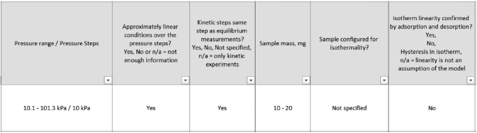
-
-
(5)
Data plotting and model fitting:
-
The way the signal is plotted.
-
Is a model fitting shown on top of the signal?
-
Is the fitting good or poor?
-


Rights and permissions
Open Access This article is licensed under a Creative Commons Attribution 4.0 International License, which permits use, sharing, adaptation, distribution and reproduction in any medium or format, as long as you give appropriate credit to the original author(s) and the source, provide a link to the Creative Commons licence, and indicate if changes were made. The images or other third party material in this article are included in the article's Creative Commons licence, unless indicated otherwise in a credit line to the material. If material is not included in the article's Creative Commons licence and your intended use is not permitted by statutory regulation or exceeds the permitted use, you will need to obtain permission directly from the copyright holder. To view a copy of this licence, visit http://creativecommons.org/licenses/by/4.0/.
About this article

Cite this article
Wang, JY., Mangano, E., Brandani, S. et al. A review of common practices in gravimetric and volumetric adsorption kinetic experiments. Adsorption 27, 295–318 (2021). https://doi.org/10.1007/s10450-020-00276-7
Received:
Revised:
Accepted:
Published:
Issue Date:
DOI: https://doi.org/10.1007/s10450-020-00276-7