
Abstract
We investigate the problem of optimal dividend distribution for a company in the presence of regime shifts. We consider a company whose cumulative net revenues evolve as a Brownian motion with positive drift that is modulated by a finite state Markov chain, and model the discount rate as a deterministic function of the current state of the chain. In this setting, the objective of the company is to maximize the expected cumulative discounted dividend payments until the moment of bankruptcy, which is taken to be the first time that the cash reserves (the cumulative net revenues minus cumulative dividend payments) are zero. We show that if the drift is positive in each state, it is optimal to adopt a barrier strategy at certain positive regime-dependent levels, and provide an explicit characterization of the value function as the fixed point of a contraction. In the case that the drift is small and negative in one state, the optimal strategy takes a different form, which we explicitly identify if there are two regimes. We also provide a numerical illustration of the sensitivities of the optimal barriers and the influence of regime switching.
1 Introduction
A classical topic in finance and actuarial science is that of optimal dividend distribution for a company, which can be phrased as the problem of determining the optimal timing and sizes of dividend payments in the presence of bankruptcy risk, where the usual objective is to maximize the expected value of the cumulative discounted dividend payments until bankruptcy. The earliest work in this setting can be traced back to De Finetti [8] who studied the dividend problem for an insurance company under the binomial model. In continuous time, the problem was posed and solved in a Brownian motion model for the cash reserves by Jeanblanc-Picqué and Shiryaev [20] and Asmussen and Taksar [2], using optimal control theory. Since then an extensive literature has appeared on the dividend problem and its extensions, including reinsurance (e.g. [26]), optimal investment of the reserves (e.g. [18]), tax and proportional cost (e.g. [6, 23]), and growth options (e.g. [7]).
In general, the form of the optimal dividend policy has been found to depend on the expected growth rate and variability of future revenues, and on the discount rate. These quantities will evolve in time, reflecting changing market and economic conditions, and those changes may happen gradually or occur abruptly and be more substantial. Here we focus on the changes of the latter type (also called regime shifts or switches) and model the cumulative net revenues of the company as a Brownian motion with the drift and volatility modulated by a finite state Markov chain, and the discount rate as a deterministic function of the chain. Since Hamilton [16, 17], a substantial econometric literature has appeared that supports the use of Markov regime-switching models to describe business cycles, term structure of interest rates and other macroeconomic quantities. Such models have been shown to be capable of capturing occasional simultaneous and substantial changes of the parameters. Regime-switching models also have the advantage of retaining a degree of analytical tractability, and models from this class can in principle approximate a given diffusion arbitrarily closely by taking the state space large enough and specifying the generator matrix appropriately. In the mathematical finance literature, regime-switching models have become more popular, and have found their applications in stock price models, interest rate models and the real option literature. See e.g. Boyarchenko and Levendorskiǐ [4], Buffington and Elliott [5], Driffill et al. [9], Duan et al. [10], Elliott et al. [12], Guo and Zhang [14], Jiang and Pistorius [21], Naik [24] for derivative pricing, Elliott and van der Hoek [11] and Guidolin and Timmermann [13] for asset allocation, Bäuerle [3], Li and Lu [22], Zhu and Yang [28] and Asmussen [1] for ruin and risk theory, and Guo et al. [15] for irreversible investment.
In this regime-switching setting, we consider the problem of the management of the company to find a dividend distribution policy that maximizes expected discounted dividend payments until bankruptcy, which is defined to occur at the first moment when the level of the cash reserves hits zero. We restrict ourselves to the case that the management can only control the timing and size of the dividend payments. In the case that the drift is positive in every regime, we show that it is optimal to adopt a barrier-type strategy at certain positive levels that depend on the current regime, that is, it is optimal to make the minimal payments needed to keep the cash reserves below these barrier levels. When a regime switch occurs, dividend payments are to be postponed or brought forward in time, according to whether the barrier jumps up or down, and in the latter case a lump sum should be paid if the reserves were above the new barrier at the moment of the switch. In the case of a single regime, this strategy reduces to the classical constant barrier strategy that was found before by Asmussen and Taksar [2].
After an adverse economic regime switch, it could happen that the expected net revenue of the company becomes negative, in which case the optimal strategy takes a different form. Intuitively, it is clear that if the drift is negative and the reserves are sufficiently small, it will be optimal to liquidate the company by paying out the reserves as a lump sum. In the absence of regime switching, this optimality actually holds irrespective of the size of the reserves. In the presence of regime switching, however, we find that it is optimal to continue the business if the drift is small and negative and the reserves are not too small: the prospect of switching to a better regime with suitable positive drift outweighs the risk of ruin. In this case, the value function is not concave, which differs from what is usually found in singular control problems. An explicit solution is derived in Sect. 5 in the case of two regimes.
The dividend optimization problem gives rise to a singular control problem, whose HJB equation takes the form of a coupled system of variational inequalities, due to the fact that the problem is driven by a two-dimensional Markov process. A commonly used direct approach for explicitly solving optimal control problems proceeds by guessing a candidate optimal solution, constructing a corresponding value function, assuming smoothness if necessary, and subsequently verifying its optimality by employing a verification result. Here we follow a different approach to construct the candidate value function, by directly employing a dynamic programming equation. We prove that the value function is the fixed point of a certain contraction operator, which is given explicitly in terms of the initial data, and derive an explicit iterative algorithm to calculate the value function, which ‘decouples’ the different regimes such that, at any stage, one-dimensional control problems are solved. This construction yields in particular that the value function is C 2, which implies that the value function is a classical solution of the HJB equation. At this point, it is worth mentioning that although it is possible to follow the direct approach, this seems to become intractable if the number of states is large, as it leads to a large collection of systems of coupled nonlinear equations (corresponding to different orderings of the dividend levels).
After the first version of this paper was written, we discovered a related work on optimal dividend problems by Sotomayor and Cadenillas [27]. In a setting that is a particular case of ours, with two regimes and constant rate of discounting, they solve three dividend distribution problems with bounded and unbounded dividend rates, and in the presence of fixed cost, respectively, under the assumption of existence of a solution to the smooth fit equation.
The remainder of the paper is organized as follows. In Sect. 2, we give a statement of the problem and present a dynamic programming equation and related theorem. In Sects. 3 and 4, we present the optimal solution and give a proof by constructing an iterative algorithm to calculate the value function V. Section 5 is devoted to a case study of the setting of two regimes, with a numerical illustration of the sensitivities of the optimal barrier levels to the different parameters. Section 6 concludes. Some proofs are presented in the Appendix.
2 Preliminaries and first results
2.1 Problem formulation
Let {W t :t≥0} be a Wiener process and {Z t :t≥0} a continuous time Markov chain with finite state space E and generator matrix Q=(q ij ) i,j∈E , independent of W. Assume that the cash reserves X={X t ,t≥0} evolve, in the absence of dividend payments, as a regime-switching linear Brownian motion, that is, X satisfies the SDE
where Z represents the state of economy. For every state i in E, both drift parameter μ(i) and volatility parameter σ(i)>0 are assumed to be known constants. In case there is no notational confusion possible, we write μ i and σ i for μ(i) and σ(i), respectively. The processes X and Z are defined on some filtered probability space \((\varOmega , \mathcal{F}, \mathbf{F}, \mathbb{P})\) where \(\mathbf{F} =\{\mathcal{F}_{t}, t\geq0\}\) denotes the right-continuous completed filtration jointly generated by X and Z. We denote by ℙ x,i and ℙ x the measure ℙ conditioned on {X 0=x,Z 0=i} and {X 0=x}, respectively, and write \(\mathbb{E}_{x,i}\) and \(\mathbb{E}_{x}\) for the corresponding expectations. We assume that the processes X and Z are both fully observable to the shareholders, and that these decide on the dividend strategies on the basis of the available information.
A dividend strategy D is a nondecreasing and right-continuous stochastic process D={D t :t≥0} with D 0−=0. Here D t represents the cumulative amount of dividends that has been paid out until time t. We assume that, apart from reducing the reserves, dividend payments have no effect on the business and that there are no transaction costs associated to the payment or receipt of dividends. The dynamics of the risk reserve process U={U t :t≥0} in the presence of dividend payments are then given by
for all t until the time τ of bankruptcy and dU t =0 for t after τ, where
is the first time that U hits zero. To avoid degeneracies, only those dividend strategies will be considered that have no lump sum dividend payments larger than the current level of the reserves. A dividend strategy D is called admissible if D is F-adapted, dD t =0 for t≥τ and
Denoting by \(\mathcal{D}\) the set of admissible dividend strategies, the objective function of the shareholders is given by
where V D denotes the expected value of the discounted dividends until the time of ruin τ under the dividend strategy D,
with r:E→(0,∞) the Markov-modulated rate of discounting. The problem for the shareholders is to identify a dividend strategy \(D^{*}\in\mathcal{D}\) that attains the supremum in (2.2), that is, \(V \equiv V_{D^{*}}\).
2.2 A priori bounds
Assume for the moment that there is only a single regime, E={i}. Then we are back in the classical linear Brownian motion setting that was investigated in Asmussen and Taksar [2]. They showed that if μ i >0, the optimal strategy is a constant barrier strategy at the level
According to this strategy, the overflow of the reserves above the level \(a_{i}^{*}\) is immediately paid out as dividends. The corresponding value function is given by
where
and \(\lambda^{-}_{i}<0 < \lambda^{+}_{i}\) denote the roots of the equation \(\frac{1}{2} \sigma_{i}^{2} \lambda^{2}+\mu_{i} \lambda-q=0\), i.e.,
Equations (2.3)–(2.6) show that the value function and optimal level are both functions of the drift and of the rate of discounting per unit of squared volatility. This observation leads one to expect that V(x,i) is bounded above and below by the values V +(x) and V −(x) of firms operating in a more or less favorable environment, with volatility constant equal to one and with drift and discounting equal to \((\frac{\mu_{+}}{\sigma^{2}_{+}},\frac{r_{+}}{\sigma^{2}_{+}}) =(\max_{i\in E}\frac{\mu_{i}}{\sigma^{2}_{i}},\min_{i\in E}\frac{r_{i}}{\sigma^{2}_{i}})\) and \((\frac{\mu_{-}}{\sigma^{2}_{-}},\frac{r_{-}}{\sigma^{2}_{-}}) = (\min_{i\in E}\frac{\mu_{i}}{\sigma^{2}_{i}}, \max_{i\in E}\frac{r_{i}}{\sigma^{2}_{i}})\), respectively. The following result confirms that these explicit bounds indeed hold true.
Proposition 2.1
If μ −>0, we have
for all x≥0,i∈E.
The bounds in (2.7) will be employed in the construction of the optimal value function in Sect. 4.
2.3 Dynamic programming equation and comparison result
The following dynamic programming equation for the value function of the singular control problem (2.2) will form the basis for its solution.
Proposition 2.2
We have
where ζ denotes the epoch of the first regime switch and \(\varLambda _{t} = \int_{0}^{t} r(Z_{s})\,\mathrm{d}s\).
The proof of Proposition 2.2 is given in the Appendix. This dynamic programming equation is associated with the Hamilton–Jacobi–Bellman equation for the value function given by
where ′ denotes the partial derivative with respect to x and \(\mathcal{G}\) denotes the infinitesimal generator of (X,Z), which acts on functions w:[0,∞)×E→[0,∞) with w(⋅,i)∈C 2([0,∞)) for i∈E as \(\mathcal{G}w(x,i) = \mathcal{G}_{o} w(x,i) + \mathcal{G}_{s} w(x,i)\), where
The next result shows that any sufficiently regular supersolution of the HJB equation (2.9) dominates the value function.
Theorem 2.3
Assume that there exists a function w=(w(⋅,i),i∈E), with w(⋅,i), i∈E, C 1 functions on (0,∞) that are piecewise C 2 and satisfy for x>0

Then:
-
(i)
We have w(x,i)≥V(x,i) for all x≥0 and i∈E.
-
(ii)
If in addition w=V D for some \(D\in\mathcal{D}\), then D is an optimal strategy and V≡w.
Proof
(i) Fix an arbitrary \(D\in\mathcal{D}\) and let U be the corresponding risk process. The statement will follow once we have shown that w(x,i)≥V D (x,i). Applying a generalized form of Itô’s lemma to the process \(\{\mathrm{e}^{-\varLambda _{T\wedge\tau}}w(U_{T\wedge\tau},Z_{T\wedge \tau}), T\ge0\}\), we find that

where \(D_{t} = D^{c}_{t} + \sum_{0\leq s\leq t}\varDelta D_{s}\) and (M T∧τ ) is the local martingale with

Here the last integration is over the set [0,t]×[0,N] and \(\widetilde{\pi}= \pi-\nu\) is a compensated random measure,Footnote 1 where \(\pi(\mathrm{d}t,\mathrm{d}j)=\sum_{s\ge0}1_{\{\varDelta Z_{s}(\omega )\neq0\}} \delta_{(s,Z_{s}(\omega ))}(\mathrm{d}t,\mathrm{d}j)\), with δ (s,z) denoting the Dirac measure at the point (s,z), and the compensator ν is given by
where \(p_{Z_{t-}}(j) = \frac{q_{Z_{t-},j}}{-q_{Z_{t-},Z_{t-}}} =P(Z_{t}=j|Z_{t-},\varDelta Z_{t}\neq0)\), where δ is the counting measure on E. Notice from (2.10) that as M is bounded below and M 0=0, M is a supermartingale with \(\mathbb{E}[M_{T\wedge\tau}]\leq0\). In view of the HJB equation (2.9), the first three terms of right-hand side of (2.10) are nonpositive, so that taking expectations yields that
By letting T→∞ and invoking the monotone convergence theorem and the fact that w is nonnegative, we obtain w(x,i)≥V D (x,i) and hence w(x,i)≥V(x,i).
(ii) The equality follows since V D ≤V by definition of V and V D ≥V by part (i). □
3 The optimal dividend strategy
Following the classical approach to solving optimal control problems, we next construct a candidate optimal solution. In view of the fact that (U,Z) is a Markov process, we consider strategies that pay out the overflow of the cash reserves above a regime-dependent level.
Definition 3.1
A modulated barrier strategy at level b=(b(i),i∈E) is a dividend strategy \(D^{b}\in\mathcal{D}\) satisfying

where U b is the risk process (2.1) corresponding to D b.
According to this strategy, dividends are only paid out when U b is at the barrier b, which implies that the process D b is a local time (see Fig 1). It is straightforward to verify that D b can be explicitly expressed in terms of a running supremum as
Employing the heuristic ‘principle of C 2 fit’ of singular control allows us to define candidate optimal levels as the solution of the system of equations
if such a solution exists. In fact, (3.1) follows from Lemma 4.5 and Proposition 4.1 as we shall see later. If the drift is positive in all regimes, this candidate solution is indeed optimal:

Illustrated is the cash reserves process corresponding to a modulated barrier strategy. The barrier levels are represented by horizontal lines. In this case, the barrier jumps down at the moment of the regime switch and a lump sum payment is made
Theorem 3.2
Suppose that we have μ i >0 for all i∈E. Then there exist levels \(b^{*}= (b^{*}_{i}, i\in E)\) with \(0<b^{*}_{i}<\infty\) that solve the system (3.1), and the following holds true:
-
(i)
The optimal value function V is a classical solution of the HJB equation (2.9). In particular, V is equal to the unique solution w={w(x,i),i∈E} with w(⋅,i)∈C 2([0,∞)) of the system
 (3.2)
(3.2)for i∈E, where w i (x)=w(x,i).
-
(ii)
The modulated barrier strategy at b ∗ is an optimal policy in (2.2).

If the positive drift condition is not satisfied, it is not necessarily optimal to adopt a modulated barrier strategy. Indeed, in Sect. 5 we show that in the case of two regimes with a small and negative drift in one state and a positive in the other, the optimal dividend barrier depends on the regime as well as on the level of the reserves. In the following section, we give a proof of Theorem 3.2 by presenting an iterative construction of the optimal value function.
4 Algorithm to compute the value function V
Throughout this section we assume that μ i >0 for all i∈E. We start by observing that the value function V b of a modulated barrier strategy at level b=(b i ,i∈E) solves a fixed point equation in terms of the function \(W_{i}^{(q)}\).
Proposition 4.1
For i∈E, we have
where, for any f:[0,∞)×E→[0,∞),
where θ i =r i −q ii and, for any function f:[0,∞)×E→ℝ, \(A_{i}^{f}\) is given by
The previous result can be utilized to calculate the value function V b of the barrier strategy at b by iterating the map T b :v↦T b v. Denote by \(\mathcal{B}\) the set
where f i =f(⋅,i), and let \(\|f\| =\max_{i\in E}\sup_{x\ge0}\frac{|f_{i}(x)|}{1+|x|}\) for \(f\in\mathcal{B}\).
Corollary 4.2
The map T b is a contraction on \(\mathcal{B}\) with respect to the norm ∥⋅∥. In particular, for \(f\in\mathcal{B}\) we have
where the convergence is in ∥⋅∥-norm and \(T^{n}_{b}(f) = T_{b}(T^{n-1}_{b}(f))\) for n>1 with \(T^{1}_{b}=T_{b}\).
Proof of Proposition 4.1
Denote by U i=X i−D i the risk process corresponding to dividends D i being paid according to a constant barrier strategy at b i , with \(X^{i}_{t}=x+\mu_{i}t + \sigma_{i} W_{t}\). Let \(\tau^{b}=\inf\{t\ge0:U_{t}^{b}<0\}\) and \(\tau^{i} = \inf\{t\ge0: U^{i}_{t}<0\}\) be the ruin times of U b and U i, and denote by ζ the epoch of the first regime switch and by η(a) an independent exponential random time with mean 1/a. Then we find that the ensemble (U t ,Z 0=i,t<τ b∧ζ) is in distribution equal to \({(U^{i}_{t},t<\tau^{i}\wedge\eta(-q_{ii}))}\). Thus, the value z 1(x,i) of the discounted dividends received before ζ is given by

where θ i =r i −q ii and in the last line we used (2.4). Similarly, the value z 2(x,i) of the discounted dividends received after ζ satisfies, in view of the Markov property,

Employing the identity (see e.g. Pistorius [25], Theorem 1) for x∈[0,b i ]

and the fact that V b(x,i)=z 1(x,i)+z 2(x,i), we find the result as stated. □
Proof of Corollary 4.2
Note that \(\mathcal{B}\) endowed with the norm ∥ ⋅ ∥ is a complete metric space and that T maps \(\mathcal{B}\) to itself, by definition of T and the fact that \(W^{(\theta_{i})}_{i}\) is C 1. Subsequently we see that

where h i is given in (4.4) (with b replaced by b i ) and \(C = \max_{i}\sum_{j\neq i}\frac {q_{ij}}{\theta_{i}}< 1\). Here we used that \(\int_{0}^{b_{i}} h_{i}(x,y)\,\mathrm{d}y = 1 -\mathbb{E}_{x,i}[\mathrm{e}^{-\theta_{i}\tau^{i}}]\). Thus it follows that T is a contraction on \(\mathcal{B}\), which implies the convergence in (4.3). □
4.1 Iteration
In a next step, we consider the auxiliary control problem with a prescribed payoff function v to be received at the epoch of the first regime switch ζ, i.e.,
This singular control problem can be solved explicitly if v lies in the set of smooth concave payoff functions \(\mathcal{C} =\{v\in\mathcal{B}: \text{$v_{i}$ is increasing and concave}, i\in E\}\).
Proposition 4.3
Let \(v\in\mathcal{C}\). Then Uv(⋅,i)∈C 2[0,∞) for i∈E, and the optimal strategy in (4.5) is given by a regime-switching barrier strategy at the levels \(b^{v}=(b^{v}_{i}, i\in E)\), \(0<b^{v}_{i}<\infty\), given by
with A v given in (4.2).
Supposing that the map U:v↦Uv preserves concavity and smoothness, this proposition can be applied iteratively, as follows: Initialize by setting n=0 and v=v 0 for some \(v_{0}\in\mathcal{B}\) and then
-
(1)
find \(b^{v}=(b^{v}_{i},i\in E)\) in (4.6);
-
(2)
set \(v \leftarrow T_{b^{v}}(v)\), n←n+1 and v n ←v, and return to step (1).
The following result shows that the sequence (v n ) generated in this way converges to the value function V as n→∞.
Proposition 4.4
Let \(v_{0}^{\pm}\in\mathcal{C}\) and define \(v_{n}^{\pm}= Uv^{\pm}_{n-1}\) for n≥1. If \(v_{0}^{-}\leq V\leq v_{0}^{+}\), then \(v_{n}^{-} \leq V\leq v_{n}^{+}\) and
where the convergence is with respect to the norm ∥⋅∥. In particular, V is concave.
In fact, we shall show below that U is a contraction on \(\mathcal{C}\). Notice that Theorem 3.2(i) is now a direct consequence of these results. Indeed, by combining Proposition 4.3 and the dynamic programming equation (2.8), we see that the optimal strategy in (2.2) is given by a modulated barrier strategy at some positive finite levels. Explicit examples of initial functions \(v_{0}^{\pm}\) are the V ± given in Proposition 2.1.
4.2 Proofs
This subsection is devoted to the proofs of Propositions 4.3 and 4.4, which we split into a number of steps. The first step is to verify that the \(b^{v}_{i}\) as defined above are positive and finite, which is a matter of straightforward calculations using the explicit expression (2.5).
Lemma 4.5
(Existence of optimal barrier levels)
Let \(v\in\mathcal{C}\). Then \(b\mapsto A^{v}_{i}(b)\) attains its maximum at some finite and positive b i , which satisfy
In particular, \(T_{b^{v}}(\cdot, i)\in C^{2}[0,\infty)\) for i∈E.
The proof of Lemma 4.5 is given in the Appendix. The key step is to verify next that the value function of a barrier strategy at level b v with a concave payoff function v(⋅,i) is itself concave.
Lemma 4.6
(Preservation of concavity)
If \(v\in\mathcal{C}\), then \(T_{b^{v}}(v)\in\mathcal{C}\).
Proof
We first assume that \(v\in\mathcal{C}\cap C^{2}[0,\infty)\), and write b instead of b v to simplify the notation. In view of the smoothness of v and the definition of \(w_{i}(x):=(T_{b^{v}}v)(x,i)\), we can obtain from (2.5) and (4.1) that for x∈(0,b i ),
and

From these expressions, (2.5) and v∈C 2[0,∞), we have \(w_{i}|_{(0,b_{i})}\in C^{4}(0,b_{i})\). In addition, we have \(w_{i}'(b_{i})=1\) from the above expressions and (4.1), and \(w_{i}''(b_{i})=0\) by Lemma 4.5. As a result, w i is in C 2[0,∞).
An application of Itô’s lemma shows that w i satisfies the ODE, for x∈(0,b i ),
with boundary conditions \(w_{i}(0)=0, w_{i}'(b_{i}) = 1\). Since w i (x)≥0 for x>0 and w i (0)=0, we deduce that \(w_{i}'(0+)\ge 0\). Furthermore, the continuity of w i and the fact that w i (0)=0 and v i (0)=0 imply that
so that \(w_{i}''(0+)<0\), as μ i >0 by assumption.
Write now \(\xi_{i}(x)=w_{i}''(x)\) for x>0, and denote \(\xi_{i}(0)=w_{i}''(0+)\). By twice differentiating the first equation of the original system (3.2), which is justified since w i (x)∈C 4(0,b i ) as a consequence of the assumptions, we find that ξ i (x) satisfies the ODE
Another application of Itô’s lemma then yields for ξ the representation
where θ i =(c i −q ii ) and \(T^{i} = \inf\{t\ge0:X^{i}_{t}\notin(0,b_{i})\}\). Thus, since \(\xi_{i}(X_{T^{i}})\leq0\) and \(v_{j}''(x)\leq0\), it follows that ξ i (x) is nonpositive for all x∈(0,b i ) and i∈E. In particular, we deduce that x↦w i (x) is concave and increasing on [0,∞).
Suppose now that \(v\in\mathcal{C}\) and let \(v_{n}\in\mathcal{C}\cap C^{2}[0,\infty)\) be a sequence that pointwise increases to v. Then \(T_{b^{v}}(v)(x,i) = \lim_{n\to\infty} T_{b^{v}}(v_{n})(x,i)\), and the concavity of \(T_{b^{v}}(v)\) directly follows from the fact that the pointwise limit of concave functions is concave. □
We next verify that the modulated barrier strategy at b v is optimal for the problem (4.5).
Lemma 4.7
(Optimality of barrier strategies)
For \(v\in\mathcal{C}\), we have for x>0,i∈E that \(T_{b^{v}}(v)(x,i) = Uv(x,i)\).
Proof
Defining again \(w_{i}(x) = T_{b^{v}}(v)(x,i)\) and \(f_{i}^{v}(x)\) as in (4.7), we shall verify that \(f^{v}_{i}(x)\leq0\) for x>b i . Next we claim that
The claim (4.8) is proved as follows. From the facts that \(w_{i}''(b_{i})=0\) and \(w_{i}''(x)\leq0\) for x<b i (as a consequence of the concavity of w i ), it follows that \(w_{i}'''(b_{i}-)\geq0\). Since both \(w_{i}''(x)\) and \(w_{i}'(x)\) are continuous at x=b i and \(w_{i}'''(b_{i}+)=0\), it follows by considering the left and right limits of \(f^{v\prime}_{i}(x)\) at x=b i that \(f^{v\prime}_{i}(b_{i}-)\geq f^{v\prime}_{i}(b_{i}+)\). Finally, differentiating the identity \(f^{v}_{i}(x)\equiv0\) for x∈(0,b i ) shows \(f^{v\prime}_{i}(b_{i}-)=0\) and thus (4.8) follows.
Noting that \(f^{v\prime}_{i}(x) = -(c_{i}-q_{ii}) + \sum_{j\in E}q_{ij}v_{j}'(x)\) for x>b i , the concavity of v together with (4.8) yields then that \(f^{v\prime}_{i}(x)\leq f^{v\prime}_{i}(b_{i}+)\leq0\) for x>b i , which implies that \(f^{v}_{i}(x)\leq0\) for x≥b i (noting that \(f^{v}_{i}(b_{i})=0\), by continuity).
Since the w i are C 2 and concave and satisfy (4.7), the assertion of the lemma follows by an argument similar to the one used in the proof of Theorem 2.3. Fix an arbitrary \(D\in\mathcal{D}\) and let U be the corresponding risk process. Applying a generalized form of Itô’s lemma to the process \(\{\mathrm{e}^{-\varLambda _{T\wedge\tau}}w(U_{T\wedge\tau},Z_{T\wedge\tau}), T\ge0\}\), taking expectations and using that \(f^{v}_{i}(x)\leq0\) as in the proof of Theorem 2.3, we find that

By letting T→∞ and invoking the monotone convergence theorem and the fact that w and v are nonnegative and \(f^{v}_{i}(x)\leq0\), we obtain w(x,i)≥Uv(x,i). Since the barrier strategy at level b v is an element of \(\mathcal{D}\), it also holds that Uv(x,i)≥w(x,i), so that w(x,i)=Uv(x,i). □
The convergence of the iteration procedure is an immediate consequence of the following contraction property of Uv.
Lemma 4.8
(Contraction)
The map v↦Uv is a contraction on \(\mathcal{C}\) with respect to ∥⋅∥.
Proof
By Lemmas 4.7 and 4.6, we have \(Uv(x,i) = \sup_{b}T_{b}(v)(x,i) = (T_{b^{v}}v)(x,i)\) and \(Uv\in\mathcal{C}\) for \(v\in \mathcal{C}\). Hence it follows that for \(v,w\in\mathcal{C}\),
where C<1 and the second inequality follows as in the proof of Corollary 4.2. Thus U is a contraction on \(\mathcal{C}\). □
Proof of Propositions 4.3 and 4.4
Proposition 4.3 directly follows by combining Lemma 4.5 with Lemma 4.7.
From the definition of U and the dynamic programming equation, we directly see that Uv≤V≤Uw if v≤V≤w. In particular, taking \(v=v_{0}^{-}\) and \(w=v_{0}^{+}\) and repeatedly applying the former inequality yields that \(v_{n}^{-}\leq V\leq v_{n}^{+}\). It follows from Lemma 4.8 that \((v_{n}^{+})\) and \((v_{n}^{-})\) converge to the unique fixed point of U, which is therefore equal to V. Next note that in view of Lemma 4.6, \(v_{n}^{\pm}\) are concave (as we took \(v_{0}^{\pm}\in \mathcal{C}\)), so that V, a pointwise limit of concave functions, is also concave. This completes the proof of Proposition 4.4. □
5 Case study: two regimes
5.1 Positive drifts
From now on, we restrict ourselves to the case of two regimes, E={0,1}. For the setting of positive drifts, μ 0,μ 1>0, we derive a system of two nonlinear equations for the optimal dividend barriers. We denote by F 0 and F 1 the quadratic polynomials given by
with two different real roots \(\lambda_{1}^{k}\) and \(\lambda_{2}^{k}\). Consider the fourth order polynomial
The equation F k (λ)=0 has two different roots \(\lambda_{-}^{k}<\lambda_{+}^{k}\) given in (2.6), and the equation F 0,1(λ)=0 has four real roots satisfying λ 1<λ 2<0<λ 3<λ 4.
Solving the systems of differential equations in Theorem 3.2 leads to the following result:
Proposition 5.1
Suppose that μ 0,μ 1>0 and let \(b_{0}^{*} < b_{1}^{*}\). Then \((b_{0},b_{1})=(b^{*}_{0},b^{*}_{1})\) solve the two nonlinear equations

where d=(d 1,…,d 4)′ solves the linear system Ad=h, where h=(0,0,1,0)′ and
The proof of Proposition 5.1 is given in the Appendix.
5.1.1 Sensitivities of the optimal barriers
To illustrate the effects of regime switching and the sensitivities of the optimal barrier levels, we numerically solved the system of nonlinear equations in Proposition 5.1 for different parameter values, and compared the results with the explicit solutions (2.3) and (2.4) corresponding to the absence of regime switching. The nonlinear equations were solved using a Maple routine based on the standard quasi-Newton method. We chose the parameters as in Table 1 and varied μ 0, σ 0, q 00 and r 0 individually while keeping the other parameters fixed—the results are given in Table 2.
We see that when the drift parameter μ 0 is increased, then initially \(b^{*}_{0}\) and \(b^{*}_{1}\) increase, while they decrease when the drift μ 0 becomes very large. Apparently, for relatively low drift it is optimal to reduce the probability of ruin, while for large drift the effect of discounting takes priority. Table 2 also shows that the two barriers \(b^{*}_{0}\) and \(b^{*}_{1}\) monotonically increase when σ 0 increases. A larger volatility leads to a higher probability of ruin, requiring the company to raise the level of the barrier in order to protect its future operations. We can also observe the effect of the transition rates of the underlying Markov chain. For example, if the rate is −q 00=0.01, the chain spends a large part of the time in state 0 (in equilibrium, 3/3.01≈99.7% of the time), which we find back as \(b^{*}_{0}=1.014\) is very close to \(a_{0}^{*}=1.013\), whereas if −q 00 and −q 11 are of similar size, the chain spends on average similar amounts of time in both states and the level \(b^{*}_{0}\) differs substantially from \(a_{0}^{*}\). Finally, we note that both \(b^{*}_{0}\) and \(b^{*}_{1}\) decrease when the rate of discounting r 0 is increased; if the rate of discounting is higher, it is optimal to increase the dividend payments by lowering the dividend barriers.
5.2 Adverse regime shifts: negative drift
We next consider the case that the drift is positive in one state and negative in the other. Intuitively, it is clear that for sufficiently small reserves a quick bankruptcy of the company is quite likely if the drift is negative, so that it is optimal to liquidate the company by paying out the entire reserves as a lump sum. If, however, the negative drift is moderate and the reserves are not too small, the expected future gains from a regime switch to a ‘good’ state may outweigh the effect of the negative drift, and it may be optimal to continue the business. In that case, a sensible strategy could be to liquidate the company for small initial reserves, but to pay out dividends according to a modulated barrier strategy for larger levels of reserves, which we formalize as follows.
Definition 5.2
A modulated liquidation and dividend barrier strategy at levels d=(d(i),i∈E) and b=(b(i),i∈E) is a dividend strategy \(D^{d,b}\in\mathcal{D}\) satisfying

where U d,b is the insurance risk process (2.1) corresponding to D d,b.
Condition (iii) states that all the reserves are paid out as dividends once the risk reserves fall below the level d(Z t ). Define next the critical levels
where Y i (x):=μ i −c i x+∑ j≠i q ij (V j (x)−x). Note that if μ i <0, Y i (x) is negative for all x small enough, which implies that Δ i ∈(0,∞]. If Δ i =+∞, which is the case if μ i <0 and |μ i | is sufficiently large, it is optimal in state i to liquidate the company for any level of the reserves, by immediately paying out all the reserves as dividends—this can be directly checked from Theorem 2.3. In the case that μ 0<0<μ 1 and Δ 0<∞ (the case μ 1<0<μ 0 follows by relabeling the states), it turns out that it is optimal to continue paying dividends if the reserves are large enough, where the ‘liquidation’ level \(d^{*}_{0}>0\) solves the smooth fit equation \(V_{0}'(d^{*}_{0}) = 1\). The solution is explicitly given as follows.
Proposition 5.3
Suppose that μ 0<0<μ 1 and Δ 0<∞.
-
(i)
The optimal strategy in (2.2) is given by the modulated liquidation and dividend barrier strategy at levels \(d^{*}=(d^{*}_{0},0)\) and \(b^{*}=(b^{*}_{0},b^{*}_{1})\) that solve the system
$$V_0'\bigl(d^*_0\bigr) = 1,\qquad V_0''\bigl(b^*_0\bigr)=0,\qquad V_1''\bigl(b_1^*\bigr)=0.$$ -
(ii)
If \(b^{*}_{1}<b^{*}_{0}\), then \(d^{*}_{0},b^{*}_{0}\), and \(b^{*}_{1}\) solve the system of nonlinear equations

where \(\epsilon_{i,j} = \mathrm{e}^{\lambda_{i}^{1}d_{0}}[(\lambda^{1}_{i})^{2} -\lambda_{i}^{1}\lambda_{j}]\), \(\phi= (\lambda_{1}^{1})^{2}\mathrm{e}^{\lambda_{1}^{1}d_{0}}- (\lambda_{2}^{1})^{2}\mathrm{e}^{\lambda_{2}^{1} d_{0}}\), and B=(B 1,…,B 4)′ solves the linear system
$$ A^* B= h,$$with h=(d 0,1,q 00,0)′ and \(A^{*}=(A^{*}_{1}, A^{*}_{2}, A^{*}_{3}, A^{*}_{4})\) with columns given by
$$A^*_i= \left(\begin{array}{c}\exp(\lambda_i d_0)\\\lambda_i\exp(\lambda_i d_0)\\ F_0(\lambda_i) \lambda_i \exp(\lambda_i b_1)\\F_0(\lambda_i) \lambda_i^2\exp(\lambda_i b_1)\end{array} \right) \quad i=1,2,3,4.$$The value functions are given by
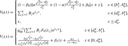
where \(\alpha= \frac{\lambda_{2}^{0}}{\lambda_{2}^{0}-\lambda_{1}^{0}}\), \(\beta_{i} = \frac{-q_{ii}}{c_{i}-q_{ii}}\) and


The proof is given in the Appendix. Observe that the value function V 0 is not concave, as there are two disjoint intervals where it has unit slope.
As illustration, we provide next a numerical example of a case where a modulated liquidation-dividend strategy is optimal.
Example
Consider the case where μ 0=−0.08, σ 0=0.40, q 00=−10, c 0=0.06, μ 1=0.14, σ 1=0.50, q 11=−0.001 and c 1=0.08. Numerically solving the system of nonlinear equations in Proposition 5.3, we obtained that d 0=0.086, b 0=1.418 and b 1=1.415, and that the value functions V 0 and V 1 (plotted in Fig. 2) are given by
and

The value function V 0(x) and the corresponding optimal dividend barriers d 0,b 0,b 1 in the case where the parameters are μ 0=−0.08, σ 0=0.40, q 00=−10, c 0=0.06, μ 1=0.14, σ 1=0.50, q 11=−0.001, c 1=0.08. Note that V 0 is not concave
6 Conclusion
In this paper, we have shown that in the presence of regime shifts, the optimal dividend policy is given by a threshold strategy set at a level that is a function of the current regime. That is to say, the policy that maximizes the expectation of the net present value of the paid dividends until the moment of default consists of paying out as dividends the overflow of the cash reserves above a certain optimal threshold, where this threshold jumps up or down exactly at the moment when the regime shifts. Hence, at the moment of a regime shift when the key parameters such as drift, volatility and discounting may change, it may be optimal to make a lump sum dividend payment, namely when the threshold level jumps below the current level of the cash reserves. We presented a contraction algorithm for the computation of the optimal threshold levels. As a case study, we numerically investigated the parameter sensitivities of the levels in the case of two regimes. It would be desirable to systematically explore the dependence of the optimal threshold levels on key parameters and its financial significance, which could be achieved by an analytical investigation of its form in specific parametric models; this is a topic left for future research.
Notes
See e.g. Jacod and Shiryaev [19, II.1.16] for background on random measures.
References
Asmussen, S.: Risk theory in a Markovian environment. Scand. Actuar. J. 2, 69–100 (1989)
Asmussen, S., Taksar, M.: Controlled diffusion models for optimal dividend pay-out. Insur. Math. Econ. 20, 1–15 (1997)
Bäuerle, N.: Some results about the expected ruin time in Markov-modulated risk models. Insur. Math. Econ. 18, 119–127 (1996)
Boyarchenko, S., Levendorskiǐ, S.: Exit problems in regime-switching models. J. Math. Econ. 44, 180–206 (2008)
Buffington, J., Elliott, R.J.: American options with regime switching. Int. J. Theor. Appl. Finance 5, 497–514 (2002)
Cadenillas, A., Sarkar, S., Zapatero, F.: Optimal dividend policy with mean-reverting cash reservoir. Math. Finance 17, 81–109 (2007)
Décamps, J.P., Villeneuve, S.: Optimal dividend policy and growth option. Finance Stoch. 11, 3–27 (2007)
De Finetti, B.: Su un’impostazione alternativa dell teoria colletiva del rischio. In: Transactions of the XV International Congress of Actuaries, vol. 2, pp. 433–443 (1957)
Driffill, J., Kenc, T., Sola, M.: Merton-style option pricing under regime switching. Comput. Econ. Finance 304 (2002). http://www.econpapers.repec.org/paper/scescecf2/304.htm
Duan, J.C., Popova, I., Ritchken, P.: Option pricing under regime switching. Quant. Finance 2, 1–17 (2002)
Elliott, R.J., van der Hoek, J.: An application of hidden Markov models to asset allocation problems. Finance Stoch. 1, 229–238 (1997)
Elliott, R.J., Siu, T.K., Chan, L.L.: Pricing volatility swaps under Heston’s stochastic volatility model with regime switching. Appl. Math. Finance 14, 41–62 (2007)
Guidolin, M., Timmermann, T.: International asset allocation under regime switching, skew, and kurtosis preferences. Rev. Financ. Stud. 21, 889–935 (2008)
Guo, X., Zhang, Q.: Closed-form solutions for perpetual American put options with regime switching. SIAM J. Appl. Math. 64, 2034–2049 (2004)
Guo, X., Miao, J., Morellec, E.: Irreversible investment with regime shifts. J. Econ. Theory 122, 37–59 (2005)
Hamilton, J.D.: A new approach to the economic analysis of non-stationary time series and the business cycle. Econometrica 57, 357–384 (1989)
Hamilton, J.D.: Analysis of time series subject to changes in regime. J. Econom. 45, 39–79 (1990)
Højgaard, B., Taksar, M.: Optimal risk control for a large corporation in the presence of returns on investments. Finance Stoch. 5, 527–547 (2001)
Jacod, J., Shiryaev, A.N.: Limit Theorems for Stochastic Processes, 2nd edn. Springer, Berlin (2003)
Jeanblanc-Picqué, M., Shiryaev, A.N.: Optimization of the flow of dividends. Russ. Math. Surv. 50, 25–46 (1995)
Jiang, Z., Pistorius, M.R.: On perpetual American put valuation and first passage in a regime-switching model with jumps. Finance Stoch. 12, 331–355 (2008)
Li, S.M., Lu, Y.: Moments of the dividend payments and related problems in a Markov-modulated risk model. N. Am. Actuar. J. 11, 65–76 (2007)
Løkka, A., Zervos, M.: Optimal dividend and issuance of equity policies in the presence of proportional costs. Insur. Math. Econ. 42, 954–961 (2008)
Naik, V.: Option valuation and hedging strategies with jumps in the volatility of asset returns. J. Finance 48, 1969–1984 (1993)
Pistorius, M.R.: On exit and ergodicity of the spectrally one-sided Lévy process reflected at its infimum. J. Theor. Probab. 17, 183–220 (2004)
Schmidli, H.: Optimal proportional reinsurance policies in a dynamic setting. Scand. Actuar. J. 101(1), 55–68 (2001)
Sotomayor, L.R., Cadenillas, A.: Classical, singular, and impulse stochastic control for the optimal dividend policy when there is regime switching. Insur. Math. Econ. 48, 344–354 (2011)
Zhu, J., Yang, H.: Ruin theory for a Markov regime-switching model under a threshold dividend strategy. Insur. Math. Econ. 42, 311–318 (2008)
Acknowledgements
We thank A. Dassios, R. Norberg, M. Zervos, participants of the 12th International Congress of IME (Insurance: Mathematics and Economics) in Dalian, China, and the Bachelier Conference in London (July 2008) for useful suggestions. We are grateful to Chengming Xu and two anonymous referees for helpful comments and a careful reading of the paper.
Research supported by EPSRC grant EP/D039053. The research was carried out in part while the authors were based at King’s College London.
Open Access
This article is distributed under the terms of the Creative Commons Attribution License which permits any use, distribution, and reproduction in any medium, provided the original author(s) and the source are credited.
Author information
Authors and Affiliations
Corresponding author
Additional information
This paper is based on Chap. 3 of the first author’s PhD thesis.
Appendix: Proofs
Appendix: Proofs
1.1 A.1 Proof of the bounds (Proposition 2.1)
To prove the upper and lower bounds in (2.7), we consider two auxiliary optimal switching problems where not only the dividend payout, but also the regime is a control variable. An admissible switching strategy \(\sigma=\{Z^{\sigma}_{t}, t\ge0\}\) is an F-adapted E-valued process that indicates the current regime. The two control problems are then given by
where D − denotes the constant barrier strategy at level b − (where b − denotes the optimal barrier corresponding to V −), \(\mathcal{S}\) and \(\mathcal{D}\) are the sets of all admissible switching and dividend strategies, \(\varLambda ^{\sigma}_{s}=\int_{0}^{s}c(Z_{u}^{\sigma})\,\mathrm{d}u\), and τ σ is the corresponding ruin time. As the regime-switching process Z is one particular admissible switching strategy, the upper and lower bounds in (2.7) will follow once we have shown that v +≤V + and v −≥V −.
In the proof, we use the following sub- and super-harmonicity properties:
Lemma A.1
For all i∈E, we have


where \(\mathcal{G}_{i}\) is the infinitesimal generator of \(X^{i}_{t}=x + \mu_{i}t + \sigma_{i} W_{t}\).
Proof
Since V + is the value function corresponding to the optimal dividend problem without regime switching and with volatility, drift and discounting given by 1, \(\max_{i\in E}\frac{\mu_{i}}{\sigma^{2}_{i}}\), \(\min_{i\in E}\frac{c_{i}}{\sigma^{2}_{i}}\), it solves a corresponding HJB equation. In particular, \(V_{+}'\) and V + are both positive so that in view of the form of the drift and discounting, it follows that (A.1) holds true. By a similar argument, it can be verified that (A.2) holds true. □
Proof of Proposition 2.1
Fixing arbitrary admissible switching and dividend strategies σ and D and denoting by U σ,D the corresponding risk process, an application of Itô’s lemma shows that

where M σ is some local martingale which is a supermartingale as it is bounded below. Taking note of Lemma A.1 and the facts that \(V_{+}^{\prime}\ge1\) and V +(0)=0, it follows by rearranging and taking expectations that
Subsequently taking the supremum in (A.3) over all \(\sigma\in\mathcal{S}\) and \(D\in\mathcal{D}\) shows that V +(x)≥v +(x). By a similar line of reasoning, it can be verified that V −(x)≤v −(x) for all x≤b −. In particular, writing χ=(b −,…,b −), it follows that for all x≤b −,
Observing that, for x≥b −, V −(x)′=1 whereas \((V^{\chi}_{i})^{\prime}(x)\ge1\), we see that (A.4) is valid for all x≥0, and since V χ≤V, the proof of (2.7) is complete. □
1.2 A.2 The dynamic programming equation (Proposition 2.2)
The proof is an adaptation of a classical line of reasoning to a regime-switching setting. We start with the following two lemmas.
Lemma A.2
For x≥y≥0 and i∈E, we have
where θ i =c i −q ii In particular, it follows that V(⋅,i) is Lipschitz-continuous.
Proof
Let ϵ>0 and let D(u,i) be an ϵ-optimal strategy for U 0=u,Z 0=i, and consider the strategies \(D'_{t}(u,y) =(u-y)\mathbf{1}_{\{t=0\}} + D_{t}(y,i)\mathbf{1}_{\{t>0\}}\) (“pay a lump sum u−y and follow then the strategy D(y,i)”) and \(\tilde {D}_{t}(u,x)=\mathbf{1}_{\{t>\tau(x), Z_{\tau(x)}=i\}}D(x,i)\) for x≥u≥y (“wait until the first time τ(x) that the reserves reach the level x; if no regime switch has occurred by then, follow the strategy D(x,i), otherwise don’t pay any dividends”). Then it follows that

where \(t_{i}(y,x) = E_{y}[\mathrm{e}^{-\theta_{i} \tau(x)}\mathbf{1}_{\{\tau (x)<\tau\}}] =\frac{W^{(\theta_{i})}(y)}{W^{(\theta_{i})}(x)}\). Letting ϵ→0, the bounds follow. □
Lemma A.3
Let M>0,ϵ>0. There exists a \(\widetilde{D}\in\mathcal{D}\) such that
Proof
Choose a grid \((x_{(j)}:= \frac{jM}{N}, j=0, \ldots, N)\) of [0,M], where N<ϵ −1 is chosen such that max i∈E m V,i (N −1)<ϵ, with m V,i the modulus of continuity of V(⋅,i), i.e.,
Let D i,j be ϵ-optimal strategies corresponding to U 0=x (j) and Z 0=i, that is, \(V(x_{(j)},i) -V_{D^{i,j}}(x_{(j)},i) < \epsilon\), and define the strategy \(\widetilde{D}\) depending on U 0=x and Z 0=i as “pay a lump sum \((x-x_{(j^{*})})\) and follow then the strategy \(D^{i,j^{*}}\)”, where j ∗=max{j:x (j)≤x}, i.e.,
Then it follows that

As this estimate holds for arbitrary x≥0 and i∈E, the proof is complete. □
Proof of Proposition 2.2
Denote by w the right-hand side of (2.8) and by \(D\in\mathcal{D}\) and U an arbitrary admissible strategy and the corresponding cash reserves. To show that V≤w, we verify that V D ≤w; indeed,

To prove the opposite bound w≤V, we show that for given ϵ>0 and \(D\in\mathcal{D}\), there exists a strategy \(D(\epsilon)\in\mathcal{D}\) such that w D ≤V D(ϵ)+const ϵ, where w D denotes the expectation in (2.8). Fixing M>0 such that P x,i (X ζ>M)<ϵ for all i∈E, we denote by \(D^{\epsilon}\in\mathcal{D}\) a dividend strategy that pays out x−M if U 0=x>M, and that is ϵ-optimal, uniformly over starting values (i,x)∈E×[0,M], that is, we have \(V(x,i)<V_{D^{\epsilon}}(x,i) +\epsilon\) for all (i,x) in this set. Letting θ denote the shift operator, note that the strategy \(D(\epsilon):=D_{t}\mathbf{1}_{\{t<\zeta\}}+ (D^{\epsilon}_{t-\zeta} \circ\theta_{\zeta}) \mathbf{1}_{\{t\ge\zeta\}}\) is in \(\mathcal{D}\), and that it satisfies

where C=max i (V(x,i)−x), which is finite in view of Proposition 2.1. □
1.3 A.3 The optimal levels (Lemma 4.5)
Proof of Lemma 4.5
By straightforward calculus, it can be verified that its derivative is given by
where \(k_{i}(y,b) = W^{(q)\prime}_{i}(y) - W_{i}^{(q)}(y)\ell^{(q)}_{i}(b)\) with \(\ell^{(q)}_{i}(b)=W^{(q)\prime\prime}_{i}(b)/W^{(q)\prime}_{i}(b)\) and q=θ i . From (2.5), it is straightforward to check that \(\ell^{(q)}_{i}(b)\) converges to \(\lambda_{i}^{+}(q)\) as b→∞, and that \(k_{i}(y,b) \leq2{\sigma^{-2}_{i}}\mathrm {e}^{\lambda ^{-}_{i}(q) y}\). By dominated convergence, it then follows that \(W^{(q)\prime}_{i}(b)A^{v\prime}_{i}(b)\) tends to \(-\lambda^{+}_{i}(q) <0\) as b→∞. Since it also holds that \(A^{v\prime}_{i}(0+) =4\mu_{i}/\sigma^{4}_{i} > 0\), we see that \(A^{v}_{i}(b)\) attains its maximum on (0,∞). Therefore \(A_{i}^{v\prime}(b_{i})=0\) which implies that \((T_{b}v)^{\prime\prime}_{i}(b_{i})= 0\), in view of the definition of T b v. Since T b v″(x,i)=0 for x>b i , it follows that \(T_{b^{v}}(\cdot,i)\in C^{2}[0,\infty)\) for i∈E. □
1.4 A.4 The case of two regimes (Propositions 5.1 and 5.3)
Lemma A.4
If there exist 0<b ı <b ȷ such that the system (3.2) holds true, then

Proof
When 0<b ı <x<b ȷ , it follows immediately from (3.2) that
whose general solution is of the form
for any k 1, k 2∈ℝ, since the quadratic characteristic equation F ȷ (λ)=0 of its corresponding homogeneous equation has two roots \(\lambda_{1}^{\jmath}\) and \(\lambda_{2}^{\jmath}\), and its particular solution is obviously k 3 x+k 4, where
Using the boundary conditions \(\frac{\partial V(x,\jmath)}{\partial x}|_{x=b_{\jmath}} =1\) and \(\frac{\partial^{2} V(x,\jmath)}{\partial^{2} x}|_{x=b_{\jmath}}=0\) then yields
The proof is complete. □
Proof of Proposition 5.1
In view of Lemma A.4, to complete the proof, it remains to derive the system. For 0<x<b ı <b ȷ , it follows from (3.2) that V(x,ı) satisfies a fourth order linear homogeneous ordinary differential equation with the characteristic equation F 0(λ)F 1(λ)−q 00 q 11=0 having four real roots λ 1<λ 2<λ 3<λ 4. Thus, for 0<x<b ı , V(x,ı) and V(x,ȷ) can be, respectively, expressed as


where the coefficients d i ,i=1,…,4, are to be determined. By expressing the boundary conditions
in terms of these coefficients, we arrive at the matrix equation Ad=h. The equations for the optimal levels follow since V(x,ȷ) is C 2 at b ı (noting that any two of the three equations implies the third one). □
The system in Proposition 5.1 can be solved explicitly, as shown in the following result. To that end, we introduce the functions \(\tilde{g}_{\imath,k}\) and g ı,k , k=1,2, via

where \(C_{k} = \frac{F_{\imath}(\lambda_{k})-F_{\imath}(\lambda_{4})}{F_{\imath}(\lambda_{4})-F_{\imath}(\lambda_{3})}\), and we write
Lemma A.5
If G≠0, we have for 0≤x<b ı

Proof
From the first two equations of the system Ad=h and in view of μ ı >0 and λ 4>λ 3>0, we can express the coefficients d 3 and d 4 in terms of d 1 and d 2 by
Substituting this into (A.5) and (A.6) yields

The last two equations of Ad=h can then be rewritten as
with a unique solution
according to Cramér’s rule (as G≠0). □
Proof of Proposition 5.3
The structure of the proof is analogous to that of Theorem 3.2. As the value function V 0 will not be concave, some parts of the proof have to be modified. The steps are outlined as follows:
(1) The value function of a modulated liquidation-dividend strategy V d,b satisfies \(V = \tilde{T}_{d,b} V\), where
where θ i =c i −q ii , \(Z_{i}^{(\theta_{i})}(x)=1+\theta_{i}\int_{0}^{x} W^{(\theta_{i})}_{i}(y)\,\mathrm{d}y\) and

(2) The map \(f\mapsto\sup_{d,b}\tilde{T}_{d,b}f\) is a contraction on \(\mathcal{B}\). As a consequence, there exists a function w with \(w=\sup_{d,b}\tilde{T}_{d,b}w\). By similar arguments as used in Lemma 4.5, it can be verified that there exist d 0,b 0,b 1 with 0<d 0<b 0,b 1 such that
Let now b ı =min(b i ,b 1−i ) and b ȷ =max(b i ,b 1−i ) and define
where we define the quantities \(\gamma= \inf\{x\in(b_{\imath},b_{\jmath}]:f_{\imath}''(x)=0\}\) (with inf∅=b ȷ ) and f ı (x)=μ ı −(c ı +q ıȷ )w ı (x)+q ıȷ w ȷ (x). We directly verify that
which implies that f j (x)≤0 for x>b j since f j (b j )=0.
Indeed, note that for x>γ, \(f_{j}'(x)=-c_{j} (j=0,1)\). Further, if γ>b ı , it is straightforward to verify from the equations satisfied by w that for b ı <x<γ, we have \(w''_{\jmath}(x)= A\lambda_{1}\mathrm{e}^{\lambda_{1}x} +B\lambda_{2}\mathrm{e}^{\lambda_{2} x}\) for some A,B>0 and λ 1<0<λ 2, which implies that w″(x)<0 for b ı <x<γ as w″(γ)=0. By an argument as in Lemma 4.7, it then follows that (A.7) also holds true for b ı <x<γ.
(3) In particular, there exist levels 0<d 0<b 0,b 1 for which V solves the system
for i=0,1, d 1=0 and V i (x)=V(x,i).
Reasoning as in the proof of Proposition 5.1, we can subsequently derive the expressions in Proposition 5.3. □
Rights and permissions
Open Access This article is distributed under the terms of the Creative Commons Attribution 2.0 International License (https://creativecommons.org/licenses/by/2.0), which permits unrestricted use, distribution, and reproduction in any medium, provided the original work is properly cited.
About this article
Cite this article
Jiang, Z., Pistorius, M. Optimal dividend distribution under Markov regime switching. Finance Stoch 16, 449–476 (2012). https://doi.org/10.1007/s00780-012-0174-3
Received:
Accepted:
Published:
Issue Date:
DOI: https://doi.org/10.1007/s00780-012-0174-3