The Fragmentation-Energy Fan Concept and the Swebrec Function in Modeling Drop Weight Testing

Abstract

A recent concept called the fragmentation-energy fan has been used to analyze drop weight testing (DWT) data and to obtain both the mathematical form of the breakage index equation, i.e., t₁₀ versus impact energy and the parameter values needed for making an actual prediction with it. The fan is visualized by plotting the progeny size corresponding to a set of percent passing values versus scaled drop energy in log–log scale and fitting straight, i.e., linear fan lines with a common focal point to these data. The fan behavior lies inherent in the fact that the DWT sieving data closely follow the Swebrec distribution. A mathematical expression for t₁₀ in closed form follows directly from a functional inversion, and this expression differs from the forms it has been given by the JKMRC. In most cases five fan lines suffice to provide a very accurate t₁₀ equation. When applied to a suite of eight rocks, ores mostly, the coefficient of determination $R^{2}$ for the equation lies in the range 0.97–0.99 or almost as high as when JKMRC’s size-dependent breakage model is used. To obtain such a high fidelity a generalization of the original linear fan concept to so-called double fans with piecewise linear rays is developed. The fragmentation-energy fan approach is more compact and general in that $t_{n}$ for an arbitrary value of the reduction ratio $n$ is obtained at the same time as t₁₀ and with $t_{n}$ the complete closed-form solution for mass passing $P\left( {x,D,E_{\text{cs}} } \right)$.

1 JKMRC and the t ₁₀ Concept

Laboratory drop weight testing (DWT) of lumps of rock is a way to characterize the breakage properties of ore and rock so that design and modeling of comminution circuits can be made with confidence (Napier-Munn et al. 1996). The DWT yields initially sieving curves for the progeny generated and their dependence on the drop energies $E_{\text{cs}}$ (kWh/tonne) and lump or specimen sizes $D$ used. One key parameter extracted from the DWT is $t_{10}$, the cumulative percentage passing $1/10{\text{:th}}$ of the initial lump size and specifically its dependence on $E_{\text{cs}}$. $t_{10}$($E_{\text{cs}}$) is called a breakage index equation, and it is a measure of the high-energy impact breakage taking place in crushers and AG/SAG mills. The DWT data are also used to construct through interpolation a set of $t_{n}$-values where $n = 2, 4, 10, 25, 50 \, {\text{and}} \, 75$. $t_{n}$ is the amount of material passing a sieve opening ${1/n}\text{:th}$ of the original specimen size.

The JKMRC has been leading in the development of the DWT (Shi 2016), and one of the most extensive available data sets on laboratory drop weight testing (DWT) of lumps of rock, mostly ores, is found in the thesis of Banini (2002) from the JKMRC.

Let $P\left( {x,D,E_{\text{cs}} } \right)$ describe the cumulative distribution functions (CDFs) of the DWT progeny when lumps of size $D$ are crushed at different drop impact energies $E_{\text{cs}}$. Then $t_{n}$ may be expressed as

$$t_{n} ( {E_{\text{cs}} , D} ) = P( {x = D/n, D, E_{\text{cs}} } )$$

(1)

Equation 1 shows that having a set of interpolated $t_{n}$ data for relevant combinations of $E_{\text{cs}}$ and $D$ amounts to knowing the corresponding sieving curves. The original way of storing this information (Narayanan 1985) was in the form of a diagram of $t_{n} \left( {t_{10} } \right)$ data where $n = 2, 4, 10, 25, 50 \, {\text{and}} \, 75$. If $t_{10}$ is independent of lump size, then knowing it amounts to knowing $E_{\text{cs}}$ and vice versa. To recreate the actual sieving curves, splines are used (Napier-Munn et al. 1996, “Appendix 1”). An alternative way of representing these breakage appearance function data is to give a table of $t_{n}$ values for a range of $t_{10}$ values. Napier-Munn et al. (1996) give such tables for AG/SAG mills (Table 4.7) and crushers (Tables 4.9 and 6.1) with $t_{n}$ data for $t_{10} = 10, 20\, {\text{and}}\, 30\%$, where the value pairs are the knots in the splines fitting and at the same time called appearance function data. Banini (2002, Table 4.10) gives spline knots for $t_{10} = 0, 10, \ldots ,100\%$ and uses them to successfully recreate whole sieving curves for “any given breakage conditions.” Note that this approach avoids using a specific form for the mass passing function $P\left( x \right)$, like the Rosin and Rammler (1933) function for the sieving curve even if this function may have been involved in the interpolation work to create the original $t_{n}$ values from the sieving data.

The master curve of $t_{10} \left( {E_{\text{cs}} } \right)$ is used in further AG/SAG mill and crusher modeling. For AG/SAG mills an abrasion or chipping breakage component is weighed in (Napier-Munn et al. 1996, Eq. 4.23), but that component is not considered in this paper. The $t_{10} \left( {E_{\text{cs}} } \right)$ curves have had the following standard form (Banini 2002, Eq. 4.2)

$$t_{10} = A\left[ {1 - { \exp }\left( { - b_{\text{JK}} E_{\text{cs}} } \right)} \right]$$

(2)

$A$ and $b_{\text{JK}}$ are rock-specific impact breakage parameters, and the product $A \cdot b_{\text{JK}}$ characterizes the crushability of the rock (ore), and it is also used in the JKMRC crusher models. $A \cdot b_{\text{JK}}$ is the slope of the $t_{10} \left( {E_{\text{cs}} } \right)$ curve at $E_{\text{cs }}$ = 0. Originally size-independent values of $A$ and $b_{\text{JK}}$ were used, but Banini (2002) found that $A$ and $b_{\text{JK}}$ depend on specimen size as well as rock type. The set of curves $t_{n} (t_{10}$) was also originally considered a breakage appearance function that was independent of rock type (Narayanan 1985) and could be used to generate specific CDF curves $P\left( {x,D,E_{\text{cs}} } \right)$. In Banini’s work these curves clearly depend on rock type though.

In the JKMRC monograph (Napier-Munn et al. 1996, Table 4.5) a testing matrix (combinations of test parameters) of 5 specimen sizes (13.2–16 mm up to 53–63 mm) × 3 energy levels that vary with the size in the interval 0.1–2.5 kWh/tonne is used for AG/SAG mill modeling. So-called appearance function data are presented in the form of tables of $t_{n} \left( {t_{10} } \right)$ for $n = 2, 4, 10, 25, 50 \,{\text{and}} \,75$ and $t_{10} = 10, 20\, {\text{and}} \, 30\%$. Table 4.7 in Napier-Munn et al. gives a 5 × 3 matrix of data that are said to be relatively material independent. The very similar Table 6.1 is said to represent crusher data, and these data are said to be even more material independent (Napier-Munn et al. 1996, p. 143).

Banini’s work (2002) broadens that of Napier-Munn et al. (1996) in that testing matrices of up to 9 lump sizes (4.75–5.6 mm up to 75–90 mm) × 9 impact energy levels (0.02–10 kWh/tonne) are used, i.e., very large testing matrices. Banini tested eight different rocks, and table gives the testing matrix. He finds not surprisingly that the $t_{10} \left( {E_{\text{sv}} } \right)$ curves depend on specimen size. Here the specific volumetric impact energy $E_{\text{sv}}$ (kWh/m³) = ρ$E_{\text{cs}}$ is used where ρ (kg/m³) is the rock density. Thus, for each size $D$, a pair of values $A, b_{\text{JK}}$ are obtained and for the rocks tested Banini finds between 7 and 9 pairs of values for each rock. The coefficient of determination $R^{2}$ for the $t_{10}$ fits according to Eq. 2 lies in the range 0.975–0.994 (Banini, Table 4.3). The bold values in Table 1 show the size ranges used in the standard JKMRC DW testing (Table 1).

Table 1 Typical DW testing matrix of Banini (2002, Table 4.1)

To incorporate the size dependence into the $t_{10}$ equation Banini (2002) uses an equation from Bourgeois (1993, Eq. 4.2), which he gives a different form. The change in form is said to be motivated by the limiting requirements $t_{10} \to 0\; {\text{when}} \;E_{\text{sv}} \to 0 \,{\text{and}}\, t_{10} \to 100 \;{\text{when}}\; E_{\text{sv}} \to \infty .$

$$t_{10} = 100 \cdot \left[ {1 - \frac{1}{{1 + \left( {\frac{{{ \ln }\left( {E_{\text{sv}} + 1} \right)}}{\alpha }} \right)^{\beta } }}} \right]$$

(3)

When applied to one of his eight rock sets Banini (2002) finds that α has a clear dependence on particle size D, but that β is relatively independent of size. This behavior is repeated for six of his rocks. For two of them both α and β are relatively independent of size though. The coefficient of determination using Eq. 3, $R^{2}$ = 0.947–0.989 (Banini 2002, Table 4.7), was marginally different from using Eq. 2 with individual $A, b_{\text{JK}}$ values for each lump size, $R^{2}$ = 0.963–0.995 (Banini 2002, Table 4.5). This led Banini to introduce size dependence in the modified Bourgeois equation, Eq. 3, by setting

$$\alpha = 1/\left( {\alpha_{m} \cdot D^{{n_{B} }} } \right) \quad {\text{and}}\quad \beta = \beta_{m} = {\text{constant}}$$

(4)

In this way Banini obtained Table 2, where it is clear that the quality of the fitting in terms of $R^{2}$ has deteriorated, but not by much. This was an outstanding result, considering the larger breadth that the inclusion of the specimen size gives to the model. The negative $n_{B}$ value for the Broken Hill Pb–Zn ore corresponds to a negative size-scaling exponent $\lambda$ in Table 5 and is briefly discussed there.

Table 2 Curve fit results for Eqs. 3 and 4.

The number of independent parameters has now decreased considerably though. For each rock type Banini needs only three parameters plus the rock-specific set of $t_{n} (t_{10}$) curves to give a complete description of the crushability of the rock particles.

A couple of comments about this are worth making. The first one is that differentiating Eq. 3 and going to the limit $E_{\text{sv}}$ → 0 gives, using the series expansion for $\ln \left( {E_{\text{sv}} + 1} \right) = E_{\text{sv}} - E_{\text{sv}}^{2} /2 + \cdots$:

$$\frac{{{\text{d}}t_{10} }}{{{\text{d}}E_{\text{sv}} }}\sim\frac{\beta }{{\alpha^{\beta } }}E_{\text{sv}}^{\beta - 1} \to 0\quad {\text{when}}\quad E_{\text{sv}} \to 0\quad {\text{and}}\quad \beta > 1$$

(5)

Thus, as β seems to lie in the range 1.4–2.0 (Table 2), the slope value of Eq. 5 goes to zero at the origin. This is clearly shown in the $t_{10} \left( {E_{\text{sv}} } \right)$ graphs given in Banini’s “Appendix A.” This is thus supported by his data but contradicts Eq. 2, which yields the nonzero slope value $A \cdot b_{\text{JK}}$.

Since the product $A \cdot b_{\text{JK}}$ is used in the machine design, this seems to make Eq. 5 unsuitable to use (Shi and Kojovic 2007). These authors chose to extend the size-independent model of Narayan and Whiten (1988) that is described in Napier-Munn et al. (1996) by using an equation developed by Vogel and Peukert (2003). In its most recent form, Shi (2016, Eqs. 3 and 4a), it has become

$$t_{10} = M\left\{ {1 - { \exp }\left[ { - f_{\text{mat}} \cdot x \cdot k\left( {E - E_{ \hbox{min} } } \right)} \right]} \right\}\quad {\text{with}}$$

(6a)

$$f_{\text{mat}} = p_{\text{JK}} /d^{{q_{\text{JK}} }}$$

(6b)

Here $M$ (%) is the max attainable level of $t_{10}$. $x$ (m) = $D$ (mm)/1000 is the initial lump or particle size, $f_{\text{mat}}$ [kg/(J·m)] the material breakage property, $k$ the number of impacts, $E$ (J/kg) the DW impact energy and $E_{ \hbox{min} }$ a threshold energy for breakage to occur. $p_{\text{JK}}$ is a fitting parameter, and the exponent $q_{\text{JK}}$ is material specific and said to often lie in the range 0–1. The particle size $d = D$ in Eq. 6b has units (mm). Differentiation of Eq. 6a yields the slope for single impacts ($k = 1$) when $E$ approaches $E_{ \hbox{min} }$

$$\frac{{{\text{d}}t_{10} }}{{{\text{d}}E}} = M \cdot f_{\text{mat}} \cdot x = 0.001 \cdot M \cdot p_{\text{JK}} \cdot d^{{1 - q_{\text{JK}} }} = A \cdot b_{\text{JK}} /3.6$$

(7)

Number 3.6 is a unit conversion factor from the unit tonne/kWh applicable to $A \cdot b_{\text{JK}}$ to the unit kg·mm/(J·m) applicable to ${\text{d}}t_{10} /{\text{d}}E$, see Shi (2016, Eqs. 5a–5b). Together with the set of curves $t_{n} \left( {t_{10} } \right)$, this basically constitutes JKMRC’s size-dependent breakage model (Shi 2016) because the size dependence of the breakage is now explicitly contained in $A \cdot b_{\text{JK}}$. The procedures and formulas used have been patented and were not fully disclosed by Shi and Kojovic (2007). To speed up the testing procedure, JKMRC has also developed a rapid breakage test called JKRBT (Shi et al. 2009) in which particles are fed into a machine with a rotating anvil and four size fractions are tested instead of five.

The second comment about Eq. 3 is that since algebraically $1 - 1/\left( {1 + Y} \right) = 1/\left( {1 + 1/Y} \right)$, it may be written as

$$t_{10} = 100 \cdot \left[ {\frac{1}{{1 + \left( {\frac{\alpha }{{{ \ln }\left( {E_{\text{sv}} + 1} \right)}}} \right)^{\beta } }}} \right]$$

(8)

This equation is clearly identical to Bourgeois’ (1993, Eq. 4.2) but for the sign of the exponent $\beta$ in his equation.

The Swebrec CDF is given by Ouchterlony (2005)

$$P_{\text{Swebrec}} \left( x \right) = 1/\left\{ {1 + \left[ {\frac{{{ \ln }(x_{ \hbox{max} } /x)}}{{{ \ln }(x_{ \hbox{max} } /x_{50} )}}} \right]^{b} } \right\} \quad {\text{when}}\quad 0 < x \le x_{ \hbox{max} }$$

(9)

Here $x$ is the particle size, $x_{ \hbox{max} }$ the largest particle size, $x_{50}$ the median particle size and $b$ a curvature or undulation exponent. $P_{\text{Swebrec}}$ was developed for blasted rock but works equally well for crushed rock (Sanchidrián et al. 2014). It nearly always provides higher fidelity fits to fragmentation data than fragmentation distributions of comparable complexity. $R^{2}$ values better than 0.995 are the rule.

Using the definition of $t_{10}$ and inserting into Eq. 9 there results in the simplest case at lower impact energies when $x_{ \hbox{max} } = D$ with $P$ expressed in percent:

$$t_{10} = P_{\text{Swebrec}} \left( {x_{ \hbox{max} } /10} \right) = 100/\left\{ {1 + \left[ {\frac{{{ \ln }\left( {10} \right)}}{{{ \ln }(x_{ \hbox{max} } /x_{50} )}}} \right]^{b} } \right\}$$

(10)

The similarity between Eqs. 8 and 10 is large, and it is fairly easy to accept that the size ratio $x_{ \hbox{max} } /x_{50}$ of the progeny distribution depends on the impact energy $E_{\text{sv}}$ in the DWT. When Bourgeois (1993) proposed Eq. 8, the Swebrec function had not been discovered. Upon contact Bourgeois (2016) answered that he chose Eq. 8 empirically because it is a simple 2-parameter function that is able to describe the S-shaped curve $t_{10} \left( {E_{\text{sv}} } \right)$ that he and others had measured.

There is indeed a direct connection between the Swebrec distribution and a $t_{10}$ equation which looks very similar to Eq. 8. To derive this connection one needs to consider the so-called fragmentation-energy fan behavior of blasted rock (Ouchterlony et al. 2017) and to show that it is applicable to DW crushed rock as well.

The JKMRC has a long tradition of improving the DW testing procedures and modeling of breakage index equations and breakage appearance functions, some references to which have been mentioned above. A very recent contribution is the work of Yu et al. (2017), which came online just before our manuscript was submitted. It will be discussed at the end of this article when our model has been presented.

2 The Fragmentation-Energy Fan Behavior of Blasted Rock

Ouchterlony et al. (2017) have analyzed sieving data for blasted rock from laboratory scale, e.g., cylinders, over $1/10$:th scale benches to full-scale bench blasts. It was found to be an advantage to express the sieving data in terms of a series of percentile fragment sizes $x_{\text{P}}$ defined by the CDF as

$$P\left( {x_{\text{P}} } \right) = P\quad {\text{with}}\,\,\,\,{\text{e}}.{\text{g}}.\,\, P = 10,\, 20,\, 30\% \ldots$$

(11)

By a proper choice of interpolated $x_{\text{P}}$-values, from very small up to $x_{100} = x_{ \rm max}$ one may in this way plot the whole CDF without recourse to any specific distribution function, be it the Rosin and Rammler (1933) or Weibull (1939, 1951) function, the Swebrec one (Ouchterlony 2005) or some other.

It then turns out that in general the sieving data obtained from tests with different values of explosive energy, expressed as the volume-specific mass of explosive, the specific charge $q$ (kg/m³ of rock), may be written as

$$x_{\text{P}} /x_{0} = \left( {q_{0} /q} \right)^{\alpha }$$

(12)

Here the exponent $\alpha = \alpha\left( P \right) \,{\text{or}}\, \alpha_{P}$ is, for a given blast geometry in a given material, a function of $P$ only, and the point ($q_{0} ,x_{0} )$ is independent of $P$. This behavior is very clear for laboratory blasting data, and it is in general not contradicted by the full-scale blasting data. Figure 1 gives a couple of examples for laboratory blasted cylinders with diameter $D$ and length $L$, the left one with $x_{P}$ in ordinates and the right one with the non-dimensional ratio $x_{\text{P}} /D$. It is clear that in log–log diagrams the set of $x_{P}$-lines form a set of straight lines or rays with $(q_{0} , x_{0} )$ or $(q_{0} , x_{0} /D)$ as the focal point. This is called the fragmentation-energy fan (Ouchterlony et al. 2017), and it applies to both dimensional and non-dimensional size data because the $D$ values cancel in the $x$-ratio in Eq. 12.

Fig. 1

Sieving data from cylinders of Hengl amphibolite (Ouchterlony et al. 2017); left: $x_{\text{P}} = f\left( q \right)$; right: $x_{\text{P}} /D = f\left( q \right)$. Crossed points deviate somewhat from the fan lines and are not included in the fits

The focal point usually lies outside the $q$- and $x$-intervals covered by the data so a physical interpretation of the values $q_{0}$ and $x_{0}$ is not immediate. With $(q_{0} , x_{0} )$ approaching infinity the case of parallel $x_{P}$-lines is also covered.

Taking the logarithm of Eq. 12 there results

$$\alpha \left( P \right) = \ln \left( {x_{0} /x_{\text{P}} } \right)/{ \ln }\left( {q/q_{0} } \right)$$

(13)

$\alpha \left( P \right)$ is a monotonically decreasing function of $P$ and may for a given geometry and material be inverted to give

$$P = \alpha^{ - 1} \left( P \right) = F_{0} \left[ {\ln \left( {x_{0} /x} \right)/{ \ln }\left( {q/q_{0} } \right)} \right] = P\left( {x, q} \right)$$

(14)

$F_{0}$ denotes a suitable monotonically decreasing function of the argument within square brackets. For all $\left( {q, x} \right)$ points lying on one of the lines defined by Eq. 12, the argument is constant and then $P$  = constant. See also the geometric interpretation in Fig. 2, based on that $\ln \left( {q/q_{0} } \right) = \ln \left( q \right) - \ln \left( {q_{0} } \right),$ etc.

Fig. 2

Fragmentation-energy fan with similar triangles

For an arbitrary $q$, choose two specific percentile size values, the median and maximum fragment sizes $x_{50}$ and $x_{100} = x_{ \hbox{max} }$. Then use of Eq. 13 yields

$$\ln \left( {x_{0} /x} \right)/{ \ln }\left( {q/q_{0} } \right) = \alpha_{100} + \left( {\alpha_{50} - \alpha_{100} } \right)\left\{ {\frac{{{ \ln }\left[ {x_{ \hbox{max} } \left( q \right)/x} \right]}}{{{ \ln }\left[ {x_{ \hbox{max} } \left( q \right)/x_{50} \left( q \right)} \right]}}} \right\}$$

(15)

The expression within curly brackets is the same logarithm ratio that one finds in the Swebrec distribution in Eq. 9. Making a linear transformation in Eq. 15, Eqs. 16 result

$$P\left( {x, q} \right) = F_{1} \left[ {\frac{{\ln \left[ {x_{\hbox{max} } \left( q \right)/x} \right]}}{{\ln \left[ {x_{\hbox{max} } \left( q \right)/x_{50} \left( q \right)} \right]}}} \right] = F_{1} \left[ {\frac{{\frac{{\ln \left( {x_{0} /x} \right)}}{{\ln \left( {q/q_{0} } \right)}} - \alpha_{100} }}{{\left( {\alpha_{50} - \alpha_{100} } \right)}}} \right]$$

(16a,b)

Equations 16a,b imply that if the fragment size distribution in the second member is determined for a number of values of the specific charge (i.e., the energy) from sieving, $F_{1} ( {x, q = q_{i} , i = 1, 2, \ldots })$, then one automatically has an expression for the energy required to obtain a certain degree of comminution, as given in the third member of Eq. 16. Setting, e.g., $x = x_{\rm max} /10$ or $x_{\rm max}/n$ there results directly

$$t_{10} \left( q \right) = P\left( {x_{\rm max}/10, q} \right) \;{\text{or}}$$

(17a)

$$t_{n} \left( q \right) = P\left( {x_{\hbox{max} } /n, q} \right)$$

(17b)

The argument in Eq. 16b contains four experimental parameters from a fragmentation-energy fan plot, the focal point position $(q_{0} ,x_{0} )$ and two slopes, $\alpha_{50}$ and $\alpha_{100}$. These have obvious meanings.

If, as is often the case, the fragment size distribution of the blasted rock is well represented by the Swebrec function, then the functional form F₁ is of Swebrec type and Eqs. 16a,b become

$$P\left( {x, q} \right) = {1 \mathord{\left/ {\vphantom {1 {\left\{ {1 + \left[ {\frac{{\ln \left[ {x_{\hbox{max} } \left( q \right)/x} \right]}}{{\ln \left[ {x_{\hbox{max} } \left( q \right)/x_{50} \left( q \right)} \right]}}} \right]^{b} } \right\}}}} \right. \kern-0pt} {\left\{ {1 + \left[ {\frac{{\ln \left[ {x_{\hbox{max} } \left( q \right)/x} \right]}}{{\ln \left[ {x_{\hbox{max} } \left( q \right)/x_{50} \left( q \right)} \right]}}} \right]^{b} } \right\}}} = {1 \mathord{\left/ {\vphantom {1 {\left\{ {1 + \left[ {\frac{{\frac{{\ln \left( {x_{0} /x} \right)}}{{\ln \left( {q/q_{0} } \right)}} - \alpha_{100} }}{{\left( {\alpha_{50} - \alpha_{100} } \right)}}} \right]^{b} } \right\}}}} \right. \kern-0pt} {\left\{ {1 + \left[ {\frac{{\frac{{\ln \left( {x_{0} /x} \right)}}{{\ln \left( {q/q_{0} } \right)}} - \alpha_{100} }}{{\left( {\alpha_{50} - \alpha_{100} } \right)}}} \right]^{b} } \right\}}}$$

(18a,b)

There is now a fifth parameter in the fragment size distribution, the exponent $b$. The value of $b$ needs to be constant for the data to follow the fragmentation-energy fan format, see Ouchterlony et al. (2017). There also follows for the Swebrec function that (Ouchterlony et al. 2017)

$$\alpha \left( P \right) = \alpha_{100} + \left( {\alpha_{50} - \alpha_{100} } \right) \cdot \left[ {{\raise0.7ex\hbox{$1$} \!\mathord{\left/ {\vphantom {1 P}}\right.\kern-0pt} \!\lower0.7ex\hbox{$P$}} - 1} \right]^{1/b}$$

(19)

The values for $x_{\hbox{max} }$ and $b$ are not as easy to determine accurately from experiments as $x_{50}$. Hence, $\alpha_{100}$ is also relatively inaccurate compared to $\alpha_{50}$. One way to minimize this effect is to use the fan lines for $x_{20}$ and $x_{80}$ instead because these percentile values may for the Swebrec function be combined to give $x_{100} = x_{\hbox{max} }$ and $b$, see Ouchterlony and Paley (2013). Together with Eq. 12 this results in the expressions

$$b = {{\ln \left( 4 \right)} \mathord{\left/ {\vphantom {{\ln \left( 4 \right)} {\ln \left[ {\frac{{\ln \left( {x_{50} /x_{20} } \right)}}{{\ln \left( {x_{80} /x_{50} } \right)}}} \right]}}} \right. \kern-0pt} {\ln \left[ {\frac{{\ln \left( {x_{50} /x_{20} } \right)}}{{\ln \left( {x_{80} /x_{50} } \right)}}} \right]}} = {{\ln \left( 4 \right)} \mathord{\left/ {\vphantom {{\ln \left( 4 \right)} {\ln \left( {\frac{{\alpha_{20} - \alpha_{50} }}{{\alpha_{50} - \alpha_{80} }}} \right)}}} \right. \kern-0pt} {\ln \left( {\frac{{\alpha_{20} - \alpha_{50} }}{{\alpha_{50} - \alpha_{80} }}} \right)}}$$

(20a,b)

$$\frac{1}{{\ln \left( {x_{\hbox{max} } /x_{50} } \right)}} = \frac{1}{{\ln \left( {x_{80} /x_{50} } \right)}} - \frac{1}{{\ln \left( {x_{50} /x_{20} } \right)}} \,\,{\text{or}}\,\, \frac{1}{{\alpha_{50} - \alpha_{100} }} = \frac{1}{{\alpha_{50} - \alpha_{80} }} - \frac{1}{{\alpha_{20} - \alpha_{50} }}$$

(21a,b)

They express $b$ and $\alpha_{100}$ in terms of three slope values, and it simply means that all necessary parameters for the energy equation may be obtained from the focal point, the slopes of two fan lines plus $b$ or the focal point and three fan-line slopes.

For this approach to be also applicable to DWT crushing data one has to show that (1) percentile fragment size values $x_{\text{P}}$ for such data follow the fragmentation-energy fan format or can be transformed or scaled so that they do and (2) that the sieving data themselves follow the Swebrec distribution.

3 Banini’s DWT Data Reanalyzed

Banini’s thesis (2002) does not contain the original cumulative passing percentages $P\left( x \right)$ for the sieve sizes used, $x = x_{1} ,x_{2} ,x_{3} , \ldots$, but the interpolated values $t_{n} \left( {E_{\text{cs}} , D} \right) = P\left( {D/n, D, E_{\text{cs}} } \right)$ for $n = 2, 4, 10, 25, 50, 75.$ The interpolation was apparently made using Rosin–Rammler functions between two sieve intervals (Narayanan 1985, p. 104) and the $t_{n} \left( {t_{10} } \right)$ breakage appearance function built up with cubic splines (Napier-Munn et al. 1996, p. 84 and “Appendix 1”). The $t_{n} \left( {t_{10} } \right)$ spline knots determined by Banini (2002, Table 4.10) are given in Fig. 3. They were used to calculate a couple of progeny size distributions with good results. The range of $t_{10}$ data from Banini’s own tests is shown in Fig. 4.

Fig. 3

Breakage appearance function data $t_{n} \left( {t_{10} } \right)$ taken from Banini (2002, Table 4.10)

Fig. 4

Boxplots showing the distribution of the breakage index values t₁₀ for the eight rocks of Banini (2002)

Presenting the sieving data as the $t_{n}$ series unfortunately discards portions of the original sieving data, especially for low impact energies, i.e., small $t_{10}$ values, say 0–10% for which there will not be a substantial part of the progeny that is smaller than $D/2$. This introduces unnecessary errors in our analysis. To avoid this attempts were made to obtain the underlying sieving data from Banini and from the JKMRC but without success. Even small interpolation errors could in principle be a handicap for our calculations. As is shown below the fragmentation-energy fan model presented here arrives at excellent predictions for the breakage functions so these errors are in all probability nearly negligible.

Note that if the sieving data are well presented by a Swebrec distribution with a constant $b$-value and $x_{\hbox{max} } = D$, the whole set of $t_{n} \left( {t_{10} } \right)$ curves is reduced to (Ouchterlony 2005, Eq. 7)

$$t_{n} = {{100} \mathord{\left/ {\vphantom {{100} {\left\{ {1 + \left( {100/t_{10} - 1} \right) \cdot \left[ {\log_{10} \left( n \right)} \right]^{b} } \right\}}}} \right. \kern-0pt} {\left\{ {1 + \left( {100/t_{10} - 1} \right) \cdot \left[ {\log_{10} \left( n \right)} \right]^{b} } \right\}}}$$

(22)

This would mean a large reduction in the data needed to describe this set of curves.

Banini (2002) has presented 480 sets of interpolated $t_{n}$ data. Table 1 describes these data sets in more detail. Note that there is some duplication of data and other minor errors in Banini’s tables. Table 3 gives a summary of the Swebrec function fitting made to establish the functional form of the sieving data; see, e.g., Ouchterlony (2009) for details of the fitting procedure.

Table 3 Amount of sieving data in Banini’s (2002) thesis and fitting with Swebrec function

Judged by the $R^{2}$-values, the Swebrec function does an outstanding job of fitting the $t_{n}$-values. The $b$-values scatter a lot however, and their intervals overlap considerably. They are probably not significantly different from each other, at least for the first six to seven rocks. The Big Bell gold ore seems to have a different behavior though in that the median $b$-value 1.31 is considerably lower.

3.1 The Mt Coot-Tha Hornfels Data. A Preliminary Study

As the Swebrec function fits the $t_{n}$-values well, there remains to be seen if the sieving data, in the form of $x_{P}$-data interpolated from $t_{n}$, fit to the fragmentation-energy fan format. Mt Coot-tha hornfels is used in a preliminary study since it has the narrowest range of $b$-values. Figure 5 shows a log–log plot of $x_{50} /D$ versus $E_{\text{cs}}$ with the $D$-values for each fraction chosen according to Table 1.

Fig. 5

Plots of $x_{50} /D$ versus $E_{\text{cs}}$; left: without size-scaled drop weight energy; right: with scaled energy

The lines in Fig. 5 left are encouragingly straight and with one exception parallel and with a roughly even spacing. Due to the discussions in Banini (2002) and Shi (2016), it seems natural to try a size scaling. Banini’s scaling, see Eqs. 3–4, is awkward because the parameter scaled has logarithmic units, α [ln(kWh/t)]. In Shi’s case it is the material strength parameter $f_{\text{mat}}$ (kg/Jm), which is scaled. It is however scaled in such a way that the factor $p_{\text{JK}}$ in Eq. 6b has awkward units and this makes $p_{\text{JK}}$ difficult to recalculate when changing units. Along the lines of the work of Sanchidrián and Ouchterlony (2017) and Ouchterlony et al. (2017) scaling $E_{\text{cs}}$ by forming a size-scaled impact energy $E_{\text{cs}}^{\prime }$ is chosen instead:

$$E_{\text{cs}}^{\prime } = E_{\text{cs}} \cdot \left( {\frac{D}{{D_{0} }}} \right)^{\lambda }$$

(23)

$D_{0}$ is an arbitrary reference size, see also comments below, chosen, e.g., as a reasonable “middle” value in the size range of tested particles. Using $E_{\text{cs}}^{\prime }$ as the independent energy variable means that the abscissa in Fig. 5 retains the units kWh/tonne and the abscissa for each particle size is shifted, in a log representation, by an amount $\lambda \cdot { \log }\left( {D/D_{0} } \right)$. With λ = 0.59 and $D_{0}$ = 25 mm Fig. 5 right is obtained. The data for the different size groups now overlap and undulate around a log–log linear regression line with a tight 95% confidence interval, and only for $E_{\text{cs}}^{\prime }$ in the range 3–8 kWh/tonne there is a small but significant deviatory trend.

Next the $x_{20}$, $x_{35}$, $x_{50}$, $x_{65}$ and $x_{80}$ percentile sizes are included in a plot of $x_{\text{P}}^{\prime }$ = $x_{\text{P}} /D$ versus $E_{\text{cs}}^{\prime }$. See Fig. 6 where the individual linear regression lines for each $x_{\text{P}}$-value are included. Data for these lines are given in Table 4.

Fig. 6

Normalized percentile fragment sizes versus scaled impact energy

Table 4 Regression fit $x_{P}$-lines for Mt Coot-tha hornfels

Note that the reference size $D_{0}$ is arbitrary in the sense that a different value than $D_{0}$ = 25 mm only causes a constant shift of the $E_{\text{cs}}^{\prime }$ abscissa in Fig. 6. The result of the new fitting will be a corresponding shift of the abscissa of the focal point, but the quality of the fit, expressed, e.g., in terms of $R^{2}$, will remain the same.

It is clear from Table 4 and Fig. 6 that the $x_{\text{P}}$-data interpolated from the $t_{n}$ data follow the fragmentation-energy fan concept rather closely, i.e., that:

• $\alpha\left( P \right)$ is a monotonically decreasing function of $P$

• The $x_{\text{P}}^{\prime }$ = $x_{\text{P}} /D$-lines are to a good approximation straight in $\log \left( {x_{\text{P}}^{\prime } } \right){\text{versus }}\log \left( {E_{\text{cs}}^{\prime } } \right)$ space

• The $x_{\text{P}}^{\prime }$-lines intersect within a narrow area around the point $x_{\text{P,0}}^{\prime } \approx$ 3 and $E_{{{\text{cs}},0}}^{\prime } \approx$ 0.020 kWh/tonne, which then constitutes the focal point.

With Eqs. 17a, 18a,b, 20a,b and 21a,b and the data in Table 4, one can directly formulate the breakage index equation

$$t_{10} = P\left( {x_{\text{P}}^{\prime } = 0.1, E_{\text{cs}}^{\prime } } \right) = {{100} \mathord{\left/ {\vphantom {{100} {\left\{ {1 + \left[ {\frac{{\frac{{\ln \left( {x_{\text{P,0}}^{\prime } /0.1} \right)}}{{\ln \left( {E_{\text{cs}}^{\prime } /E_{\text{cs,0}}^{\prime } } \right)}} - \alpha_{100} }}{{\left( {\alpha_{50} - \alpha_{100} } \right)}}} \right]^{b} } \right\}}}} \right. \kern-0pt} {\left\{ {1 + \left[ {\frac{{\frac{{\ln \left( {x_{\text{P,0}}^{\prime } /0.1} \right)}}{{\ln \left( {E_{\text{cs}}^{\prime } /E_{\text{cs,0}}^{\prime } } \right)}} - \alpha_{100} }}{{\left( {\alpha_{50} - \alpha_{100} } \right)}}} \right]^{b} } \right\}}} = {{100} \mathord{\left/ {\vphantom {{100} {\left\{ {1 + \left[ {\frac{{\frac{{\ln \left( {30} \right)}}{{\ln \left( {E_{\text{cs}}^{\prime } /0.020} \right)}} - 0.376}}{0.288}} \right]^{2.068} } \right\}}}} \right. \kern-0pt} {\left\{ {1 + \left[ {\frac{{\frac{{\ln \left( {30} \right)}}{{\ln \left( {E_{\text{cs}}^{\prime } /0.020} \right)}} - 0.376}}{0.288}} \right]^{2.068} } \right\}}}$$

(24a,b)

The corresponding equation for any other $t_{n}$-value directly follows

$$t_{n} = P\left( {x_{\text{P}}^{\prime } = 1/n, E_{\text{cs}}^{\prime } } \right) = {{100} \mathord{\left/ {\vphantom {{100} {\left\{ {1 + \left[ {\frac{{\frac{{\ln \left( {3n} \right)}}{{\ln \left( {E_{\text{cs}}^{\prime } /0.020} \right)}} - 0.376}}{0.288}} \right]^{2.068} } \right\}}}} \right. \kern-0pt} {\left\{ {1 + \left[ {\frac{{\frac{{\ln \left( {3n} \right)}}{{\ln \left( {E_{\text{cs}}^{\prime } /0.020} \right)}} - 0.376}}{0.288}} \right]^{2.068} } \right\}}}$$

(25)

Alternatively Eqs. 22 and 24b could have been used instead of Eq. 25. Equation 24b is plotted in Fig. 7 together with data from Banini (2002, Table A1.1). The coefficient of determination for Eq. 24b is high, $R^{2}$ = 0.977.

Fig. 7

Breakage index equation $t_{10} \left( {E_{\text{cs}}^{\prime } } \right)$ for Mt Coot-tha hornfels, based on fragmentation-energy fan

Using Banini’s (2002) fitted prediction equation, Eq. 3 and the parameters in his Table 4.7 (our Table 2) and the density ρ = 2.70 tonne/m³ the somewhat higher coefficient of determination $R^{2}$ = 0.988 is obtained. Using the JKMRC’s size-dependent breakage model Shi obtains the curve in Fig. 8, see Shi and Kojovic (2007) Fig. 2.

Fig. 8

Breakage index equation $t_{10}$ for Mt Coot-tha hornfels, based on graph from Shi and Kojovic (2007)

The curve in Fig. 8 is obviously a better fit to the data than our fan-based curve in Fig. 7, especially in the high-energy range. The coefficient of determination is also higher in this case, $R^{2}$ = 0.993. See Shi and Kojovic (2007, Table 2). It is clear that the JK size-dependent breakage model has a high engineering accuracy.

The probably most important flexibility of Shi’s prediction lies in the variable limit value M of $t_{10}$ in Eq. 6a, which is less than 100%. This works from a practical point of view even if any M-value other than 100% seems unphysical. Furthermore, the horizontal axis variable in Fig. 8 is not very transparent since it contains 3 fitting parameters. That in Fig. 7 has only one size-scaling parameter once the arbitrary reference size D₀ has been chosen. Thus, the graphs in the two figures cannot easily be compared in the same diagram. If the parameter $E_{\hbox{min} }$ is set to zero, $k$ to one and $1 - q_{\text{JK}} = \lambda$, then the axes coincide though.

The quality of our prediction equation would most probably be improved by two actions. First, the calculations of the fragmentation-energy fan parameters were based on individual fan lines that do not have a common focal point and the focal point coordinates were estimated as was the value of λ. A more rigorous procedure would probably improve the quality of the $t_{10}$ prediction equation as we will see below. Secondly there is a visible trend change in the breakage index data at $E_{\text{cs}}^{\prime }$ ≈ 3 kWh/tonne in Fig. 7. In hindsight one can see the same trend change in Fig. 6. A possibility to improve the fit in Fig. 7 would thus be to fit piecewise linear $x_{\text{P}}$ fan lines or rays to the data in Fig. 6.

The material presented in Sect. 3.1 shows that creating fragmentation-energy fan lines from the twice interpolated sieving data allow us to construct a well-fitting equation for the breakage index $t_{10} \left( {E_{\text{cs}}^{\prime } } \right)$ whose functional form is given by the character of the sieving data and for which the parameter values are a priori computable from the fragmentation-energy fan without knowledge of the breakage index data.

3.2 Fan Parameter Values and Breakage Index Functions for Banini’s Rocks

To get the necessary parameters for a breakage index function like Eq. 24a six values are needed, the slope values α₂₀, α₅₀, α₈₀ from the fan lines (with these α₁₀₀ and $b$ may be computed), the focal point coordinates $x_{0}^{\prime}$ and $E_{\text{cs,0}}^{\prime }$ plus the size-scaling exponent λ. Equation 12 with the scaled variables and Eq. 23 yield in either original or logarithmic, linearized form

$$x_{\text{P}} /x_{0} = x_{\text{P}}^{\prime } /x_{0}^{\prime } = \left( {E_{\text{cs,0}}^{\prime } /E_{\text{cs}}^{\prime } } \right)^{{\alpha_{\text{P}} }} \quad {\text{with}}\quad E_{\text{cs}}^{\prime } = E_{\text{cs}} \cdot \left( {\frac{D}{{D_{0} }}} \right)^{\lambda } \quad {\text{or}}$$

(26a)

$$\ln \left( {x_{\text{P}}^{\prime } } \right) = \ln \left( {x_{0}^{\prime } } \right) + \alpha_{\text{P}} \cdot \ln \left( {E_{{{\text{cs}},0}}^{\prime } } \right) - \alpha_{\text{P}} \cdot \ln \left( {E_{\text{cs}} } \right) - \alpha_{\text{P}} \cdot \lambda \cdot \ln \left( {D/D_{0} } \right)$$

(26b)

Equations 26 give $x_{\text{P}}^{\prime }$ for $P = P_{1} , P_{2} , \ldots ,P_{N}$ (N being the number of lines used in the fragmentation-energy fan) as functions of the independent variables $E_{\text{cs}}^{\prime }$ and $D$, and the parameters $x_{0}^{\prime } , E_{\text{cs,0}}^{\prime } ,\, {\text{and}} \,\alpha_{\text{P}}$, which must be determined from the data. This is accomplished by the following least squares scheme:

$$\hbox{min} \mathop \sum \limits_{i = 1}^{N} \mathop \sum \limits_{j = 1}^{n} \left\{ {x_{{P_{i} ,j}}^{\prime } - x_{0}^{\prime } \left[ {\frac{{E_{{{\text{cs}},0}}^{\prime } }}{{E_{{{\text{cs}},j}} \cdot \left( {\frac{{D_{j} }}{{D_{0} }}} \right)^{{\lambda}} }}} \right]^{{\alpha_{i} }} } \right\}^{2}$$

(27a)

or:

$$\hbox{min} \mathop \sum \limits_{i = 1}^{N} \mathop \sum \limits_{j = 1}^{n} \left\{ {\ln x_{{P_{i} ,j}}^{\prime } - \ln x_{0}^{\prime } - \alpha_{i} \left[ {\ln E_{{{\text{cs}},0}}^{\prime } - \ln E_{{{\text{cs}},j}} - \lambda\ln \left( {\frac{{D_{j} }}{{D_{0} }}} \right)} \right]} \right\}^{2}$$

(27b)

where $n$ is the number of data pairs ($E_{{{\text{cs}},j}}$, $D_{j}$). The $x_{{P_{i} ,j}}^{\prime }$ are generated by linear interpolation in log–log space of the $\left( {x = D/n, P = t_{n} } \right)$ data to the appropriate $P_{i}$ values. If required, a moderate extrapolation has been allowed where some $P_{i}$ falls outside of the $P$-range of a data set; when this is the case, the resulting $x_{\text{P}}$ value is given a weight inversely proportional to the extrapolation length so that, should the extrapolation be long, the point is effectively censored (Sanchidrián and Ouchterlony 2017). Since three slopes $\alpha_{i}$ are needed, $N$ must be at least three. Note again that $D_{0}$ is chosen arbitrarily (i.e., it is not a parameter of the fit) and its value is irrelevant from the function fitting point of view: any value for it may be used without change in the quality of the fit; another way of looking at this is that no optimum value can be found for D₀, given the conditioning of the fitting problem. The code for performing the calculations has been programmed in a MATLAB (2016) environment. Multiple regression jobs are performed with different initial points in order to ensure as far as one can that a minimum of the least squares function is found.

Doing this for the eight Banini’s (2002) rocks, the fits of the fragmentation fans and the t₁₀ prediction are summarized in Table 5. The associated p values are in all cases much smaller than 0.05 (very often orders of magnitude less), i.e., each parameter makes a significant contribution to the minimization of the fitting error. The exception is the size-scaling exponent λ for the Broken Hill Pb–Zn ore: the fitted λ-value is small—it is negative for the power fit and positive for the logarithmic fit. The p values are relatively large, up to 0.037 and 0.070 for each regression method. The first of these values is still within the limit $p \le 0.05$, but the second is greater, and the fact that in other rocks the p values are orders of magnitude less than the 0.05 limit, means that in this case the contribution of λ is marginal and it could well be made zero. A negative λ-value means particles that get stronger with increasing size, and this is questionable from a physical point of view. Thus, the regressions on the Broken Hill data should be made with $\lambda = 0$. From a practical point of view, the results of the model with a small λ (be it positive of negative) are nearly the same as the results of a model in which λ was made zero (i.e., removed from the model). Interestingly, Banini (2002) also found a small negative value for his size exponent $n_{B}$, see Table 2, which means that the Broken Hill Pb–Zn ore strength seems not to depend significantly on the specimen size, at least in the range tested. Note that Banini’s size exponent $n_{B}$ is obtained in a direct fit to t₁₀ values of Eqs. 3 and 4, whereas our λ is a result of a fit of the interpolated sizes at percentages passing other than t_n. That our results closely follow the trend in the size exponent is a sign that our interpolated data keep most of the strength of the original data.

Table 5 Regression parameters for 3-lines (P = 80, 50, 20%) fragmentation-energy fan fits. Also given are the R² values for the t₁₀ prediction

Figures 9 and 16 give the fan pattern fits for the eight rocks and their ability in predicting t₁₀ as function of the crushing energy and the diameter combined in $E_{\text{cs}}^{\prime }$. Compare first the logarithmic (linear in log–log space) regression results with those from the power function regression in linear space. The $R^{2}$ values are not directly comparable since the regression is made in different spaces. Taking the logarithm compresses the range of $x_{0}^{\prime }$-values and has the same effect as introducing a weighting function that favors the smaller sizes that correspond to high level $E_{\text{cs}}^{\prime }$ data. The regression in linear space favors the low level $E_{\text{cs}}^{\prime }$ data. Since the low-energy data represent relatively incomplete breakage and deviate more from the fan behavior than the high-energy data, the logarithmic regression results are deemed more reliable.

Fig. 9

Fragmentation-energy fans for two of Banini’s (2002) rocks $x_{\text{P}}^{\prime } \left( {E_{\text{cs}}^{\prime } } \right)$ (left graphs); percentile lines plotted are the ones for $P$  = 80, 50 and 20% and the corresponding prediction of $t_{10} \left( {E_{\text{cs}}^{\prime } } \right)$ (right graphs) from Eq. 24a. Power and log fits are shown in both types of plots; power: solid; logarithmic: dashed. Crosses indicate points that have a low weight because they are the results of a long extrapolation, c.f. text following Eq. 27b and Sanchidrián and Ouchterlony (2017). Remaining graphs in “Appendix,” below in Fig. 16

That the energy-fragmentation fan concept was formulated in log–log space also speaks in favor of the logarithmic regression. So do the $R^{2}$-values for fits of $t_{10} \left( {E_{\text{cs}}^{\prime } } \right)$ from Eq. 24a,b (see Table 5), which tell that the direct fit of the power functions generally results in a worse t₁₀ prediction than the logarithmic transforms; the Broken Hill ore is the exception to this.

Three-line fans are the minimum needed to determine the required parameters of the $t_{10} \left( {E_{\text{cs}}^{\prime } } \right)$ function. More lines may be employed in order to maximize the use of the available information in the whole percentiles range; in this case $\alpha_{50} , \alpha_{100}$ and $b$ can be obtained as parameters of the fit of the $\alpha \left( P \right)$ function, Eq. 19. Tests have been carried out with five-line fans (two different sets of percentage passing, $P$  = 80, 65, 50, 35, 20% and $P$  = 90, 70, 50, 30, 10%), twenty-line fans ($P$  = 100, 95, 90, …, 10, 5%) and an extreme case with 98 lines ($P$  = 100, 99, 98, …, 4, 3%). Interestingly, the gain in predictive capability of $t_{10}$ using fans with more lines is marginal.

Figures 10 and 11 illustrate this. Figure 10 plots the $R^{2}$-values of the $t_{10} \left( {E_{\text{cs}}^{\prime } } \right)$ predictions. It is not uncommon that fans with more lines result in a worse determination than fans with fewer lines though differences are small and hardly significant. The actual effect in the prediction curves is minor, see Fig. 11. The results from all the fits are very consistent. The better average for all rocks is 0.9686 and obtained with the 5 lines $P$  = 80, 65, 50, 35, 20% fit. Figure 10 also shows for comparison the determination coefficients reported by Shi and Kojovic (2007, Table 2) with Eq. 6. These values are also given in the last row of Table 5. They are, not surprisingly, better than our indirect calculations, and the difference is directly noticeable in the sense that the curve in Fig. 8 is a better fit to the data than the curve in Fig. 7, especially in the high-energy region. The right graphs in Fig. 9, and in Fig. 11, also show that the range where improvement should be looked for is particularly the high-energy level data, which is where the high values of $t_{10}$ originate.

Fig. 10

Determination coefficient of $t_{10}$ predicted over $t_{10}$ data. Bars for each rock correspond, from left to right, to the sets of percentiles: 3 (P = 80, 50, 20%), 5 (P = 80, 65, 50, 35, 20%), 5 (P = 90, 70, 50, 30, 10%), 20 (P = 100, 95,…, 5%) and 98 lines (P = 100, 99,…, 3%). The rightmost bar (yellow) gives Shi and Kojovic’s (2007, Table 2) R²-values

Fig. 11

Two examples of t₁₀ prediction from fans with different sets of percentiles

An objective way of trying to improve the $R^{2}$-values for $t_{10} \left( {E_{\text{cs}}^{\prime } } \right)$ from our indirect calculation using fan-line fits is, as mentioned, to include a description of the kink in the $x_{\text{P}}^{\prime }$ versus $E_{\text{cs}}^{\prime }$ data that is visible in Figs. 5, 6 and 9 (left column) and that can also be seen in the $t_{10} \left( {E_{\text{cs}}^{\prime } } \right)$ space, see Figs. 7, 8, 9 (right) and 11. This has been done by introducing the concept of a double fragmentation-energy fan.

4 The Double Fragmentation-Energy Fan

4.1 The Equations

Assume that a plot of $x_{P}$ versus $q$ in log–log space shows a linear fragmentation-energy fan behavior in one range of $q$-values; $q_{0 } < q \le q^{*}$. Call this region 1 or the primary fan region and denote quantities by a superscript $p$. Note that in this section $x_{\text{P}}$ may denote $x_{\text{P}}^{\prime } = x_{\text{P}} /D$ and $q$ may either represent the specific charge used in blasting or the scaled impact energy $E_{\text{cs}}^{\prime }$, e.g., as defined in Eq. 23. The slope parameters $\alpha_{P}, P$ and $b$ are in the case of the Swebrec distribution related through Eqs. 19 and 20. Region 2 or the secondary fan region is that where $q > q^{*}$ and quantities in it are denoted by superscript s. In this region the fan lines are still straight but have different slopes. See Fig. 12. The fan lines or rays are as a whole over regions 1 and 2 piecewise linear in log–log space.

Fig. 12

A double fragmentation-energy fan, with kinks on the $x_{\text{P}} \left( q \right)$ fan lines

The fan character of the two regions in Fig. 12 implies that

$$x_{\text{P}}^{p} /x_{0}^{p} = \left( {q_{0}^{p} /q} \right)^{{\alpha^{p} \left( P \right)}} \quad {\text{for}}\quad q \le q*,\quad {\text{and }}\quad x_{\text{P}}^{s} /x_{0}^{s} = \left( {q_{0}^{s} /q} \right)^{{\alpha^{s} \left( P \right)}} \quad {\text{for}}\, q > q*$$

(28a,b)

The associated requirement is that also the focal point $(q_{0}^{s}$, $x_{0}^{s}$) is independent of $P$.

At the border between the two fan regions the lines must be continuous for an arbitrary value of $P$, i.e.,

$$x_{\text{P}}^{p} = x_{0}^{p} \cdot \left( {q_{0}^{p} /q^{*} } \right)^{{\alpha^{p} \left( P \right)}} = x_{0}^{s} \cdot \left( {q_{0}^{s} /q^{*} } \right)^{{\alpha^{s} \left( P \right)}} = x_{\text{P}}^{s}$$

(29)

Taking the logarithms of Eq. 29 there results

$$\ln \left( {x_{0}^{p} } \right) + \alpha^{p} \left( P \right)\ln \left( {q_{0}^{p} /q^{*} } \right) = \ln \left( {x_{0}^{s} } \right) + \alpha^{s} \left( P \right)\ln \left( {q_{0}^{s} /q^{*} } \right)$$

(30)

Set furthermore

$$\alpha^{s} \left( P \right) - \alpha^{p} \left( P \right) = \Delta \alpha \left( P \right)$$

(31)

and insert into Eq. 30. The result is

$$\ln \left( {x_{0}^{\text{s}} /x_{0}^{\text{p}} } \right) = - \alpha^{\text{p}} \left( P \right)\ln (q_{0}^{\text{s}} /q_{0}^{\text{p}} ) - \Delta \alpha \left( P \right) \cdot \ln (q_{0}^{\text{s}} /q^{*} )$$

(32)

All parameters in Eq. 32 except $\alpha^{\text{p}} \left( P \right)$ and $\Delta \alpha \left( P \right)$ are constants. To emphasize this set

$$a_{0} = - \frac{{\ln \left( {x_{0}^{\text{s}} /x_{0}^{\text{p}} } \right)}}{{\ln \left( {q_{0}^{\text{s}} /q^{*} } \right)}}\quad {\text{and}}\quad a_{1} = - \frac{{\ln \left( {q_{0}^{\text{s}} /q_{0}^{\text{p}} } \right)}}{{\ln \left( {q_{0}^{\text{s}} /q^{*} } \right)}}$$

(33a,b)

Then

$$\Delta \alpha \left( P \right) = a_{0} + a_{1} \cdot \alpha^{p} \left( P \right)\quad {\text{or}}\quad \alpha^{s} \left( P \right) = a_{0} + (a_{1} + 1) \cdot \alpha^{p} \left( P \right)$$

(34a,b)

Insert Eq. 34b into the equation for b, Eq. 20b, which contains a ratio between two differences of α-values. The subtraction removes the effect of $a_{0}$, and the subsequent division the effect of $a_{1}$ so that

$${{\left( {\alpha_{20}^{s} - \alpha_{50}^{s} } \right)} \mathord{\left/ {\vphantom {{\left( {\alpha_{20}^{s} - \alpha_{50}^{s} } \right)} {\left( {\alpha_{50}^{s} - \alpha_{80}^{s} } \right)}}} \right. \kern-0pt} {\left( {\alpha_{50}^{s} - \alpha_{80}^{s} } \right)}} = \left( {\alpha_{20}^{p} - \alpha_{50}^{p} } \right)/(\alpha_{50}^{p}-\alpha_{80}^{p})$$

(35)

Thus, the $b$-value remains unchanged, $b^{s} = b^{p}$. The same conclusion follows if Eq. 20a, which is an expression of log–log scale length ratios, is used. At the kink point $q^{*}$ both fans have a common value for this ratio. For different values of $q$ the same ratio value applies in both fans and thus the $b$-value remains unchanged.

In the curve fitting, let the previous single, linear fan be the primary fan characterized by $q_{0}^{p}$, $x_{0}^{p}$ and $\alpha^{p} \left( P \right)$. Three additional variables are now required; $a_{0} ,a_{1}$ and one of $q_{0}^{\text{s}}$, $x_{0}^{s}$ or $q^{*}$. Choosing the latter, $q_{0}^{s}$ and $x_{0}^{s}$ can be calculated as

$$x_{0}^{\text{s}} = x_{0}^{\text{p}} \cdot \left( {q^{*} /q_{0}^{\text{p}} } \right)^{{a_{0} /\left( {1 + a_{1} } \right)}} \quad {\text{and}}\quad q_{0}^{s} = q_{0}^{\text{p}} \cdot \left( {q^{*} /q_{0}^{\text{p}} } \right)^{{a_{1} /\left( {1 + a_{1} } \right)}}$$

(36b,c)

Once a double fragmentation-energy fan has been constructed, one can in principle construct a new one consisting of an arbitrary number of linear segments and a constant focal point for each segment and still prescribe $b$ = constant. Hence, it may be possible to construct a nonlinear fan with a “moving” focal point that depends on $q$. The key point in our fragmentation-energy fan theory, the inversion of Eq. 13 becomes more complicated but still seems feasible to do, at least in principle. However, the scatter in the present drop weight data does not motivate this multilinear extension of the fragmentation-energy fan concept and hence this extension is not pursued here.

4.2 The Curve Fit Results

One purpose with this work is to see how good our model based on fitting of the fan-line data $x_{\text{P}} \left( {E_{\text{cs}}^{{}} } \right)$ from the DW tests will reproduce the breakage index function data $t_{10} \left( {E_{\text{cs}}^{\prime } } \right)$. From the results in Sect. 3.2, the fits are carried out with the fan lines written in logarithmic form. Note that the double fan problem has only three more variables than the linear fan one, irrespective of the number of percentiles chosen, since the secondary fan slopes $\alpha^{s} \left( P \right)$ can be expressed as functions of the primary fan slopes $\alpha^{p} \left( P \right)$, see Eqs. 31, 33 and 34, once the secondary focus ($q_{0}^{\text{s}}$, $x_{0}^{s}$) and the abscissa $q^{*}$ of the kink have been determined; the latter three being the new variables.

Like with three straight lines in linear fans, three piecewise linear rays in double fans allow a direct calculation of $\alpha_{100}^{p}$, $\alpha_{100}^{\text{s}}$, b^p and b^s from the three slopes of each fan $\alpha_{{100 - {\text{P}}}}^{p}$, $\alpha_{50}^{p}$, $\alpha_{\text{P}}^{p}$, $\alpha_{{100 - {\text{P}}}}^{s}$, $\alpha_{50}^{s}$, $\alpha_{\text{P}}^{s}$ by means of Eqs. 20 and 21. Note that it is possible to generalize Eqs. 20 and 21 (Ouchterlony and Paley 2013) to obtain the necessary parameters for the $t_{10} \left( {E_{\text{cs}}^{\prime } } \right)$ equation in Eq. 24a:

$$b = {{\ln \left( {90/10} \right)} \mathord{\left/ {\vphantom {{\ln \left( {90/10} \right)} {\ln \left[ {\frac{{\ln \left( {x_{50} /x_{10} } \right)}}{{\ln \left( {x_{90} /x_{50} } \right)}}} \right]}}} \right. \kern-0pt} {\ln \left[ {\frac{{\ln \left( {x_{50} /x_{10} } \right)}}{{\ln \left( {x_{90} /x_{50} } \right)}}} \right]}} = {{\ln \left( 9 \right)} \mathord{\left/ {\vphantom {{\ln \left( 9 \right)} {\ln \left( {\frac{{\alpha_{10} - \alpha_{50} }}{{\alpha_{50} - \alpha_{90} }}} \right)}}} \right. \kern-0pt} {\ln \left( {\frac{{\alpha_{10} - \alpha_{50} }}{{\alpha_{50} - \alpha_{90} }}} \right)}}$$

(37a,b)

$$\frac{1}{{\ln \left( {x_{\hbox{max} } /x_{50} } \right)}} = \frac{1}{{\ln \left( {x_{90} /x_{50} } \right)}} - \frac{1}{{\ln \left( {x_{50} /x_{10} } \right)}} \quad {\text{or}}\quad \frac{1}{{\alpha_{50} - \alpha_{100} }} = \frac{1}{{\alpha_{50} - \alpha_{90} }} - \frac{1}{{\alpha_{10} - \alpha_{50} }}$$

(38a,b)

And, in general:

$$b = {{\ln \left( {\frac{100 - P}{P}} \right)} \mathord{\left/ {\vphantom {{\ln \left( {\frac{100 - P}{P}} \right)} {\ln \left[ {\frac{{\ln \left( {x_{50} /x_{P} } \right)}}{{\ln \left( {x_{100 - P} /x_{50} } \right)}}} \right]}}} \right. \kern-0pt} {\ln \left[ {\frac{{\ln \left( {x_{50} /x_{P} } \right)}}{{\ln \left( {x_{100 - P} /x_{50} } \right)}}} \right]}} = {{\ln \left( {\frac{100 - P}{P}} \right)} \mathord{\left/ {\vphantom {{\ln \left( {\frac{100 - P}{P}} \right)} {\ln \left( {\frac{{\alpha_{P} - \alpha_{50} }}{{\alpha_{50} - \alpha_{100 - P} }}} \right)}}} \right. \kern-0pt} {\ln \left( {\frac{{\alpha_{P} - \alpha_{50} }}{{\alpha_{50} - \alpha_{100 - P} }}} \right)}}$$

(39a,b)

$$\frac{1}{{\ln \left( {x_{\hbox{max} } /x_{50} } \right)}} = \frac{1}{{\ln \left( {x_{100 - P} /x_{50} } \right)}} - \frac{1}{{\ln \left( {x_{50} /x_{P} } \right)}} \quad {\text{or}}\quad \frac{1}{{\alpha_{50} - \alpha_{100} }} = \frac{1}{{\alpha_{50} - \alpha_{100 - P} }} - \frac{1}{{\alpha_{P} - \alpha_{50} }}$$

(40a,b)

When larger fans than three-line ones are chosen, their slopes may be fitted as function of $P$ with Eq. 19 to yield the required values of $\alpha_{100} , \alpha_{50}$ and $b$ for both fans.

The discussion on the set of percentiles that should be used for the purpose of predicting the breakage is now much the same as with the linear fan. The same analysis has been carried out, with the same global outcome, i.e., minor differences exist in the determination coefficients and the $t_{10} \left( {E_{\text{cs}}^{\prime } } \right)$ prediction lines are quite consistent.

Figure 13 shows a bar plot equivalent to the plot in Fig. 10. The best set of percentiles for the fan fit as from the determination capacity of $t_{10}$ is on average, like in the linear fans case, the 5-line fan $P$  = 80, 65, 50, 35, 20%. In detail though the 98-line fan, $P$  = 100, 99, …,3% is the best scoring in five out of the eight cases, and the 5-line fan $P$  = 90, 70, 50, 30, 10% is better than the P = 80–20% set in five cases. It seems to be more difficult for the breakage characteristics of the Broken Hill Pb–Zn ore and the Big Bell gold ore to be represented by the fragmentation-energy fan than for those of the other rocks.

Fig. 13

Determination coefficient of $t_{10}$ predicted as function of the scaled crushing energy, $t_{10} \left( {E_{\text{cs}}^{\prime } } \right)$. Bars for each rock correspond, from left to right, to double fans with the following sets of percentiles: 3 (P = 80, 50, 20%), 5 (P = 80, 65, 50, 35, 20%), 5 (P = 90, 70, 50, 30, 10%), 20 (P = 100, 95,…, 5%) and 98 (P = 100, 99,…, 3%). The rightmost bar (yellow) is Shi and Kojovic’s (2007, Table 2) R²-values

Figures 14 and 17 give to the left the double fragmentation-energy fans for the eight rocks calculated for the 5-line fan $P$  = 90, 70,…10%. To the right of each double 5-line fan are the $t_{10} \left( {E_{\text{cs}}^{\prime } } \right)$ curves obtained from the 98-line fans, the two five-line fans and the three-line fans. In general, the use of the double fans allows us to represent the change of slope that the $x_{\text{P}}^{\prime } \left( {E_{\text{cs}}^{\prime } } \right)$ and $t_{10} \left( {E_{\text{cs}}^{\prime } } \right)$ function plots show. For the Big Bell gold ore the kink position is not obvious, but in all cases the introduction of the double fan has improved the fidelity of the representation of the $t_{10} \left( {E_{\text{cs}}^{\prime } } \right)$ data substantially, resulting in a much higher coefficient of determination for $t_{10} \left( {E_{\text{cs}}^{\prime } } \right)$ than what was obtained with the linear fans, compare Figs. 9 and 14.

Fig. 14

Double fragmentation-energy fans $x_{\text{P}}^{\prime } \left( {E_{\text{cs}}^{\prime } } \right)$ and breakage index functions of the scaled crushing energy $t_{10} \left( {E_{\text{cs}}^{\prime } } \right)$ for two of Banini’s (2002) rocks. Solid and dashed lines are primary and secondary fans, respectively. Crosses indicate points that have a low weight, see caption for Fig. 9. Remaining graphs in Fig. 17 in “Appendix” below

The $R^{2}$ values of these fits are generally on the same level as those of the two direct fitting alternatives of Banini (2002) and Shi and Kojovic (2007), the latter plotted in Fig. 13 for comparison. Considering the $R^{2}$ values and looking at the $t_{10} \left( {E_{\text{cs}}^{\prime } } \right)$ prediction curves, and the difficulty in fitting nonlinear functions with many parameters (a mere three-percentile lines double fit is a nine-parameter minimization problem), 5-line fits seem to be an optimum choice, and even the three-line double fan is an acceptable one.

The parameter values for the double fans plotted in Figs. 14 and 17 ($P$= 90, 70, 50, 30, 10% ) are shown in Table 6. Table 7 shows the slopes of the 100 and 50 percentile sizes for both fan regions and the Swebrec’s undulation parameter b determined as fitted values from Eq. 19. Note that, as expected from Eq. 35 $b$ is the same for both primary and secondary fans.

Table 6 Parameter values of double fragmentation-energy fan fits (P = 90, 70, 50, 30, 10%) and significance levels of null hypothesis; p values less than 0.001 are denoted by – sign

Table 7 Fitting parameters for $\left( P \right)$ according to Eq. 19

As was originally noted in the description of the fragmentation-energy fan for blasting, the focal points mostly fall outside the range of meaningful and testable values. This is obvious for the $x_{0}^{\prime p}$ and $x_{0}^{\prime s}$ data in Table 6 since all values are greater than 1. The $E_{{{\text{cs}},0}}^{\prime p}$ and $E_{{{\text{cs}},0}}^{\prime s}$ data are further all smaller than the smallest drop energies used by Banini (2002) when the size scaling is considered. Replacing very small energy values by zero would correspond to a focal point at negative infinity on the logarithmic energy axis accompanied by positive infinity on the size axis, i.e., to parallel fan lines $\alpha^{s} \left( P \right) = {\text{constant }}$ and independent of $P$. Even if Eqs. 33 and 34 seem to cope with the limit of parallel fan lines in the secondary fan Eqs. 16 and 18 do not because the term $\left( {\alpha_{50} - \alpha_{100} } \right)$ in the denominators tends to zero.

For all rocks the focal point position moves toward lower energy levels as the data move onto the secondary fragmentation-energy fan; i.e., $E_{{{\text{cs}},0}}^{\prime s} < E_{{{\text{cs}},0}}^{\prime p}$. The vertical location of the focal point in the secondary fan can be above or below the primary one, depending on how fast the secondary lines converge. The p values for the fitting parameters of the double fans are in most cases highly significant. In particular, those of the slopes (not shown in Table 6) are without exception orders of magnitude less than 0.05. Shown in Table 6 are those of the other parameters of the fits, i.e. the foci, the $D$-scaling exponent and the transition energy, which are also in most cases highly significant (a − sign in Table 6 denotes a value less than 0.001, and the value is mostly many decades smaller). Exceptions are $E_{{{\text{cs}},0}}^{\prime s}$ with $p$  > 0.05 in all cases but one, and $x_{0}^{\prime s}$ (three cases with $p$  > 0.05). This should be interpreted as an indication of a relatively undefined value resulting from a slowly converging fan, see the $\alpha_{100}^{s}$ and $\alpha_{50}^{s}$ values in Table 7.

When the slope values are close to each other, the secondary fan converges slowly to a distant focus. The Big Bell gold ore case, where the slopes show more variation, is the one for which the focus abscissa has $p$ < 0.05. It should also be noted that, contrary to all other rocks, the slopes of the secondary fan in the Big Bell case are higher than the primary fan, thus necessarily converging to a point of a relatively large abscissa, with higher chances of having a zero-excluded confidence interval. Notwithstanding, the ill-defined secondary focus problem stems from the fact that the secondary fragmentation-energy fan normally is based on much fewer data than the primary fan. This feature disappears as more lines are considered in the fit. For the 20-line fans, in six cases the $E_{{{\text{cs}},0}}^{\prime s}$ values have $p$ > 0.05, while all $x_{0}^{\prime s}$ values have $p$ < 0.05. For the 98-line fits, all p values are less than 0.05 (except $E_{{{\text{cs}},0}}^{\prime s}$ for Mt Coot-tha, with $p$ = 0.15).

Table 7 gives the parameters of the functions $\alpha \left( P \right)$ for the 5-line double fans, i.e., $P$ = 90, 70, 50, 30, 10%. The excellent fit in all cases derives from the fan pattern itself, as Eq. 19 is a property of the slopes of the converging percentile lines when the underlying size distribution is a Swebrec one.

As a final comment, the final qualification of our results is, in the present work, the determination coefficient of the $t_{10} \left( {E_{\text{cs}}^{\prime } } \right)$ function, while our calculations aim at a best fit of the double fans, i.e., Eq. 26, from a minimum of the sum of squared errors. These fits represent the rock breakage properties in much broader size and percentage passing ranges that what should be looked at if we aimed directly at a pure fitting of $t_{10}$. To illustrate this, Fig. 4 shows boxplots of Banini’s $t_{10}$ data values. From it, it immediately follows that a narrow range fan fitting aimed at exclusively matching the $t_{10} \left( {E_{\text{cs}}^{\prime } } \right)$ curves should focus in the percentiles 5–50 (up to about 60 for Broken Hill). However, such fans would not map the whole breakage range like the fragmentation-energy fans we have used do and could hardly be applied to determine any general breakage function $t_{n}$ by means of Eq. 22. In it, the Swebrec undulation parameter $b$, determined from the $\alpha \left( P \right)$ function, bears the footprint of the breakage characteristics in the $P$-range chosen for the fragmentation fan. Should the fan miss a large portion of $P$ then that information would not be present in the global fragmentation model, even if the results for a particular $P$-range could be better.

5 Discussion

In this work a recent concept called the fragmentation-energy fan has been used to analyze DWT data from Banini’s PhD thesis (2002) and to obtain both the mathematical form of the breakage index function $t_{10} \left( {E_{\text{cs}}^{\prime } } \right)$ and the rock-dependent parameter values needed for making a prediction with it. The fan is visualized by plotting $x_{\text{P}}^{\prime } \left( {E_{\text{cs}}^{\prime } } \right)$ for the desired number of p values in log–log scale and fitting straight lines with a common focal point to these data.

The fan behavior lies inherent in the fact that the DWT sieving data closely follow the Swebrec distribution (Ouchterlony 2005). This function is one of a family that displays the fan behavior. The mathematical form of $t_{10} \left( {E_{\text{cs}}^{\prime } } \right)$ follows directly from a functional inversion and differs from the form it has been given by the JKMRC (Napier-Munn et al. 1996; Shi and Kojovic 2007; or Shi 2016). It does however have similarities with the form that was earlier proposed by Banini (2002) on practical grounds.

The work presented here develops a method to determine the general breakage function $P = f\left( {x_{P}^{\prime } ,E_{\text{cs}}^{\prime } } \right) = f[ {x_{\text{P}} /D,E_{\text{cs}} \left( {D/D_{0} } \right)^{\lambda } } ]$. Figure 15 shows this function for Mt Coot-tha hornfels and Mt Isa Pb–Zn ore 1. The left plots are 3D graphs of Banini’s (energy, size, passing) original data (i.e., the sizes at t₂, t₄, t₁₀, t₂₅, t₅₀ and t₇₅, each at the different energies tested), interpolated linearly on a sufficiently dense grid for a better-looking representation as a 3D surface; no smoothing is done, note the kinks in the plots. The t_n curves are highlighted in red. The right graphs are the closed-form function predicted from Eq. 18b and the parameters obtained for the double fragmentation-energy fans, on the same (x/D, $E_{\text{cs}}^{\prime }$) grid as the left plots. They are quite similar, the function plots looking essentially as smoothed plots of the raw data. Some lines are shown to aid a comparison of the plots; three size distribution curves in the form $P = P\left( {x/D} \right)$ for scaled energies $E_{\text{cs}}^{\prime }$ = 1.5, 3 and 6 kWh/t (blue lines, also shown in the left plots) and the breakage indexes t₂, t₄, t₁₀, t₂₅, t₅₀ and t₇₅ (red lines) as function of the crushing energy, i.e., the percentage passing for comminution ratios $x/D$ = 0.5, 0.25, 0.1, 0.04, 0.02 and 0.013. Note the reverse direction of the $E_{\text{cs}}^{\prime }$ axis.

Fig. 15

Breakage surfaces for two of Banini’s (2002) rocks. Left: Banini’s raw data. Right: as predicted from the double fan fits with Eq. 18b, using the parameters in Table 6 ($\lambda$, $E_{{{\text{cs}},0}}^{\prime p}$, $x_{0}^{\prime p}$, $E^{\prime *}$, $E_{{{\text{cs}},0}}^{\prime s}$, $x_{0}^{\prime s}$) and Table 7 ($\alpha_{100}^{p}$, $\alpha_{50}^{p}$, $b^{p}$, $\alpha_{100}^{s}$, $\alpha_{50}^{s}$, $b^{s}$). The lines shown are size distributions for scaled crushing energy of 1.5, 3 and 6 kWh/t (blue lines), and the breakage indexes t₂, t₄, t₁₀, t₂₅, t₅₀ and t₇₅ (red lines). Remaining graphs in Fig. 18 in “Appendix” below

To fit the fan format the DWT energy data are size scaled with the equation $E_{\text{cs}}^{\prime } = E_{\text{cs}} \cdot \left( {D/D_{0} } \right)^{\lambda }$ where $D_{0}$ is an arbitrary reference size, in our case 25 mm. This size scaling is more transparent than that used by Banini (2002) or Shi and Kojovic (2007) and it lets $E_{\text{cs}}^{\prime }$ retain the same units as $E_{\text{cs}}$, (kWh/tonne). As Fig. 15 shows, the fan format contains information not only on $t_{10} \left( {E_{\text{cs}}^{\prime } } \right)$ but also on $t_{n} \left( {E_{\text{cs}}^{\prime } } \right)$ for arbitrary values of $n$. This makes the use of the Kuz-Ram interpolated $t_{n} \left( {t_{10} } \right)$ representation unnecessary. See first paragraph in Sect. 3. Thus, the fan format is both more compact and more general than the historical functional formats chosen by the JKMRC. One effect of this is that all the parameters of the fragmentation-energy fan cannot be determined by regression on $t_{10} \left( {E_{\text{cs}}^{\prime } } \right)$ data. This has to be done on the $x_{\text{P}}^{\prime } \left( {E_{\text{cs}}^{\prime } } \right)$ data.

Using the $x_{\text{P}}^{\prime }$-values directly or values interpolated from the sieving curves loses less information than converting them to $t_{n}$-values based on a Rosin–Rammler interpolation like the JKMRC does. The functional form chosen for $t_{10} \left( {E_{\text{cs}}^{\prime } } \right)$ by the JKMRC is basically exponential and has the advantage of producing the characteristic crushability product $A \cdot b_{\text{JK}}$ directly from the regression parameters, but this form does not respect the shape of the $t_{10} \left( {E_{\text{cs}}^{\prime } } \right)$-data in the low-energy range. The form for $t_{10} \left( {E_{\text{cs}}^{\prime } } \right)$ developed here respects the shape of the data at the cost of making it slightly more difficult to determine a value corresponding to $A \cdot b_{\text{JK}}$, which in general terms would be the maximum slope of the $t_{10} \left( {E_{\text{cs}}^{\prime } } \right)$ curve. This maximum slope is not difficult to determine numerically for our function though.

To obtain the absolute best fits to his data Banini (2002, Table 4.3) needs as many pairs of $A,b_{\text{JK}}$ data as lump sizes in the testing matrix, i.e., 7–9 × 2 = 14–18 parameters. In the reduced size-dependent model Banini (2002, Table 4.7) needs 3 parameters but cannot determine $A \cdot b_{\text{JK}}$ as easily. Shi and Kojovic (2007) need 4 parameters $\left( {M, E_{\hbox{min} } , p_{\text{JK}} , q_{\text{JK}} } \right)$ and obtain $R^{2}$-values that are nearly the same as Banini’s values.

The linear fragmentation-energy fans of this manuscript need basically 6 parameters to describe $t_{10} \left( {E_{\text{cs}}^{\prime } } \right)$, namely the size-scaling exponent $\lambda$, the position of the focal point $( {E_{{{\text{cs}},0}}^{\prime } ,x_{0}^{\prime } } )$, the two slope values $\alpha_{50}$ and $\alpha_{100}$ plus the Swebrec exponent $b$. With $\lambda$ known the next four parameters can be read off directly in the ${ \log }(x_{\text{P}}^{\prime } )$ versus ${ \log } \left( {E_{\text{cs}}^{\prime } } \right)$ diagram. The values of $b$ and $\alpha_{100}$ are also derivable from slope data for the fan lines. A linear fan was however not sufficient to obtain $R^{2}$-values for $t_{10} \left( {E_{\text{cs}}^{\prime } } \right)$ on the same level as the JKMRC approach. To reach this level the double fan was introduced.

With the double fan, $R^{2}$-values on the same level as the JKMRC are obtained at the cost of 3 additional parameters, the focal point coordinates of the secondary fan and the energy value for the kink point. The number of underlying data used in the regression on $x_{\text{P}}^{\prime } \left( {E_{\text{cs}}^{\prime } } \right)$ is proportional to the number of fan lines. Thus, the larger number of parameters in the fan approach is basically not a problem, even if a large number of fan lines with corresponding slope values are included. The significance levels or $p$ values are almost without exception many orders of magnitude smaller than the normal limit 0.05, i.e., the parameters are highly significant. The most important exception is $E_{{{\text{cs}},0}}^{\prime s}$, the energy value (i.e., the abscissa) of the focal point of the secondary fan. The corresponding $p$ values were generally larger than 0.05 for fans with few lines, but they turn statistically significant when fans with many lines are used.

Several sets of percentiles were tested for fitting the double fans, and they were assessed with the $R^{2}$-values obtained for the $t_{10} \left( {E_{\text{cs}}^{\prime } } \right)$ calculations. Double fans with as low as three lines (the minimum required), $P$ = 20, 50, 80% have been found to yield quite acceptable results. Double fans with five lines ($P$  = 10, 30, 50, 70, 90% or $P$  = 20, 35, 50, 65, 80%) slightly improve the $t_{10} \left( {E_{\text{cs}}^{\prime } } \right)$ prediction. With them, $R^{2}$-values obtained for $t_{10} \left( {E_{\text{cs}}^{\prime } } \right)$ are almost on par with the highest JKMRC values. This gives reasonably fast regression times for the $x_{\text{P}}^{\prime } \left( {E_{\text{cs}}^{\prime } } \right)$ data, and the accuracy of $t_{10} \left( {E_{\text{cs}}^{\prime } } \right)$ should suffice for practical purposes.

Seven of Banini’s (2002) rocks show a distinct double fan behavior, but not the Big Bell gold ore. Of these seven rocks six show a marked size dependence of the energy required to achieve a given comminution. The scaling exponent λ lies in the range 0.44–0.69. For the Big Bell gold ore the exponent has dropped to about 0.3 and for the Broken Hill Pb–Zn ore to 0.12 (double fan) or zero (linear fan).

It is not known if the kink in the $x_{\text{P}}^{\prime } \left( {E_{\text{cs}}^{\prime } } \right)$ curves that make up the double fans is caused by some property of the testing set-up of the DWT or if it represents, e.g., an onset of a different breakage behavior of the tested rocks in the high impact energy range.

During the review process it was mentioned that our model may contain large uncertainties because it is based on $x_{P}$-values obtained from interpolated $t_{n}$-values, values in themselves interpolated by Banini (2002) on the primary sieving data. Our model’s ability to reproduce the experimental DWT data is as shown above on par with that of the two JKMRC models by Banini (2002) and Shi and Kojovic (2007). Some peculiarities of the breakage behavior of rocks such as the lump size exponent are also faithfully replicated in our results. These facts tell that any extra error incurred by the double interpolation must be of second order to the data. Nonetheless, our goal at this point is not to claim a better or worse model than existing breakage function predictions but to prove that the energy-size fan concept of fragmentation can be applied to the description of the drop weight test fragmentation, and that it can be further developed, concurrent with the Swebrec distribution, to predict the breakage functions.

6 Comparison with JKMRC’s New Wide-Range 4D Appearance Function

Yu et al. (2017) propose two new appearance functions, called the 4D-m and 4D-mq models. The latter is the most accurate one, so it will be described first. By 4D model Yu et al. (2017, Eqs. 5–6) appear to mean a complete function form $P = f_{0} \left( {D,E_{\text{cs}} ,x} \right)$ from which $t_{10} \left( {E_{\text{cs}} } \right)$ can be determined for any value of $D$ and $P\left( x \right)$ for any values of $D$ and $E_{\text{cs}}$, and this ideally for any rock type even if their paper uses only DWT results for Cadia East gold ore.

The 4D-mq model proposes to use an amended Rosin–Rammler function (Yu et al. 2017, Eq. 12) to describe the fragment size distribution that results from DW testing. With slight changes in nomenclature to fit our article

$$P_{4D - mq} \left( x \right) = 1 - 0.2 \cdot e^{{q_{Y} \cdot \left[ {1 - \left( {x/x_{80} } \right)^{m} } \right]}}$$

(41)

Here the uniformity index is denoted $m$ and the “ore-specific constant” $q_{Y} \approx { \ln }5$, with subscript Y as in Yu. Yu et al. (2017, Eqs. 10–11) add two equations that for our purposes may be written as

$$x_{80} = f_{1} \left( {D/D_{\text{max} } ,E_{\text{cs}} /E_{{{\text{cs}},\text{max} }} ;\;\alpha ,\beta ,\gamma ,\delta } \right)\quad {\text{and}}\quad m = f_{2} \left( {D/D_{\text{max} } ,E_{\text{cs}} /E_{{{\text{cs}},\text{max} }} ;\lambda ,\eta ,\kappa ,\phi , \psi } \right)$$

(42a,b)

Yu et al. (2017) give the mathematical forms of functions $f_{1}$ and $f_{2}$. They are rather complex combinations and ratios of exponentials, powers and polynomials. $D_{\text{max} }$ and $E_{{{{\text{cs}}},\text{max} }}$ denote the top lump size and top drop energy used in the DW testing. The nine Greek symbols denote rock or ore-specific parameters. Yu et al. (2017, Table 6) give their values for a test battery consisting of 59 combinations of $E_{\text{cs}}$ in the range $0.1 - 2.5 \,{\text{kWh}}/{\text{tonne}}$ and lump fractions in the range $D = 0.425 - 0.5\, {\text{to}}\, 53 - 63\, {\text{mm}}$. The value of $q_{Y}$ finally depends on $x_{80}$ and $m$, see Yu et al. (2017, Fig. 19). The 4D-mq model thus needs 10 parameters to describe the wide-range DW testing results for a given ore type, and changing the top size values for the ore lumps would change the parameter values.

The simpler 4D-m model differs only in that $q_{Y} = { \ln }5$, which results in different values for the $m$ parameters in Eq. 42b. When $q_{Y} = { \ln }5$ in Eq. 41 the fragment size distribution reverts to the standard Rosin–Rammler function. If we set $q_{Y} = \ln 5 + \Delta q$ we may rewrite $P_{4D - mq} \left( x \right)$ so that it instead reverts to the standard function when $\Delta q = 0$

$$P_{4D - mq} \left( x \right) = 1 - e^{\Delta q} \cdot e^{{ - \left( {\ln 2 + \Delta q} \right) \cdot \left( {x/x_{50} } \right)^{m} }} \quad {\text{with}}$$

(43a)

$$\left( {\ln 2 + \Delta q} \right)/x_{50}^{m} = \left( {\ln 5 + \Delta q} \right)/x_{80}^{m}$$

(43b)

Substituting $q_{Y} = \ln 5 + \Delta q$ into Eq. 41, e.g.,

$$P_{4D - mq} \left( x \right) = 1 - 0.2 \cdot e^{{\left( {\ln 5 + \Delta q} \right)\left[ {1 - \left( {x/x_{80} } \right)^{m} } \right]}}$$

(44)

If $\Delta q = 0$,

$$P_{4D - mq} \left( x \right) = 1 - 0.2 \cdot e^{{\ln 5\left[ {1 - \left( {x/x_{80} } \right)^{m} } \right]}} = 1 - 0.2 \cdot 5^{{\left[ {1 - \left( {x/x_{80} } \right)^{m} } \right]}} = 1 - 5^{{ - \left( {x/x_{80} } \right)^{m} }}$$

(45)

which is the standard Rosin–Rammler function written with $x_{80}$ as the size parameter. Yu et al. (2017) compare their 4D models to older JKMRC models by comparing the standard errors (SE) for the models’ “prediction” of the 1135 mass passing values for the Cadia ore used to develop these models, $P = f_{0} \left( {D,E_{\text{cs}} ,x} \right)$. They call it validation, but a better description would be a check of model consistency. Whichever term is used, Yu et al. (2017, Table 8) report the following SE values

• JK $t_{10}$ model (Napier-Munn et al. 1996) 14.9%

• JK Mpq model (Shi and Kojovic 2007) 9.8%

• King’s $t_{10}$ model (King 2012) 5.9%

• 4D-m model (Eqs. 41–42 with $\Delta q = 0$) 3.9%

• 4D-mq model (Eqs. 41–42 with $\Delta q \ne 0$) 3.5%

The details behind these values are discussed by Yu et al. (2017, Sect. 6). The 4D models clearly give the lowest standard errors. Now, where does our fragmentation-energy fan-based model fit in this scheme?

For several reasons it does not. First, our model and Yu’s et al. (2017) 4D models are based on different data sets. The 4D models rely on 59 sieving curves for one kind of ore, ours on the 480 curves for eight types of ore and rock from Banini (2002), each rock set based on between 42 and 72 sieving curves. See Table 3. Banini’s data sets cover a wider range of energies ($E_{\text{cs}} = 0.01 - 10\, {\text{kWh}}/{\text{tonne}}$) but a smaller range of lump sizes ($D = 4.75 - 5.6\, {\text{to}}\, 75 - 90 {\text{mm}}$). See Table 1. To cover the larger range of lump sizes was one of the goals of the work by Yu et al. (2017), and this is probably an important difference. On the other hand, working only with one kind of ore gives Yu et al. no information about how the ten parameters in Eqs. 41–42 vary with ore type where we in our model have data for how the ore-dependent parameters may change.

Second, our model is “validated” by how well it predicts Banini’s (2002) $t_{10} \left( {E_{\text{cs}}^{\prime } } \right)$ data expressed through $R^{2}$ and the 4D models are “validated” through the SE values for $P = f_{0} \left( {D,E_{\text{cs}} ,x} \right)$ using all mass passing data from the sieving. Thus, the “validation” of the 4D models covers more data points. Since Banini’s original sieving data have not been accessible to us, we cannot calculate the eight corresponding SE values for our model.

Thirdly, to plot the 4D models requires complex graphs. In our model the general expression for mass passing reduces to $P = f\left[ {x_{\text{P}} /D,E_{\text{cs}} \left( {D/D_{0} } \right)^{\lambda } } \right]$ with the Swebrec function defining $f$; see, e.g., Eqs. 24–25 for the single fan. This was achieved by the size scaling of the impact energy so that the non-dimensional mass passing values $x_{\text{P}} /D$ could be described by the fragmentation-energy fan. To make a general plot of our model requires only a 3D graph as there is no need for a separate $D$ axis, see Figs. 15 and 18 in the “Appendix” below. Yet our model in principle contains the same information as the 4D models.

Fourth, the material-dependent parameters needed to define $f$ in our model; the fan’s focal point $( {E_{{{\text{cs}},0}}^{\prime } ,x_{0}^{\prime } } )$, the two slope values $\alpha_{50}$ and $\alpha_{100}$ plus the Swebrec exponent $b$ for the linear fan and three more for the double fan, all have simple physical interpretations in $\log \left( {x_{\text{P}}^{\prime } } \right)\,{\text{versus}}\,\log \left( {E_{\text{cs}}^{\prime } } \right)$ plots. The ore-dependent parameters of the 4D models in Eqs. 41–42 have, as far as known, no such interpretations. For the reasons given here we cannot very well position our model into Yu’s et al. (2017) table of SE values.

7 Concluding Words

As the present work is based on data from only one source, Banini (2002), available in a form that censors some of the original sieving data from the DWT, it would be of some interest to see whether the new fragmentation-energy fan approach, with linear or double fans, works just as well directly on sieving data from DW testing of other rocks and ores. It would also be interesting to compare our approach with the new 4D-m and 4D-mq models of Yu et al. (2017). If these comparisons turn out positive for our fragmentation-energy fan-based approach we believe that we have found a both simpler and more compact way than before of analyzing DWT data for use in crusher and AG/SAG mill modeling.

Appendix: Supplementary Plots

• 1. Fragmentation-energy fan and breakage index equation plots for single fan, c.f. Figure 9. See Fig. 16

  Fig. 16

  

  Fragmentation-energy fans for six of Banini’s (2002) rocks $x_{\text{P}}^{\prime } \left( {E_{\text{cs}}^{\prime } } \right)$ (left graphs); percentile lines plotted are the ones for P = 80, 50 and 20% and the corresponding prediction of $t_{10} \left( {E_{\text{cs}}^{\prime } } \right)$ (right graphs) from Eq. 24. Power and log fits are shown in both types of plots; power: solid; logarithmic: dashed. Crosses indicate points with a low weight because they are the results of a long extrapolation, c.f. text following Eq. 27b and Sanchidrián and Ouchterlony (2017). Supplement to Fig. 9

• 2. Fragmentation-energy fan and breakage index equation plots for double fan, c.f. Figure 14. See Fig. 17

  Fig. 17

  

  Double fragmentation-energy fans $x_{\text{P}}^{\prime } \left( {E_{\text{cs}}^{\prime } } \right)$ and breakage index functions of the scaled crushing energy $t_{10} \left( {E_{\text{cs}}^{\prime } } \right)$ for six of Banini’s (2002) rocks. Solid and dashed lines are primary and secondary fans, respectively. Crosses indicate points that have a low weight, see caption for Fig. 16. Supplement to Fig. 14

• 3. Breakage surface plots $P = f\left( {x^{\prime } ,E_{\text{cs}}^{\prime } } \right) = f\left[ {x_{\text{P}} /D,\,E_{\text{cs}} (D/D_{0} )^{\lambda } } \right]$ for double fans, c.f. Figure 15. See Fig. 18

  Fig. 18

  

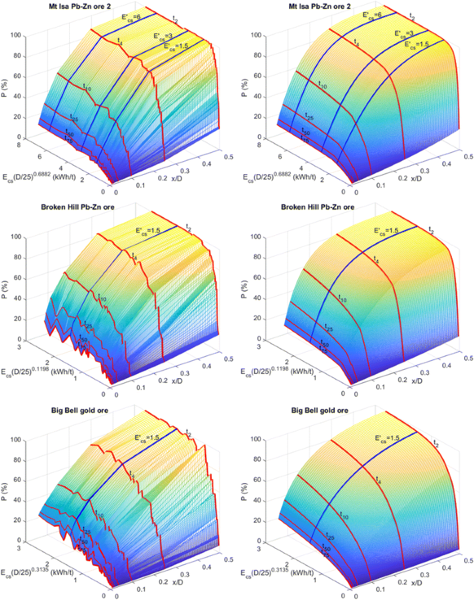
  Breakage surfaces for six of Banini’s (2002) rocks. Left: Banini’s raw data. Right: as predicted from the double fan fits with Eq. 18b, using the parameters in Table 6 ($\lambda$, $E_{{{\text{cs}},0}}^{\prime p}$, $x_{0}^{\prime p}$, $E^{\prime *}$, $E_{{{\text{cs}},0}}^{\prime s}$, $x_{0}^{\prime s}$) and Table 7 ($\alpha_{100}^{p}$, $\alpha_{50}^{p}$, $b^{p}$, $\alpha_{100}^{s}$, $\alpha_{50}^{s}$, $b^{s}$). The lines shown are size distributions for scaled crushing energy of 1.5, 3 and 6 kWh/t (blue lines; 3 and 6 kWh/t ones are absent in Broken Hill and Big Bell plots since the maximum scaled energy is less than 3 kWh/t), and the breakage indexes t₂, t₄, t₁₀, t₂₅, t₅₀ and t₇₅ (red lines). Supplement to Fig. 15

References

Banini GA (2002) An integrated description of rock breakage in comminution machines. PhD thesis, JKMRC, Julius Kruttschnitt Mineral Research Centre, Univ Qld, Indoroopilly QLD
Bourgeois F (1993) Single-particle fracture as a basis for microscale modeling of comminution processes. PhD thesis, Department of Metallurgical Engineering, University of Utah
Bourgeois F (2016) Personal communication by e-mail, March 17
King RP (2012) Modeling and simulation of mineral processing systems, 2nd edn. Soc for Mining, Metallurgy, and Exploration, Inc., Colorado
MATLAB Release 2016b (2016) The MathWorks Inc, Natick
Napier-Munn TJ, Morrell S, Morrison RD, Kojovic T (1996) Mineral comminution circuits: their operation and optimization. JKMRC, Julius Kruttschnitt Mineral Research Centre. Indoroopilly, QLD. ISBN 0 646 28861 x
Narayanan SS (1985) Development of a laboratory single particle breakage technique and its application to ball mill scale-up. PhD thesis, JKMRC, Julius Kruttschnitt Mineral Research Centre, Univ Qld, Indoroopilly QLD. See also next reference
Narayanan SS, Whiten WJ (1988) Determination of comminution characteristics from single particle breakage tests and its application to ball mill scale-up. Trans Inst Min Metall 97:C115–C124
Ouchterlony F (2005) The Swebrec© function, linking fragmentation by blasting and crushing. Min Technol (Trans Inst Min Metal A) 114:A29–A44
Ouchterlony F (2009) Fragmentation characterization; the Swebrec function and its use in blast engineering. In: Sanchidrián JA (ed) Fragblast 9, Proc. 9th Intnl Symp. on Rock Fragmentation by Blasting. Taylor & Francis, London, pp 3–22
Ouchterlony F, Paley N (2013) A reanalysis of fragmentation data from the Red Dog mine—part 2. Blast Fragm 7(3):139–172
Ouchterlony F, Sanchidrián JA, Moser P (2017) Percentile fragment size predictions for blasted rock and the fragmentation–energy fan. Rock Mech Rock Eng 50(4):751–779. https://doi.org/10.1007/s00603-016-1094-x
Rosin P, Rammler E (1933) The laws governing fineness of powdered coal. J Inst Fuel 7:29–36
Sanchidrián JA, Ouchterlony F (2017) A distribution-free description of fragmentation by blasting based on dimensional analysis. Rock Mech Rock Eng 50(4):781–806. https://doi.org/10.1007/s00603-016-1131-9
Sanchidrián JA, Ouchterlony F, Segarra P, Moser P (2014) Size distribution functions for rock fragments. Int J Rock Mech Min Sci 71:381–394
Shi F (2016) A review of the applications of the JK size-dependent breakage model part 1: ore and coal breakage characterization. Int J Miner Process 155:118–129. https://doi.org/10.1016/j.minpro.2016.08.012
Shi F, Kojovic T (2007) Validation of a model for impact breakage incorporating particle size effect. Int J Miner Process 82:156–163
Shi F, Kojovic T, Larbi-Bram S, Manlapig E (2009) Development of a rapid particle breakage characterization device—the JKRBT. Miner Eng 22:602–612
Vogel L, Peukert W (2003) Breakage behaviour of different materials – construction of a mastercurve for the breakage probability. Powder Technol 129:101–110
Weibull W (1939) A statistical theory of the strength of materials. Ingenjörsvetenskapsakademiens handlingar, vol 151. Generalstabens litografiska anstalts förlag, Stockholm
Weibull W (1951) A statistical distribution function of wide applicability. J Appl Mech Trans ASME 18:293–297
Yu P, Xie W, Liu LX, Powell MS (2017) The development of the wide-range 4D appearance function for breakage characterisation in grinding mills. Miner Eng 110:1–11
Acknowledgements
The authors are really grateful to Prof. Peter Moser, vice chancellor of Montanuniversitaet Leoben, for his long-term enthusiastic support of fragmentation research and his long-standing friendship. Thanks also go to Dr Frank Shi, JKMRC, for providing relevant references and for discussing his breakage index equation with the first author. Funding for this work was provided by Montanuniversitaet Leoben and Universidad Politécnica de Madrid. EU Horizon 2020 project Sustainable Low Impact Mining (SLIM), grant agreement No. 730294, has paid the publication costs of this paper. Open access funding provided by Montanuniversität Leoben
Author information
Authors and Affiliations
Corresponding author