On Gromov’s Method of Selecting Heavily Covered Points

Abstract

A result of Boros and Füredi ($d=2$) and of Bárány (arbitrary $d$) asserts that for every $d$ there exists $c_d>0$ such that for every $n$-point set $P\subset {\mathbb {R}}^d$, some point of ${\mathbb {R}}^d$ is covered by at least of the $d$-simplices spanned by the points of $P$. The largest possible value of $c_d$ has been the subject of ongoing research. Recently Gromov improved the existing lower bounds considerably by introducing a new, topological proof method. We provide an exposition of the combinatorial component of Gromov’s approach, in terms accessible to combinatorialists and discrete geometers, and we investigate the limits of his method. In particular, we give tighter bounds on the cofilling profiles for the $(n-1)$-simplex. These bounds yield a minor improvement over Gromov’s lower bounds on $c_d$ for large $d$, but they also show that the room for further improvement through the cofilling profiles alone is quite small. We also prove a slightly better lower bound for $c_3$ by an approach using an additional structure besides the cofilling profiles. We formulate a combinatorial extremal problem whose solution might perhaps lead to a tight lower bound for $c_d$.

1 Introduction

Let $P\subset {\mathbb {R}}^2$ be a set of $n$ points in general position (i.e., no three points collinear). Boros and Füredi [3] showed that there always exists a point $a\in {\mathbb {R}}^2$ contained in a positive fraction of all the $\left( {\begin{array}{c}n\\ 3\end{array}}\right)$ triangles spanned by $P$, namely, in at least $\frac{2}{9}\left( {\begin{array}{c}n\\ 3\end{array}}\right) - O(n^2)$ triangles. (Generally we cannot assume $a\in P$, as the example of points in convex position shows.)

This result was generalized by Bárány [2] to point sets in arbitrary fixed dimension:

Theorem 1

(Bárány [2]) Let $P$ be a set of $n$ points in general position in ${\mathbb {R}}^d$ (i.e., no $d+1$ or fewer of the points are affinely dependent). Then there exists a point in ${\mathbb {R}}^d$ that is contained in at least

$$\begin{aligned} c_d \cdot \big (\begin{array}{c}{n}\\ {d+1}\end{array}\big ) - O(n^d) \end{aligned}$$

$d$-dimensional simplices spanned by the points in $P$, where the constant $c_d>0$ (as well as the constant implicit in the $O$-notation) depend only on $d$.

The largest possible value of $c_d$ has been the subject of ongoing research. With some abuse of notation, we will henceforth denote by $c_d$ the largest possible constant for which Theorem 1 holds true.

Upper Bounds. Bukh, Matoušek and Nivasch [4] showed that¹

$$\begin{aligned} c_d \le \frac{(d+1)!}{(d+1)^{(d+1)}}\sim \frac{\sqrt{2\pi d}}{e^d} = e^{-\Theta (d)} \end{aligned}$$

(1)

by constructing examples of $n$-point sets $P$ in ${\mathbb {R}}^d$ for which no point in ${\mathbb {R}}^d$ is contained more than $(\tfrac{n}{d+1})^{d+1} -O(n^d)$ many $d$-simplices spanned by $P$.

Lower Bounds. The result of Boros and Füredi says that $c_2 \ge 2/9$, which matches the upper bound in (1). For general $d$, Bárány’s proof yields

$$\begin{aligned} c_d \ge \frac{1}{(d+1)^d}, \end{aligned}$$

which is smaller than (1) by a factor of $d!$. In [20], the lower bound was improved by a factor of roughly $d$ to

$$\begin{aligned} c_d \ge \frac{d^2 +1}{(d+1)^{d+1}}, \end{aligned}$$

but this narrowed the huge gap between upper and lower bounds only slightly. Moreover, Bukh, Matoušek and Nivasch showed that the method in [20] cannot be pushed farther. An improvement of the lower bound for $c_3$ by a clever elementary geometric argument was recently achieved by Basit et al. [5].

We refer to [4] for a more detailed discussion of the problem and related results.

Gromov’s Results. Recently, Gromov [9] introduced a new, topological proof method, which improves on the previous lower bounds considerably and which, moreover, applies to a more general setting, described next.

An $n$-point set $P \subseteq {\mathbb {R}}^d$ determines an affine map $T$ from the $(n-1)$-dimensional simplex $\Delta ^{n-1} \subseteq {\mathbb {R}}^{n-1}$ to ${\mathbb {R}}^d$ as follows. Label the vertices of $\Delta ^{n-1}$ by $V=\{v_1,\ldots , v_n\}$, and the points as $P=\{p_1,\ldots , p_n\}$. Then $T$ is given by mapping $v_i$ to $p_i$, $1\le i \le n$, and by interpolating linearly on the faces $\Delta ^{n-1}$.

Thus, Bárány’s result can be restated by saying that for any affine map $T :$ $\Delta ^{n-1} \rightarrow {\mathbb {R}}^d$, there exists a point in ${\mathbb {R}}^d$ that is contained in the $\psi$-images of at least $-O(n^d)$ many $d$-dimensional faces of $\Delta ^{n-1}$.

Gromov shows that, more generally², the following is true:

Theorem 2

([9]) For an arbitrary continuous map $T :\Delta ^{n-1} \rightarrow {\mathbb {R}}^d$, there exists a point in ${\mathbb {R}}^d$ that is contained in the $T$-images of at least many $d$-faces of $\Delta ^{n-1}$, where $c^{\mathrm{top}}_d>0$ is a constant that depends only on $d$.

By the same abuse of notation as before, $c^{\mathrm{top}}_d$ will also henceforth denote the largest constant for which Theorem 2 holds. In particular, $c_d \ge c^{\mathrm{top}}_d$.

Gromov’s method gives

$$\begin{aligned} c_d \ge c^{\mathrm{top}}_d \ge \frac{2d}{(d+1)! (d+1)}. \end{aligned}$$

(2)

For $d=2$, this yields the tight bound $c^{\mathrm{top}}_2 = c_2 =2/9$. For general $d$, Gromov’s result improves on the earlier bounds by a factor exponential in $d$, but it is still of order $\mathrm{{e}}^{-\Theta (d\log d)}$ and thus far from the upper bound.

One of the goals of this paper is to provide an exposition of the combinatorial component of Gromov’s approach, in terms accessible to combinatorialists and discrete geometers.

After a preliminary version of this paper was written and circulated, Karasev [12] found a very short and elegant proof of Gromov’s bound (2) for affine maps.

Karasev’s proof, which he himself describes as a “decoded and refined” version of Gromov’s proof, combines probabilistic and topological arguments, but he avoids the heavy topological machinery applied in Gromov’s proof and only uses the elementary notion of the degree of a piecewise smooth map between spheres.

Karasev’s argument can be modified and extended so that it covers the case of arbitrary continuous maps into ${\mathbb {R}}^d$ (but not yet into general $d$-dimensional manifolds). Furthermore, the combinatorial and the topological aspects of the argument, which are intertwined in Karasev’s proof, can be split into two independent parts. In this way, any combinatorial improvement on the cofilling profiles or on the pagoda problem introduced in Sect. 6 immediately implies improved bounds for Theorem 2 also via this simpler topological route. We plan to discuss this in more detail in a separate note.

Coboundaries and Cofilling Profiles. We need two basic notions, coboundaries and cofilling profiles, which have their roots in cohomology but which can be defined in elementary and purely combinatorial terms.

Let $V$ be a fixed set of $n$ elements, w.l.o.g., $V=[n]:=\{1,2,\ldots , n\}$. We will always assume that $n$ is sufficiently large.

In topological terms, we think of the $(n-1)$-dimensional simplex $\Delta ^{n-1}$ as a combinatorial object (an abstract simplicial complex), namely, as the system of all subsets of $V$. Thus, given a subset $f \subseteq V$, we will also sometimes refer to $f$ as a face of $\Delta ^{n-1}$, and the dimension of a face is defined as $\dim f:= |f|-1$.

Let $E\subseteq {{V}\atopwithdelims (){d}}$ be a system of (unordered) $d$-tuples, or in other words, of $(d-1)$-dimensional faces.

We write $\Vert E\Vert := |E|/{n\atopwithdelims ()d}$ for the density (normalized support size) of $E$; one can also interpret $\Vert E\Vert$ as the probability that a random $d$-tuple lies in $E$. The notation $\Vert E\Vert$ implicitly refers to $d$ and $n$, which have to be understood from the context.

The coboundary $\delta E$ is the system of those $(d+1)$-tuples $f\in {V\atopwithdelims ()d+1}$ that contain an odd number of $e\in E$. (For $d=2$, this notion and some of the following considerations are related to Seidel switching and two-graphs, which are notions studied in combinatorics—see the end of Sect. 2 for an explanation and references.)

We emphasize that $\delta E$ also depends on the ground set $V$, and sometimes we may write $\delta _V E$ instead of $\delta E$ to avoid ambiguities.

Many different $E$’s may have the same coboundary. We call $E$ minimal if $\Vert E\Vert \le \Vert E'\Vert$ for every $E'$ with $\delta E'=\delta E$.

We define the cofilling profile ³ as follows:

$$\begin{aligned} \varphi _d(\alpha ):=\liminf _{|V|=n\rightarrow \infty }\min \big \{\Vert \delta E\Vert : E\subseteq {\textstyle \left( {\begin{array}{c}V\\ d\end{array}}\right) } \text{ minimal }, \Vert E\Vert \ge \alpha \big \}. \end{aligned}$$

Equivalently, one can also view this notion as follows. Suppose we are given a system $F \subseteq \left( {\begin{array}{c}V\\ d+1\end{array}}\right)$, and we are guaranteed that $F$ is a coboundary, i.e., that $F=\delta E$ for some $E$. Now we want to know the smallest possible density $\Vert E\Vert$ of an $E$ with $F=\delta E$, as a function of $\Vert F\Vert$. It suffices to consider minimal $E$’s, and $\varphi (\alpha ) \ge \beta$ means that if we are forced to take $\Vert E\Vert \ge \alpha$, then we must have $\Vert F\Vert \ge \beta$.

We also remark that there is no minimal $E$ with $\Vert E\Vert > 1/2$ (see Sect. 2), so formally, $\varphi _d(\alpha )=\infty$ for $\alpha >1/2$ (since we take the minimum over an empty set).

As a warm-up, let us consider case $d=1$: In this case, we can view an $S\subseteq \left( {\begin{array}{c}V\\ 1\end{array}}\right)$ simply as a subset of $S\subseteq V$, and $\delta S$ is the set of edges of the complete bipartite graph with color classes $S$ and $V\setminus S$; in graph theory, one also speaks of the edge cut determined by $S$ in the complete graph on $V$.

The minimality of $S$ simply means that $|S| \le n/2$. It follows that $\varphi _1(\alpha )=2\alpha (1-\alpha )$, $0\le \alpha \le \frac{1}{2}$.

For general $d$, the following basic bound for $\varphi _d$ was observed by Gromov, and independently by Linial, Meshulam, and Wallach [15, 17] (and maybe by others). In our terminology, it can be stated as follows:

Lemma 3

(Basic Cofilling Bound) For every $d\ge 1$ and all $\alpha \in [0,1]$,

$$\begin{aligned} \varphi _d(\alpha )\ge \alpha . \end{aligned}$$

We will recall a simple combinatorial proof of this bound, along with other basic properties of the coboundary operator, in Sect. 2. A simple example shows that the basic bound is attained with equality for $\alpha =\tfrac{(d+1)!}{(d+1)^{(d+1)}}\approx e^{-(d+1)}$, but for smaller $\alpha$, improvements are possible, as we will discuss later.

In Sect. 3, we present an outline of topological part of Gromov’s argument, which yields the following general lower bound.

Proposition 4

([9]) For every $d\ge 1$,

$$\begin{aligned} c^{\mathrm{top}}_d\ge \varphi _{d}\big (\tfrac{1}{2} \varphi _{d-1}\big (\tfrac{1}{3} \varphi _{d-2}\big (\ldots \tfrac{1}{d} \varphi _1\big (\tfrac{1}{d+1}\big )\ldots \big )\big )\big ). \end{aligned}$$

Theorem 2 follows from this proposition by using $\varphi _1(\alpha )=2\alpha (1-\alpha )$ and the basic bound for all $d\ge 2$.

Better bounds on the $c^{\mathrm{top}}_d$ would immediately follow from Proposition 4 if one could improve on the basic cofilling bound in an appropriate range of $\alpha$’s; this is a purely combinatorial question (and a quite nice one, in our opinion).

We establish the following lower bounds for $\varphi _2$ and $\varphi _3$:

Theorem 5

For $d=2$ and all $\alpha \le \frac{1}{4}$, we have the lower bound

$$\begin{aligned} \varphi _2(\alpha ) \ge \tfrac{3}{4}\big (1-\sqrt{1-4\alpha }\big )(1-4\alpha )= \tfrac{3}{2}\alpha -\tfrac{9}{2}\alpha ^2-3\alpha ^3-O(\alpha ^4). \end{aligned}$$

Figure 1 shows a plot of this lower bound.

Fig. 1

The lower and upper bounds on $\varphi _2(\alpha )$: the straight line is the basic bound, the top one the upper bound (Proposition 7), and the bottom (most curved) is the lower bound (Theorem 5)

Theorem 6

For $d=3$ and $\alpha$ sufficiently small,

$$\begin{aligned} \varphi _3(\alpha )\ge \tfrac{4}{3}\alpha - O(\alpha ^2) \end{aligned}$$

(with a constant that could be made explicit).

These theorems will be proved in Sects. 4 and 5, respectively.

They do not improve on Gromov’s lower bounds for $c_3$, for example, since they do not beat the basic bound for the values of $\alpha$ needed in Proposition 4 for $d$ small. However, they do apply if we take $d$ sufficiently large in Proposition 4, and so they at least show that Gromov’s lower bound on $c^{\mathrm{top}}_d$ is not tight for large $d$.

After the research reported in this paper was completed, Král’ et al. [13] proved the lower bound $\varphi _2(\alpha )\ge \frac{9}{7}\alpha (1-\alpha )$. This is better than the bound of Theorem 5 for $\alpha$ larger than approximately $0.0626$, and it does improve on Gromov’s lower bound for $c_3$.

The bounds in Theorems 5 and 6 may look like only minor improvements over the basic bound, but it turns out that they have the right order of magnitude for $\alpha$ tending to $0$. Indeed, we have the following upper bound on the $\varphi _d$’s.

Proposition 7

For all $d\ge 1$ and $\alpha \le \frac{1}{d+1}$, let $\sigma \in [0,1)$ be the smallest positive number with $\alpha =d!\sigma (\frac{1-\sigma }{d})^{d-1}$. Then

$$\begin{aligned} \varphi _d(\alpha ) \le \tfrac{d+1}{d}\alpha (1-\sigma ), \end{aligned}$$

and consequently, $\varphi _d(\alpha )\le \frac{d+1}{d}\alpha$.

These bounds are plotted in Fig. 2.

Fig. 2

Plots of the upper bounds from Proposition 7 for $d=2,3,4$, together with the basic bound.

Proposition 7 follows from a simple example, whose special case with $\alpha =\frac{1}{d+1}$ has already been noted in [9] and in [15, 17]. We present the example and its analysis in Sect. 2.

We conjecture that the bound in Proposition 7 is the truth, and moreover, that the example mentioned above is essentially the only possible extremal example. However, a proof may be challenging even for the $d=2$ case. On the other hand, we believe that a suitable extension of the proof of Theorem 6 may provide a bound of the form $\varphi _d(\alpha )\ge \frac{d+1}{d}\alpha -o(\alpha )$ as $\alpha \rightarrow 0$. At present it seems that such an extension would be highly technical and complicated.

In view of the upper bound $\varphi _d(\alpha )\le \frac{d+1}{d}\alpha$, Gromov’s lower bound on $c_d$ cannot be improved by more than a factor of roughly $d$ using Proposition 4 alone.

In Sect. 6, we introduce a somewhat different approach, which goes beyond Proposition 4 and uses additional combinatorial structure, and we show that it can provide a slightly better lower bound for $c_3$. We formulate a combinatorial extremal problem whose solution might perhaps lead to a tight lower bound for the $c^{\mathrm{top}}_d$.

2 Basics

Linearity of the Coboundary. For systems $E,E' \subseteq \left( {\begin{array}{c}V\\ d\end{array}}\right)$ of $d$-tuples, $E+E'$ means the symmetric difference.

The coboundary operator is (well known and easily checked to be) linear with respect to this operation, i.e.,

$$\begin{aligned} \delta (E+E')=\delta E+\delta E', \end{aligned}$$

and we have

$$\begin{aligned} \delta \delta E=0, \end{aligned}$$

where $0$ means the empty system of $(d+2)$-tuples.

Cochains, Coboundaries, and Cocycles. A system $E\subseteq \left( {\begin{array}{c}V\\ d\end{array}}\right)$ of $d$-tuples is also sometimes called a $(d-1)$-dimensional cochain,⁴ or simply $(d-1)$-cochain. Later on, when working with systems of tuples of various arities, it will be convenient to use this terminology. A cochain $E$ is called a cocycle if $\delta E=0$, and it is a coboundary if it can be written as $E=\delta D$ for some $(d-2)$-chain $D$.

In algebraic terms, a $(d-1)$-cochain $E\subseteq \left( {\begin{array}{c}V\\ d\end{array}}\right)$ can be identified with a $0/1$-vector indexed by the elements of $\left( {\begin{array}{c}V\\ d\end{array}}\right)$, which we can interpret as an element of the vector space ${\mathbb {Z}}_2^{\left( {\begin{array}{c}V\\ d\end{array}}\right) }$ over the $2$-element field ${\mathbb {Z}}_2$, and the symmetric difference $+$ corresponds to the usual addition is this vector space. The coboundary operators are linear maps between these spaces (mapping $(d-1)$-cochains to $d$-cochains). The $(d-1)$-cocycles are precisely the elements of the kernel of this linear map, and the $d$-coboundaries are the elements of the image. The property $\delta \delta =0$ is usually called the chain complex property.

Minimality. As we have seen, every coboundary is also a cocycle, i.e., if $F=\delta E \subseteq \left( {\begin{array}{c}V\\ d+1\end{array}}\right)$, then $\delta F=0$.

In our setting, this is a complete characterization, i.e., $F \subseteq \left( {\begin{array}{c}V\\ d+1\end{array}}\right)$ is a coboundary if and only if $\delta F=0$. Topologically speaking, this is because the $(n-1)$-simplex has zero cohomology.

We stress that there is one exceptional case, namely, $d=0$. There are two $0$-cocycles $F\subseteq \left( {\begin{array}{c}V\\ 1\end{array}}\right)$, namely, $F=V$, the set of all vertices, and $F=0$, the empty set of vertices. However, by definition, $0$ is considered to be a coboundary, but $V$ is not. In topological terms, this is because we are working with ordinary, non-reduced cohomology.⁵ This will be formally important in Sect. 3.1.

Because of the equivalence of cocycles and coboundaries, for $d-1 \ge 1$, minimality of $E$ can be equivalently characterized as follows: $E$ is minimal if $\Vert E\Vert \le \Vert E+\delta D\Vert$ for every $D\subseteq {V\atopwithdelims ()d-1}$. Thus, minimality means that $E$ contains at most half of the $d$-tuples from each system of the form $\delta D$. Consequently, if $E$ is minimal and $E'\subseteq E$, then $E'$ is minimal as well.

It also follows from the alternative characterization of minimality that every minimal $E$ satisfies $\Vert E\Vert \le 1/2$. To see this, let $D=\{x\}$ be a singleton set consisting of a single $(d-1)$-tuple $x$. Then $|E \cap \delta D| \le 1/2 | \delta D|$ means that $x$ is incident to at most $|\delta D|/2=\frac{n-d+1}{2}$ many $d$-tuples $e \in E$. Summing up over all $x \in \left( {\begin{array}{c}V\\ d-1\end{array}}\right)$, we get $d |E| \le \left( {\begin{array}{c}n\\ d-1\end{array}}\right) (n-d+1)/2$, and hence $|E| \le \left( {\begin{array}{c}n\\ d\end{array}}\right) /2$.

As was remarked above, minimality refers to a fixed vertex set $V$. If a minimal $E \subseteq \left( {\begin{array}{c}V\\ d\end{array}}\right)$ happens to be contained in $\left( {\begin{array}{c}W\\ d\end{array}}\right)$ for some subset $W\subset V$ then, considered as a set of subsets of $W$, it needs no longer be minimal. For example, suppose we partition $V$ into three vertex sets $V_1, V_2, V_3$ of size $n/3$ each and let $E=\{ \{v_1,v_2\}: v_1\in V_1, v_2 \in V_2\}$, the (edge set of the) complete bipartite graph between $V_1$ and $V_2$. Then it is not hard to check that $E$ is minimal as a subset of $\left( {\begin{array}{c}V\\ 2\end{array}}\right)$, but not as a subset of $\left( {\begin{array}{c}V_1 \cup V_2\\ 2\end{array}}\right)$.

Links of Vertices. For system $E\subseteq \left( {\begin{array}{c}V\\ d\end{array}}\right)$ of $d$-tuples and a vertex $v\in V$, let us write $E_v:=\{e\in E: v\in e\}$. The link of $v$ in $E$ is the system of $(d-1)$-tuples $\mathop {\mathrm{lk}}\nolimits (v,E):=\{e\setminus \{v\}: e\in E_v\}$.

It is easy to check the following formula for the coboundary of the link:

$$\begin{aligned} \delta \mathop {\mathrm{lk}}\nolimits (v,E) = E_v + \mathop {\mathrm{lk}}\nolimits (v,\delta E_v) \end{aligned}$$

(3)

(the $+$ on the right-hand side is actually a disjoint union in this case).

The Basic Bound for the Filling Profile. We now recall a combinatorial proof of the basic lower bound for $\varphi _d$.

Proof of Lemma 3

Let $F\subseteq {V\atopwithdelims ()d+1}$ be a coboundary, and let $\beta :=\Vert F\Vert$. We will show that there exists an $E\in \left( {\begin{array}{c}V\\ d\end{array}}\right)$ with $\delta E=F$ and $\big \Vert E\big \Vert \le \beta$. It follows, in particular, that any minimal $E'$ with $\delta E'= F$ satisfies $\big \Vert E'\big \Vert \le \beta$, which proves the lemma.

We define the normalized degree of $v \in V$ as $\Vert \mathop {\mathrm{lk}}\nolimits (v,F)\Vert =|\mathop {\mathrm{lk}}\nolimits (v,F)|/{n\atopwithdelims ()d}$.

A simple counting argument shows that the average normalized degree of a vertex equals $\beta =\big \Vert F\big \Vert$. In particular, there exists a vertex $v$ of normalized degree at most $\beta$; so we fix such a vertex $v$ and set $E:=\mathop {\mathrm{lk}}\nolimits (v,F)$. We will check that $\delta E=F$.

Let $F_{\setminus v}:=F\setminus F_v$. Since $F$ is a coboundary, we have $\delta F=0$, and thus $\delta F_v=\delta F_{\setminus v}$.

Let us consider an arbitrary $(d+1)$-tuple $f$ and distinguish two cases.

Case 1. If $v\in f$, then it is easily seen that $f\in \delta E$ is equivalent to $f\in F$.

Case 2. Next, assume $v\not \in f$. By definition of $E$, $d$-tuples $e\in E$ are in one-to-one correspondence with the $(d+1)$-tuples $e\cup \{v\}\in F_v$. It follows that, $f\in \delta E$ iff $f^+:=f\cup \{v\}\in \delta F_v$. This in turn is the case iff $f^+\in \delta F_{\setminus v}$ because $\delta F_v=\delta F_{\setminus v}$. Since the sets of $F_{\setminus v}$ avoid $v$, only one $(d+1)$-tuple of $F_{\setminus v}$ may be contained in $f^+$, namely $f$. Thus, $f^+\in \delta F_{\setminus v}$ iff $f\in F_{\setminus }$ iff $f\in F$ (since we assume $v\not \in f$). Hence, $f\in \delta E$ iff $f\in F$ also in this case.$\square$

The Upper Bound Example. Here we prove Proposition 7, the upper bound on the cofilling profile $\varphi _d$.

Let $\sigma \in [0,1]$ be a parameter. We partition the vertex set $V$ into $V_1,\ldots ,V_{d+1}$, where $|V_1|=\sigma n$ and the remaining vertices are divided evenly, i.e., $|V_i|= \frac{1-\sigma }{d} n$, $i>1$ (we ignore divisibility issues). Let $E$ consist of all $d$-tuples that use exactly one point from each of $V_1,\ldots ,V_d$; see Fig. 3. We have $\Vert E\Vert =:\alpha =d!\sigma (\frac{1-\sigma }{d})^{d-1}$.

Fig. 3

The upper bound example in the case $d=3$. The solid triangle depicts a typical element of $E$, and the dashed segments complete it to a tetrahedron that is a typical element of $\delta E$

Then $F:=\delta E$ is the complete $(d+1)$-partite system on $V_1,\ldots ,V_{d+1}$, and $\Vert \delta E\Vert =\frac{d+1}{d}\alpha (1-\sigma )$. For a suitable choice of $\sigma$, this matches the quantitative bounds in Proposition 7, and it remains to check the minimality of $E$, which is easy (and stated by Gromov and by Meshulam et al. without proof): Let us consider some $E'$ with $F=\delta E'$. Every $f\in F$ contains at least one $e\in E'$, while every $e\in E'$ is contained in at most $M:=\max _i{|V_i|}$ many $f\in F$. So $|E'|\ge |F|/M=|E|$. $\square$

On Seidel’s Switching. In combinatorics, a two-graph (see the references below) is a set $F\subseteq {V\atopwithdelims ()3}$ of triples with $\delta F=0$, i.e., a cocycle in our terminology). As we have mentioned, this is equivalent to $F$ being a coboundary, i.e., to the existence of some $E\subseteq {V\atopwithdelims ()2}$ with $F=\delta E$. The system of all possible $E'$ with $\delta E'=F$ is called the Seidel switching class of $E$.

Two-graphs and Seidel’s switching were introduced by Van Lint and Seidel [19] and further studied by many authors, because of their connections with equiangular lines, strongly regular graphs, and interesting finite groups, for example (for surveys see, e.g., Seidel and Taylor [18] or Hage [10]).

Numerous authors investigated the computational complexity of various problems related to Seidel’s switching (we refer to [11, 14] for citations). For us, the following result is of particular interest: It is NP-complete to decide if a given $E\subseteq {V\atopwithdelims ()2}$ is minimal (in its Seidel switching class), as was proved by Jelínková [11]. Her reduction produces only $E$’s with $\Vert E\Vert \ge \frac{1}{2}$ and $\Vert E'\Vert \ge \frac{1}{4}$ for all $E'$ in the same switching class; however, recently Jelínek (private communication, September 2010) was able to modify the reduction, showing that the problem remains NP-complete even if we restrict only to $E$’s with $\Vert E\Vert \le c$, for every fixed $c>0$. This shows that minimal sets have a complicated structure, and one cannot expect to find a reasonable characterization.

3 An Outline of Gromov’s Topological Approach

In this section, we give a rather informal and elementary outline of the topological part of Gromov’s approach (Sects. 2.2, 2.4, 2.5, and 2.6 of [9]). This outline is not directly related to the new (combinatorial) results of the present paper.

We strive to keep the discussion as elementary as possible for as long as possible. For this reason, we restrict ourselves to the most basic (affine) setting of finite set $P$ of $n$ points in general position in ${\mathbb {R}}^d$, which allows us to describe most steps in the argument in simple geometric terms.

As remarked above, Gromov’s method applies in much more general situations. In Sect. 3.5, we briefly discuss the more general setting and also include some remarks as to how our elementary discussion would be formulated in more standard topological terms.

We begin with an outline of our outline, by means of an example.

Example 8

Let $P=\{p_1,\ldots , p_5\}$ be the set of five points in ${\mathbb {R}}^2$ depicted by bold dots in Fig. 4, and let $V=[5]:=\{1,2,3,4,5\}$.

Consider the three points $x,y,z$ marked by crosses in the picture. These three points are in general position w.r.t. $P$, in the sense that they do not lie on any line segment spanned by $P$, and no point of $P$ lies on any of the line segments spanned by $x,y,z$.

Let $F_x=\{ \{1,2,3\}, \{1,2,4\}, \{1,2,5\}\}$ be the set of all triples $\{i,j,k\} \in \left( {\begin{array}{c}V\\ 3\end{array}}\right)$ such that $x$ lies in the triangle $p_i p_j p_k$, and let $F_y=\{\{1,2,3\},\{2,3,4\},\{2,3,5\}\}$ and $F_z=\{\{1,2,3\}, \{1,3,5\},$ $\{2,3,4\},\{3,4,5\}\}$ be defined analogously as the (index sets of) triangles containing $y$ and $z$, respectively.

Let $F_{xy}=\{ \{2,4\}, \{2,5\}\}$ be the set of pairs $\{i,j\} \in \left( {\begin{array}{c}V\\ 2\end{array}}\right)$ such that the line segment $p_i p_j$ intersects the line segment $xy$, and let $F_{yz}=\{\{3,5\}\}$ and $F_{xz}=\{ \{1,5\}, \{2,4\}, \{4,5\}\}$ be defined analogously.

Finally, let $F_{xyz}= \{5\}$ be the set of indices $i \in V$ such that $p_i$ lies in the triangle $xyz$ (here, we identify elements $i \in V$ with singleton sets $\{i\} \subseteq V$ to simplify notation).

The basic observation is that these sets satisfy the relations

$$\begin{aligned}&\delta F_x = \delta F_y = \delta F_z =0,\\&F_x + F_y = \delta F_{xy},\quad F_y + F_z =\delta F_{yz}, \quad F_x+ F_z =\delta F_{xz}, \end{aligned}$$

and

$$\begin{aligned} F_{xy} + F_{yz} + F_{xz} = \delta F_{xyz}. \end{aligned}$$

It is straightforward to verify this in the specific example at hand, but it may in fact be easier—and an instructive exercise—to check that these relations are not a coincidence, but hold in general for any finite set $P \subseteq {\mathbb {R}}^2$ and any triple of points $x,y,z$, assuming only general position. Moreover, similar facts hold in ${\mathbb {R}}^d$. We discuss a proof of the general case below.

Fig. 4

A set of five labeled points in general position in ${\mathbb {R}}^2$ (the image of $\Delta ^4$ under an affine map)

Informally speaking and in very general terms, the structure of Gromov’s topological approach can be summarized as follows. Each step of the argument will be discussed in more detail in a separate subsection below. We fix $d\ge 1$ (the target dimension) and $V=[n]$ (the vertex set of the $(n-1)$-simplex $\Delta ^{n-1}$).

• 1. We define a topological space $\mathcal {Z}^d=\mathcal {Z}^d(\Delta ^{n-1})$, the space of $d$-dimensional cocycles (of the $(n-1)$-simplex).

  This space is a simplicial set, i.e., a space built of vertices, edges, triangles, and higher-dimensional simplices like a simplicial complex, but simplices are allowed to be glued to each other and to themselves in more general ways (in a first approximation, simplicial sets can be thought of as higher-dimensional analogues of multigraphs with loops, while simplicial complexes are higher-dimensional analogues of simple graphs).

  The vertices of $\mathcal {Z}^d$ are the $d$-dimensional cocycles $F\subseteq \left( {\begin{array}{c}V\\ d+1\end{array}}\right)$. The edges of $\mathcal {Z}^d$ correspond to relations of the form $F_1 + F_2 = \delta F_{12}$, where $F_{12}\subseteq \left( {\begin{array}{c}V\\ d\end{array}}\right)$. The triangles of $\mathcal {Z}^d$ correspond to a triple of $d$-dimensional cocycles $F_1$, $F_2$, $F_3$, edges between them, and a relation of the form $F_{12} + F_{23} + F_{31} = \delta F_{123}$, where $F_{123} \subseteq \left( {\begin{array}{c}V\\ d-1\end{array}}\right)$, etc.

  We stress that $\mathcal {Z}^d$ depends only on $n$ and $d$ and is defined purely combinatorially. Moreover, as a combinatorial object, it is huge. For instance, the number of vertices of $\mathcal {Z}^d$ ($d$-dimensional cocycles of the simplex) is $2^{\left( {\begin{array}{c}n-d\\ d\end{array}}\right) }$.

• 2. With every labeled $n$-point set $P\subseteq {\mathbb {R}}^d$, we associate a particular subspace⁶ $\mathcal {W} =\mathcal {W}(P) \subseteq \mathcal {Z}^d$.

  A concrete way of doing this is to choose a triangulation $\mathcal {T}$ of ${\mathbb {R}}^d$ that is in general position w.r.t. $P$ (i.e., no $k$-dimensional simplex of $\mathcal {T}$ intersects any $\ell$-dimensional simplex spanned by $P$ if $k+\ell < d$). With every vertex $x$ of $\mathcal {T}$ we associate the set

  $$\begin{aligned} F_x:=\big \{ f=\{i_0,i_1,\ldots , i_d\} \in \textstyle {\left( {\begin{array}{c}V\\ d+1\end{array}}\right) }: x \in p_{i_0} p_{i_1}\cdots p_{i_d}\big \} \end{aligned}$$

  of (indices of) $d$-simplices spanned by $P$ that contain $x$. As indicated by the example, each such $F_x$ is a cocycle, i.e., a vertex of $\mathcal {Z}^d$ (but not all vertices of $\mathcal {Z}^d$ may be of this special form).

  With every edge $xy$ of $\mathcal {T}$, we associate the set $F_{xy}$ of $d$-tuples from $V$ such that the corresponding points of $P$ span a $(d-1)$-simplex that intersects $xy$. As in the example, we get the relation $F_x + F_y =\delta F_{xy}$, and hence an edge of $\mathcal {Z}^d$.

  Similarly, each $k$-dimensional simplex of the triangulation gives rise to a $k$-simplex of $\mathcal {Z}^d$ (but not all $k$-simplices in $\mathcal {Z}^d$ may be of this form). We define the subspace $\mathcal {W}$ to consist of all simplices of $\mathcal {Z}^d$ that are obtained from an odd number of simplices of $\mathcal {T}$ using this construction. (In principle, different simplices of the triangulation $\mathcal {T}$ may yield the same $k$-simplex in $\mathcal {Z}^d$.)

• 3. It follows from a theorem in algebraic topology, the Almgren–Dold–Thom Theorem, that the subspace $\mathcal {W}$ is not contractible inside $\mathcal {Z}^d$.

• 4. If we choose the triangulation $\mathcal {T}$ sufficiently finely, then for every point $a\in {\mathbb {R}}^d$, there is a vertex $x$ of $\mathcal {T}$ with $F_a = F_x$. Thus, if no point of ${\mathbb {R}}^d$ is covered by “many” $d$-simplices of $P$, then all sets $F_x$ are “small.” If this is so, then by purely combinatorial means, we can define a concrete way of contracting the subspace $\mathcal {W}$ to a single point inside $\mathcal {Z}^d$; see Fig. 5. This is a contradiction. Thus, some point must be covered by many $d$-simplices.

Fig. 5

A schematic illustration of the last two steps of the argument: $\mathcal {W}$ is not contractible inside $\mathcal {Z}^d$, but if no point in ${\mathbb {R}}^d$ were covered by sufficiently many $d$-simplices of $P$, then we could contract $\mathcal {W}$ inside $\mathcal {Z}^d$ to a single point

We now proceed to discuss the above steps in more detail.

3.1 Simplicial Sets and the Space of Cocycles

Simplicial sets ⁷ are a generalization of simplicial complexes. As in the case of a simplicial complex, a simplicial set is built from $0$-simplices (vertices), $1$-simplices (edges), $2$-simplices (triangles), and higher-dimensional simplices.

One starts with the vertices, then glues each edge to one or two vertices by its endpoints, then one attaches triangles to vertices or edges along their boundaries, etc. In contrast to simplicial complexes, the attaching may involve various identifications. For instance, both endpoints of an edge may be attached to the same vertex, and two or more $i$-simplices in a simplicial set may have the same boundary. In this respect, simplicial sets can be thought of, in a first approximation, as higher-dimensional analogues of multigraphs with loops. On the other hand, in contrast to general cell complexes, there are restrictions as to what kind of attaching maps are allowed,⁸ which makes simplicial sets more combinatorial than general cell complexes. We refer the reader to the article by Friedman [8] for a very clear and accessible introduction to simplicial sets and to the book by May [16] for a detailed treatment (further references can be found in Friedman’s article).

The key object in Gromov’s method is the space of $d$ -dimensional cocycles, which we denote⁹ by $\mathcal {Z}^d=\mathcal {Z}^d(\Delta ^{n-1})$ and which is a simplicial set defined as follows.

The vertices of $\mathcal {Z}^d$ are the $d$-dimensional cocycles (of the simplex $\Delta ^{n-1}$), i.e., subsets $F\subseteq \left( {\begin{array}{c}V\\ d+1\end{array}}\right)$ such that $\delta F=0$.

The edges of $\mathcal {Z}^d$ are given by two (not necessarily distinct) $d$-cocycles $F_1$ and $F_2$ and a set $F_{12}\subseteq \left( {\begin{array}{c}V\\ d\end{array}}\right)$ such that $\delta F_{12}=F_1+F_2$. We stress that $F_{12}$ and at least one of the $F_i$ are necessary in order to uniquely define an edge in $\mathcal {Z}^d$. If there is a $F_{12}'$ with $\delta F_{12}'=F_1+F_2$ then it defines a different edge of $\mathcal {Z}^d$ connecting the same pair of vertices. On the other hand, if $F_1'$ and $F_2'$ are another pair of $d$-cocycles with $\delta F_{12} =F_1'+F_2'$, then the same $F_{12}$ yields a different edge of $\mathcal {Z}^d$ connecting a different pair of vertices.

In the next step, a triangle of $\mathcal {Z}^d$ is given by a triple of $d$-cocycles $F_1$, $F_2$, $F_3$, a triple of sets $F_{ij}\subseteq \left( {\begin{array}{c}V\\ d\end{array}}\right)$ and a set $F_{123} \subseteq \left( {\begin{array}{c}V\\ d-1\end{array}}\right)$ such that

• (i) $\delta F_{ij}= F_i + F_j$, $1\le i < j \le 3$, and

• (ii) $\delta F_{123} = F_{12}+ F_{13} + F_{23}$.

The $F_i$ and the $F_{ij}$ define three (not necessarily distinct) vertices and three (not necessarily distinct) edges of $\mathcal {Z}^d$ that form the boundary of a triangle, and together with this other data, $F_{123}$ defines a triangle glued in along that boundary. Again, there may be other $F_{123}'$ with the same coboundary, which define different triangles glued to the same boundary (a higher-dimensional analogue of a multiedge), and there may be a different set of $F_i'$ and/or $F_{ij}'$ which also satisfy conditions (i) and (ii); if so, they yield, together with $F_{123}$, a different triangle of $\mathcal {Z}^d$, glued to a different boundary.

One can continue this definition inductively¹⁰ for simplices of arbitrary dimension $r$. The case of $(d+1)$-simplices in $\mathcal {Z}^d$, deserves special attention, however (due to the exceptional behavior of the coboundary operator in dimension zero, i.e., the fact that $V$ is not considered a coboundary, which was mentioned in Sect. 2). A $\big (d+1\big )$-simplex in $\mathcal {Z}^d$ is given by the following data (see Fig. 6): for each $0\le i\le d$ and each $A\in \left( {\begin{array}{c}[d+2]\\ i+1\end{array}}\right)$, there is a set $F_A \in \left( {\begin{array}{c}V\\ d+1-i\end{array}}\right)$ (i.e., a set of $(d-i)$-dimensional faces) such that

$$\begin{aligned} \delta F_A =F_{\partial A}:=\textstyle \sum \limits _{B \in \partial A} F_B \end{aligned}$$

and

$$\begin{aligned} \textstyle \sum \limits _{A \in \left( {\begin{array}{c}[d+2]\\ d+1\end{array}}\right) } F_A=0. \end{aligned}$$

Here, by definition, $\partial A:=\{A\setminus \{a\}:a\in A\}$, called the boundary of $A$.

Fig. 6

An illustration of a $3$-dimensional simplex in $\mathcal {Z}^d$. It is given by four $2$-dimensional cocycles $F_i \in \left( {\begin{array}{c}V\\ 3\end{array}}\right)$, six sets $F_{ij} \in \left( {\begin{array}{c}V\\ 2\end{array}}\right)$, and four sets $F_{ijk} \in \left( {\begin{array}{c}V\\ 1\end{array}}\right)$ (with pairwise distinct indices $i,j,k$ running between $1$ and $4$) that satisfy the relations $\delta F_{ij}= F_i + F_j$, $\delta F_{ijk}=F_{ij}+F_{jk}+F_{ik}$, and $\sum \nolimits _{ijk} F_{ijk}=0$

3.2 Intersections and Cocycles

Let $P =\{p_1,p_2,\ldots , p_n\} \subseteq {\mathbb {R}}^d$ be a labeled set of $n$ points in general position. We think of $V=[n]$ as the set of “labels” of $P$. The goal of this section is to define the subspace $\mathcal {W}=\mathcal {W}(P) \subseteq \mathcal {Z}^d$ for this set $P$.

Let $A=a_0a_1\ldots a_k$ be a $k$-dimensional simplex in ${\mathbb {R}}^d$ that is in general position w.r.t. $P$, i.e., no $i$-face of $A$ intersects any $(d-i-1)$-simplex spanned by $P$, $0\le i \le k$. We define

$$\begin{aligned} F_A:= \big \{\{i_0, i_{1}\ldots , i_{d-k} \} \in {\textstyle \left( {\begin{array}{c}V\\ d+1-k\end{array}}\right) }: A \cap p_{i_0}p_{i_1}\ldots p_{i_{d-k}} \ne \emptyset \big \}. \end{aligned}$$

That is, we consider the $(d-k)$-simplices spanned by $P$ that are intersected by $A$. Each such simplex is of the form $p_{i_0}p_{i_1}\ldots p_{i_{d-k}}$ for some $(d+1-k)$-tuple $\{i_0, i_1 \ldots , i_{d-k} \} \in {\textstyle \left( {\begin{array}{c}V\\ d+1-k\end{array}}\right) }$ of labels, and $F_A$ consists precisely of these tuples. For simplicity, we will also say that $F_A$ corresponds to the set of $(d-k)$-simplices of $P$ intersected by $A$.

Thus, for a point $x \in {\mathbb {R}}^d$ in general position w.r.t. $P$, $F_x =\{ \{i_0,i_1,\ldots , i_d\} \in \left( {\begin{array}{c}V\\ d+1\end{array}}\right) : x \in p_{i_0}p_{i_1}\ldots p_{i_d}\}$ corresponds to the set of $d$-simplices of $P$ that contain $x$. If $xy$ is a segment in general position, then $F_{xy}$ corresponds to the set of $(d-1)$-simplices of $P$ that intersect $xy$, etc.

As remarked above, the sets $F_x$ are always cocycles, i.e., $\delta F_x=0$, and the sets $F_{xy}$ satisfy $F_x + F_y =\delta F_{xy}$. More generally, we have:

Lemma 9

Let $A=a_0a_1\ldots a_k$ be a $k$-simplex in ${\mathbb {R}}^d$ that is in general position w.r.t. $P$. Then

$$\begin{aligned} \delta F_A=F_{\partial A}:=F_{A_0} + F_{A_1} + \cdots + F_{A_k}, \end{aligned}$$

where $A_i=a_0\ldots a_{i-1} a_{i+1}\ldots a_k$ is the $(k-1)$-face of $A$ obtained by dropping vertex $a_i$.

Proof

Consider a $(d-k+2)$-tuple in $f \subseteq V$ corresponding to a $(d-k+1)$-dimensional simplex $\sigma$ spanned by $P$. By general position, this $(d-k+1)$-dimensional simplex $\sigma$ is either disjoint from $A$, or it intersects $A$ in a line segment. Each endpoint of this line segment $\sigma \cap A$ is of one of two types: either such an endpoint arises as the intersection of $\sigma \cap A_i$ of $\sigma$ with some facet of $A$, or as the intersection $\sigma _j \cap A$ of $A$ with some facet of $\sigma$. If the intersection $\sigma \cap A$ is empty or if both endpoints are of the same kind then $f$ does not contribute to either side of the claimed identity. If there is one endpoint of each type, then $f$ contributes to both sides of the identity. $\square$

If we apply the preceding lemma to a $(k-1)$-face $A_i$ of $A$, we see that

$$\begin{aligned} \delta F_{A_i}= \textstyle \sum \limits _{j\ne i} F_{A_{ij}}, \end{aligned}$$

where $A_{ij}$ is the $(k-2)$-face of $A$ obtained by dropping vertices $y_i$ and $y_j$. Iterating this, we see that $A$, together with all its faces, defines a $k$-dimensional simplex in $\mathcal {Z}^d$, which we denote by $\Delta _P(A)$. Note that, in particular, the vertices of $\Delta _P(A)$ correspond to the $d$-cocycles $F_{a_i}$ associated with the vertices $a_i$ of $A$.

Now we proceed to define the space $\mathcal {W}$. We fix a $d$-dimensional bounding simplex $B$ that contains $P$ in its interior. We also choose and fix a triangulation of $B$ that is in general position¹¹ with respect to $P$ and that is sufficiently fine, in the sense that

• (a) for every point $q\in {\mathbb {R}}^d$ there is a vertex $x$ of the triangulation with $F_q=F_x$, and

• (b) any simplex $A$ in the triangulation of dimension $\dim A=k>0$ intersects $O(n^{d-k})$ of the $(d-k)$-simplices of $P$, i.e., $\Vert F_A\Vert =o(1)$ as $n\rightarrow \infty$.

To see that we can choose such a sufficiently fine triangulation, note first that if $\sigma _1,\ldots , \sigma _r$ is a finite collection of pairwise distinct simplices, each spanned by $P$, with $\sigma _1\cap \cdots \cap \sigma _r=\emptyset$ then, by compactness, there exists some $\varepsilon =\varepsilon \big (\sigma _1,\ldots ,\sigma _r\big )>0$ such that no matter how we select points $x_i\in \sigma _i$, $1\le i\le r$, some pair $x_i$ and $x_j$ of points have distance at least $\varepsilon$. Since $P$ is finite there are only finitely many such collections of simplices, so there is some $\varepsilon >0$ that works for all of them.

Consequently, if we choose the triangulation of $B$ so that all of its simplices have sidelength at most $\varepsilon /2$, say, then we have the following property: If $A$ is a $k$-simplex of the triangulation and if $F_A=\{\sigma _1,\ldots , \sigma _r\}$ is the collection of $(d-k)$-simplices spanned by $P$ that intersect $A$, then $\sigma _1\cap \ldots \cap \sigma _r\ne \emptyset$. We claim that such a triangulation is sufficiently fine.

Let us say that $\sigma _i, \sigma _j\in F_A$ are independent if they are vertex-disjoint. By relabeling, if necessary, we may assume that $\{\sigma _1,\ldots ,\sigma _\ell \}$ is an inclusion-maximal independent subset of $F_A$, for some suitable index $1\le \ell \le r$. That is, $\sigma _1,\ldots ,\sigma _\ell$ are pairwise independent and every $\sigma _j$, $j>\ell$, shares a vertex with some $\sigma _i$, $1\le i\le \ell$. It follows that $|F_A|\le \ell (d-k+1)\left( {\begin{array}{c}n-1\\ d-k\end{array}}\right)$.

Moreover, if $P$ is in sufficiently general position and if $k>0$ then $\ell \le d/k$ since $\sigma _1\cap \cdots \cap \sigma _\ell$ is of codimension $\ell \cdot k$ but also assumed to be nonempty. Thus, $|F_A|\le \frac{d}{k}(d-k+1)\left( {\begin{array}{c}n-1\\ d-k\end{array}}\right) =O(n^{d-k})$, as desired.

Now we complete this triangulation of $B$ to a triangulation $\mathcal {T}$ of the $d$-dimensional sphere¹² $\mathbb {S}^d$ by adding a point at infinity and coning from this point over the boundary of $B$; see Fig. 7.

Fig. 7

A set of five points in the plane and the line segments spanned by them (depicted by bold dots and solid segments), and a triangulation $\mathcal {T}$ of a bounding simplex $B$ plus a vertex at infinity (depicted by crosses and dashed lines)

We define a subspace $\mathcal {W}$ of $\mathcal {Z}^d$ by taking the formal sum of the $d$-simplices $\Delta _P(A)$ over all $d$-simplices $A$ of $\mathcal {T}$ (note that for all simplices $A$ involving the vertex at infinity, we have $F_A=0$). In other words, a $d$-simplex of $\mathcal {Z}^d$ is included in $\mathcal {W}$ if it is equal to $\Delta _P(A)$ for an odd number of $d$-simplices $A$ of $\mathcal {T}$. (Formally, in homological terminology, $\mathcal {W}$ is a $d$-dimensional simplicial cycle in $\mathcal {Z}^d$.) We stress that $\mathcal {W}$ is determined by the $d$-simplices of $\mathcal {T}$, not by the vertices of $\mathcal {T}$.

As we have described it, the subspace $\mathcal {W}$ of $\mathcal {Z}^d$ depends not only on $P$, but also on the triangulation $\mathcal {T}$ that we have chosen. It turns out that for any two choices of triangulations, the corresponding subspaces $\mathcal {W}$ are equivalent in a suitable sense (any two such cycles are homologous); see Sect. 3.5.

3.3 Nontriviality

The key fact upon which Gromov’s method hinges is that the subspace $\mathcal {W}$ defined in the previous subsection is always nontrivial, in the following sense:

Key Fact. The subspace $\mathcal {W}$ defined above cannot be contracted inside $\mathcal {Z}^d$.

(More formally, one has the stronger statement that $\mathcal {W}$ is homologically nontrivial, i.e., that it is not a homological boundary inside $\mathcal {Z}^d$.)

Gromov deduces this fact from what he calls the algebraic version of the Almgren–Dold–Thom theorem (see [9, Sect. 2.2]]), but we have not been able to locate the ADT theorem in a suitable form and with proof in the literature.¹³ So we will treat the Key Fact as a black box in our presentation.

3.4 Coning in the Space of Cocycles and the Proof of Proposition 4

To prove Proposition 4, one argues that if $\Vert F_y\Vert$ were “too small” for all vertices $y$ of the triangulation $\mathcal {T}$, then the space $\mathcal {W}$ could be contracted to a point inside $\mathcal {W}$—a contradiction.

In order to show contractibility, we have the following simple coning argument: Suppose there is a vertex $o$ in $\mathcal {Z}^d$ such that we can inductively construct a cone $o*\mathcal {W}$ in $\mathcal {Z}^d$. That is, suppose we do the following, by induction on the dimension $i$: For each $i$-simplex $\tau$ that is a face of at least one $d$-face in $\mathcal {W}$, select an $(i+1)$-simplex $o*\tau$ in $\mathcal {Z}^d$ that has $\tau$ as an $i$-face and $o$ as the remaining vertex, in such a way that

$$\begin{aligned} \partial (o *\tau )=\tau + o *\partial \tau . \end{aligned}$$

(4)

This condition means that our choices for higher-dimensional faces have to be consistent with what we have already committed to for lower-dimensional faces. We note that if $\mathcal {Z}^d$ were just a simplicial complex, then for each $\tau$ there would be either a unique choice for $o*\tau$, or none at all, but for simplicial sets, there may be many choices. We also remark that $o*\tau$ may be a degenerate simplex, in the sense that $o$ already appears as a vertex of $\tau$.

Given a coning, one can contract $\mathcal {W}$ to $o$, by continuously moving each simplex $\tau$ of $\mathcal {W}$ towards $o$ inside $o*\tau$.

To perform the coning for $\mathcal {W}$, we need to fix a vertex $o$ in $\mathcal {Z}^d$ and, for every $k$-simplex $A$ of the triangulation $\mathcal {T}$, choose a $(k+1)$-simplex $o*\Delta _P(A)$ in such a way that the coning condition (4) is satisfied. That is, inductively, for every $k$-simplex $A$ of $\mathcal {T}$, we have to choose a $(d-k-1)$-cochain $F_{Ao} \subseteq \left( {\begin{array}{c}V\\ d-k\end{array}}\right)$ such that

$$\begin{aligned} \delta F_{Ao} = F_A + \textstyle \sum \limits _{B\in \partial A} F_{Bo}. \end{aligned}$$

Using the cofilling profile of $\Delta ^{n-1}$, we show that we can do this if all $\Vert F_y\Vert$ are small, thus obtaining a contradiction.

We choose $o$ to be the vertex of $\mathcal {Z}^d$ corresponding to the zero $d$-cocycle $0$ in $\Delta ^{n-1}$. For every vertex $y$ of the triangulation, let $F_y$ be the corresponding vertex in $\mathcal {Z}^d$ ($d$-cocycle in $\Delta ^{n-1}$). We pick an arbitrary minimal $(d-1)$-cochain $F_{yo}$ with $\delta F_{yo} = F_y$ (=$F_y +0)$. By minimality, we have $\Vert F_y\Vert \ge \varphi _d (\Vert F_{oy}\Vert )$.

Next, consider an edge $xy$ in the triangulation $\mathcal {T}$. The corresponding $(d-1)$-cochain $F_{xy}$ satisfies $\delta F_{xy}= F_x + F_y$ (Lemma 9). It follows that

$$\begin{aligned} \delta (F_{xy} + F_{xo} + F_{yo})= F_x+F_y+F_x+F_y=0. \end{aligned}$$

Now we pick a minimal $(d-2)$-cochain $F_{xyo}$ such that $\delta F_{xyo} = F_{xy} + F_{xo} + F_{yo}$. It follows that $\Vert F_{xy} + F_{xo} + F_{yo}\Vert \ge \varphi _{d-1}(\Vert F_{xyo}\Vert )$. Moreover, by our choice of the triangulation, we have $\Vert F_{xy}\Vert =o(1)$. Thus, up to an $o(1)$ additive error, $\Vert F_{xo} + F_{yo}\Vert \ge \varphi _{d-1}(\Vert F_{xyo}\Vert )$, hence

$$\begin{aligned} \max \{\Vert F_{xo}\Vert ,\Vert F_{yo}\Vert \} \ge \tfrac{1}{2} \varphi _{d-1}(\Vert F_{xyo}\Vert ), \end{aligned}$$

and so

$$\begin{aligned} \max \{ \Vert F_x\Vert , \Vert F_y\Vert \} \ge \varphi _d(\tfrac{1}{2} \varphi _{d-1}(\Vert F_{xyo}\Vert ) \end{aligned}$$

(where we suppress $o(1)$ additive error terms in both formulas).

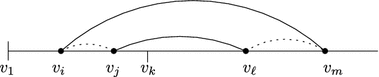
In the next step, we consider a triangle $xyz$ of $\mathcal {T}$. By our assumption on $\mathcal {T}$, we have $\Vert F_{xyz}\Vert =o(1)$. By the choice of $F_{xyo}$, $F_{yzo}$, and $F_{zxo}$, and using Lemma 9, we obtain

$$\begin{aligned} \delta (F_{xyz} + F_{xyo} + F_{yzo}+F_{zxo})=0, \end{aligned}$$

and so we can choose a minimal $(d-3)$-chain $F_{xyzo}$ with

$$\begin{aligned} \delta F_{xyzo} = F_{xyz} + F_{xyo} + F_{yzo}+F_{zxo}. \end{aligned}$$

See Fig. 8 for an illustration. Reasoning as before, we obtain $\max \{ \Vert F_{xyo}\Vert , \Vert F_{yzo}\Vert , \Vert F_{zxo}\Vert \} \ge \tfrac{1}{3} \varphi _{d-2}(\Vert F_{xyzo}\Vert )$, and hence

$$\begin{aligned} \max \{ \Vert F_x\Vert , \Vert F_y\Vert , \Vert F_z\Vert \} \ge \varphi _d\big (\tfrac{1}{2} \varphi _{d-1}\big (\tfrac{1}{3} \varphi _{d-2}\big (\Vert F_{xyzo}\Vert \big )\big )\big ). \end{aligned}$$

We can continue this argument by induction. In the final step, consider a $d$-face $A$ of the triangulation. Corresponding to it, there is a $0$-cochain $F^d_A$. Moreover, for every $(d-1)$-face $B$ of $A$, we have already constructed a $0$-cochain $F_{Bo}$ such that

$$\begin{aligned} \mathop {\max }\limits _{x\in B} \Vert F_x\Vert \ge \varphi _{d}\big (\tfrac{1}{2} \varphi _{d-1}\big (\tfrac{1}{3} \varphi _{d-2}\big (\ldots \tfrac{1}{d} \varphi _1(\Vert F_{Bo}\Vert )\ldots \big )\big )\big ) \end{aligned}$$

and $\delta (F_a + \sum \nolimits _B F_{Bo})=0$. Thus, $F_a + \sum \nolimits _B F_{Bo}$ is a $0$-cocycle, and so it must be either $0$ or all of $V$, the whole vertex set of $\Delta ^{n-1}$. In the former case, we can complete the coning for $A$ by setting $F_{Ao}=0$. If we could do this for all $d$-faces $A$ of $\mathcal {T}$, we would be able to complete the coning, thus reaching a contradiction.

Fig. 8

An illustration of the coning for the boundary of a triangle $xyz$ of $\mathcal {T}$. We use a simplified labeling of the resulting simplices in $\mathcal {Z}^d$. For example, the $0$-chain $F_{xzo}$ by itself does not determine a triangle of $\mathcal {Z}^d$, but only does so together with the $2$-cocycles $o, F_x, F_z$ and the $1$-chains $F_{xz}, F_{xo}, F_{zo}$ that are already determined. We also stress that the coning involves making choices, e.g. between $1$-cochains $F_{yo}$ and $F_{yo}'$ that determine different edges connecting $F_y$ and $o$, and once we have made a choice, we must stick to it when choosing higher-dimensional faces.

Therefore, there must be a $d$-face $A$ such that $F_A + \sum \nolimits _B F_{Bo}=V$. Since $\Vert F_A\Vert =o(1)$, it follows that for some $B\subset A$, we must have $\Vert F_{Bo}\Vert \ge \tfrac{1}{d+1}$. Maximizing over all vertices of $\mathcal {T}$, we conclude

$$\begin{aligned} \mathop {\max }\limits _{x} \Vert F_x\Vert \ge \varphi _{d}\big (\tfrac{1}{2} \varphi _{d-1}\big (\tfrac{1}{3} \varphi _{d-2}\big (\ldots \tfrac{1}{d} \varphi _1\big (\tfrac{1}{d+1}\big )\ldots \big )\big )\big ). \end{aligned}$$

This completes (our outline of) the proof of Proposition 4 in the affine case.

3.5 Gromov’s Method in the Topological Setting

As mentioned in the introduction, the setting of an $n$-point set $P \subseteq {\mathbb {R}}^d$ considered in the previous subsections corresponds to an affine map from the $(n-1)$-simplex $\Delta ^n$ into ${\mathbb {R}}^d$.

Gromov’s method applies to much more general situations. More precisely, it allows for the setting to be generalized in several ways, as we now sketch.

• 1. The simplex $\Delta ^{n-1}$ can be replaced by an arbitrary (finite) simplicial complex $X$. What is needed are lower bounds on the cofilling profile of $X$, which is defined as follows: For $k\ge 0$, let $X_k$ be the set of $k$-dimensional faces of $X$. For each $k$, we have the coboundary operator of $X$ which maps a subset $E\subseteq X_k$ to

  $$\begin{aligned} \delta E:=\big \{f\in X_{k+1}: f \text { contains an odd number of } e\in E\big \}. \end{aligned}$$

  We can identify $E \subseteq X_k$ with a $0/1$-vector indexed by $X_k$, i.e., with an element of the vector space ${\mathbb {Z}}_2^{X_k}$ over the $2$-element field ${\mathbb {Z}}_2$. In more usual (co)homological terminology, this latter vector space is denoted by $C^{k}(X;{\mathbb {Z}}_2)$ and called the space of $k$ -dimensional cochains (with ${\mathbb {Z}}_2$-coefficients), and $\delta$ is a linear map $C^k(X;{\mathbb {Z}}_2)\rightarrow C^{k+1}(X;{\mathbb {Z}}_2)$.

  For a $k$-dimensional cochain $E$, we define $\Vert E\Vert :=|E|/|X_k|$ as the density of $E$ as before, and

  $$\begin{aligned} \varphi ^X_d(\alpha ):=\min \big \{\Vert \delta E\Vert : E\in {\textstyle C^{*}(X;{\mathbb {Z}}_2)} \text{ minimal }, \Vert E\Vert \ge \alpha \big \}, \end{aligned}$$

  where $E$ is minimal if $\Vert E\Vert \le \Vert E+ \delta D\Vert$ for all $D\in C^*(X;{\mathbb {Z}}_2)$.

  The space $\mathcal {Z}^d(X)$ of $d$-dimensional cocycles of $X$ is defined completely analogously to the case of the simplex.

• 2. The target space ${\mathbb {R}}^d$ can be replaced by an arbitrary triangulated $d$-dimensional manifold $Y$, or, even more generally, a ${\mathbb {Z}}_2$-homology manifold. What we need is to be able to compute intersection numbers (modulo 2) between $k$-dimensional chains and $(d-k)$-dimensional chains. Equivalently, we need that Poincaré duality (with ${\mathbb {Z}}_2$ coefficients) holds in $Y$.

• 3. Instead of affine maps, we can allow for arbitrary continuous maps $T:X\rightarrow Y$. Without loss of generality, one can think of $T$ as a piecewise linear map in general position. This is not necessary for the argument, but may help the reader’s intuition. For instance, for such a map, the $T$-image of any $(d-k)$-simplex $\sigma$ of $X$ intersects any $k$-simplex $A$ of $Y$ in a finite number of points in the relative interior of $A$, and the (algebraic, ${\mathbb {Z}}_2$) intersection number of $T(\sigma )$ and $A$ is defined as the number of intersection points modulo $2$.

• 4. Finally, instead of cohomology with ${\mathbb {Z}}_2$-coefficients, one can work with other coefficient rings in the argument. Potentially, this might lead to stronger bounds. We will not discuss this generalization, since on the one hand, it is straightforward, and on the other hand, we would have to talk about orientations everywhere.

The basic structure of the proof remains the same, but we have to change the definition of the cochains $F_A$ appropriately, as follows: If $A$ is a $k$-dimensional simplex in general position, one defines $F_A$ as the set of $(d-k)$-simplices of $X$ whose images under $T$ have odd intersection number with $A$.

Another way of interpreting this construction is as follows: Every $k$-simplex $A$ defines, via Poincaré duality, a $(d-k)$-cochain in $Y$, and this $(d-k)$-cochain pulls back under $T$ to a cochain $F_A$ in $X$.

The basic identity

$$\begin{aligned} \delta F_A=F_{\partial A}=F_{A_0} + F_{A_1} + \cdots + F_{A_k} \end{aligned}$$

(5)

still holds. (This just says that on the level of chains and cochains, Poincaré duality exchanges boundary and coboundary operators).

In other words, every $k$-simplex $A$ in general position defines a $k$-simplex $\Delta _T(A)$ in $\mathcal {Z}^d(X)$ via the intersection number construction. If $Y$ is compact, i.e., has a finite triangulation, then the subspace $\mathcal {W}=\mathcal {W}(T) \subseteq \mathcal {Z}^d(X)$ is defined as the formal ${\mathbb {Z}}_2$-linear combination of the $d$-simplices $\Delta _T(A)$, where $A$ ranges over all $d$-simplices in the triangulation of $Y$. In other words, a $d$-simplex of $\mathcal {Z}^d(X)$ belongs to $\mathcal {W}$ if it equals $\Delta _T(A)$ for an odd number of $d$-simplices $A$ of the triangulation of $Y$.

An equivalent way of defining $\mathcal {W}$ is as follows: The basic identity (5) implies that the map $A\mapsto \Delta _T(A)$ commutes with the boundary operator, i.e., it is a chain map (with ${\mathbb {Z}}_2$-coefficients) from $Y$ to $\mathcal {Z}^d(X)$. Thus, this map also induces a map in homology.

Let $[Y]$ denote the fundamental $d$-dimensional homology class (over ${\mathbb {Z}}_2$) of $Y$. If we fix a triangulation of $Y$, we can take a representative $d$-cycle for $[Y]$ that is the formal ${\mathbb {Z}}_2$-linear combination of all the $d$-simplices of the triangulation. (If $Y$ is not compact, as in the case $Y={\mathbb {R}}^d$, then we have to work with homology with infinite supports.) Then $\mathcal {W}=\mathcal {W}(f)$ is defined as the image under the map $\Delta _T$ of $[Y]$, i.e., formally, it is a $d$-dimensional cycle (with ${\mathbb {Z}}_2$-coefficients) in $\mathcal {Z}^d(X)$.

As before, the Almgren–Dold–Thom Theorem implies that this cycle is homologically nontrivial, so it cannot be contracted.

On the other hand, if every point of $Y$ were covered by the $T$-images of “too few” $d$-simplices of $X$, then the same combinatorial coning as before would yield a contradiction (with the precise meaning of “too few” depending on the cofilling profile of $X$). Again, the combinatorial coning can also be viewed as an actual topological contraction of $\mathcal {W}$, considered as a subspace of $\mathcal {Z}^d(X)$, to the point $o$.

If $Y$ is unbounded, or if we are guaranteed that there is a point of $Y$ that is not covered by the image of $T$, then the same argument as before shows that

$$\begin{aligned} \mathop {\max }\limits _{y} \Vert F_y\Vert \ge \varphi ^X_{d}\big (\tfrac{1}{2} \varphi ^X_{d-1}\big (\tfrac{1}{3} \varphi ^X_{d-2}\big (\ldots \tfrac{1}{d} \varphi ^X_1\big (\tfrac{1}{d+1}\big )\ldots \big )\big )\big ), \end{aligned}$$

where the maximum is over all vertices $y$ of the triangulation of $Y$. (If $Y$ is not unbounded and if every point in $Y$ is covered by the $T$-images of some $d$-simplices of $X$, then we have to choose the apex $o$ of the coning differently (not as the empty cocycle), which yields a weaker bound.)

In particular, if $X$ is a ${\mathbb {Z}}_2$ -cohomological expander, i.e., if $\varphi _i^X(\alpha )/\alpha$ is bounded away from zero for all $i$, then there is some point of $Y$ that is covered by a positive fraction of all $d$-simplices of $X$ (with a constant depending on the cofilling profile of $X$).

We remark that for the coning argument, we again choose the triangulation $\mathcal {T}$ to be sufficiently fine with respect to the map $T$, i.e., we assume that for every simplex $A$ of the triangulation of dimension $\dim A >0$, we have $\Vert F_A\Vert =o(1)$. If the map $T$ is very complicated (i.e., if we need a very fine subdivision of $X$ to approximate $T$ by a PL map), then the triangulation $\mathcal {T}$ may require a huge number of simplices, so it is important that the whole argument is completely independent of the number of simplices in the triangulation $\mathcal {T}$.

4 The cofilling profile in the d = 2 case

Here we prove Theorem 5, which asserts that

$$\begin{aligned} \varphi _2(\alpha ) \ge f(\alpha ):=\tfrac{3}{4}\big (1-\sqrt{1-4\alpha }\big )(1-4\alpha ). \end{aligned}$$

Since $d=2$, we deal with the size of the coboundary for an edge set $E$ of a graph. The minimality of $E$ means that no edge cut has density more than $\frac{1}{2}$ in this graph; in other words, for every $S\subseteq V$, the number of edges of $E$ going between $S$ and $V\setminus S$ is at most $\frac{1}{2}|S|\cdot |V\setminus S|$.

As we have remarked at the end of Sect. 2, the minimality of $E$ is a complicated property, computationally hard to test, for example. So we will only use it for singleton sets $S$. Thus, we will actually show that $\Vert \delta E\Vert \ge f(\alpha )$ (ignoring terms tending to $0$ as $n\rightarrow \infty$) for every $E$ with $\Vert E\Vert \ge \alpha$ and $\deg _E(v)\le \frac{n}{2}$ for all $v\in V$ (where $\deg _E(v)$ denotes the number of neighbors of $v$ in the graph $(V,E)$).

Before proceeding with the proof of Theorem 5, let us remark that this relaxation (i.e., ignoring all non-singleton $S$) already prevents us from obtaining a tight bound for $\varphi _2$. For example, let us partition $V$ into sets $V_1,V_2,V_3$, where $|V_1|=\alpha n$ and $|V_2|=\frac{n}{2}$, and let $E$ consist of all edges connecting $V_1$ to $V_2$. This $E$ is not minimal, but it does satisfy the degree condition. One easily checks that $\Vert E\Vert =\alpha$ and $\Vert \delta E\Vert =3 \alpha (\frac{1}{2}-\alpha )=\frac{3}{2}\alpha -3\alpha ^2$, which is smaller than the suspected tight bound for $\varphi _2$ from Proposition 7. However, at least the leading term is correct.

Now we proceed with the proof. Given $E$, let $m_i$ denote the number of triples $f\in {V\atopwithdelims ()3}$ that contain $i$ edges of $E$, $i=1,2,3$; we have $|\delta E|= m_1+m_3$ by definition. An easy inclusion–exclusion consideration shows that

$$\begin{aligned} |\delta E| = (n-2)|E|-\textstyle \sum \limits _{v\in V}\deg _E(v)(\deg _E(v)-1)+ 4t, \end{aligned}$$

(6)

where $t$ denotes the number of triangles in the graph $(V,E)$. Indeed, to check (6), it suffices to discuss how many times a triple $f\in {V\atopwithdelims ()3}$ containing exactly $i$ edges $e\in E$ contributes to the right-hand side, $i=1,2,3$. For $i=1$, such an $f$ is only counted once in the term $(n-2)|E|$, which counts the number of ordered pairs $(e,v)$, where $e\in E$ and $v\in V\setminus e$. A triple $f$ with $i=2$ is counted twice in the term $(n-2)|E|$, but it is also counted twice in $\sum \nolimits _{v\in V}\deg _E(v)(\deg _E(v)-1)$, and thus its total contribution is zero. Finally, for $i=3$, where $f$ induces a triangle, it is counted three times in $(n-2)|E|$, six times in $\sum \nolimits _{v\in V}\deg _E(v)(\deg _E(v)-1)$, and four times in $4t$, so altogether it contributes $+1$ as it should.

As the next simplification, we will ignore the triangles, as well as the difference between $\deg _E(v)(\deg _E(v)-1)$ and $\deg _E(v)^2$, and we will use (6) in the form

$$\begin{aligned} |\delta E| \ge (n-2)|E|-\textstyle \sum \limits _{v\in V}\deg _E(v)^2. \end{aligned}$$

(7)

Since $|E|$ is given, it remains to maximize $\sum \nolimits _{v\in V}\deg _E(v)^2$, which is done in the next lemma.

Lemma 10

Let $\alpha \le \frac{1}{4}$. Let $(V,E)$ be a graph on $n$ vertices with $|E|=\alpha {n\atopwithdelims ()2}$ and $\deg _E(v)\le \frac{n}{2}$ for all $v\in V$. Then

$$\begin{aligned} \textstyle \sum \limits _{v\in V}\deg _E(v)^2 \le \big (\tfrac{\sigma }{4} (1+2\sigma -4\sigma ^2)+o(1)\big )n^3, \end{aligned}$$

where $\sigma =(1-\sqrt{1-4\alpha })/2$ is one of the two roots of $\sigma ^2-\sigma +\alpha =0$.

Proof

Let $(V,E)$ be the given graph with $n$ vertices and $|E|=\alpha \left( {\begin{array}{c}n\\ 2\end{array}}\right)$ edges. By a sequence of transformations that do not change the number of edges and that do not decrease the sum of squared degrees, we convert it to a particular form.

Let us number the vertices $v_1,\ldots ,v_n$ so that $d_1\ge d_2\ge \cdots \ge d_n$, where $d_i:=\deg _E(v_i)$. We note that for $d_i\ge d_j$, we have $(d_i+1)^2+(d_j-1)^2 > d_i^2+d_j^2$, and thus a transformation that changes $d_i$ to $d_i+1$ and $d_j$ to $d_j-1$ and leaves the rest of the degrees unchanged increases the sum of squared degrees.

For an edge $e=\{v_i,v_j\}$ with $i<j$, we call $v_i$ the left end of $e$ and $v_j$ the right end.

• (i) Let $k$ be such that $d_1=d_2=\cdots =d_k=\lfloor \frac{n}{2}\rfloor$, while $d_{k+1}<\lfloor \frac{n}{2}\rfloor$. Then we may assume that the left ends of all edges are among $v_1,\ldots ,v_{k+1}$.

  Indeed, if there is an edge $\{v_i,v_j\}$, $i>k+1$, we can replace it with the edge $\{v_{k+1},v_j\}$. This increases $\sum \nolimits _{i=1}^{k+1} d_i$ (and possibly increases $k$), so after finitely many steps, we achieve the required condition.

• (ii) We may assume that every two vertices among $v_1,\ldots ,v_k$ are connected.

  Proof: We may assume that (i) holds. Since we assume $\alpha \le \frac{1}{4}$, we have $k\le \lfloor \frac{n}{2}\rfloor$. Let us suppose $\{v_i,v_j\}\not \in E$, $1\le i<j\le k$. Since $d_i=d_j=\lfloor \frac{n}{2}\rfloor$, each of $d_i,d_j$ is connected to at least two vertices among $v_{k+1},\ldots ,v_n$. So we may assume $\{v_i,v_{\ell }\}\in E$, $\{v_j,v_m\}\in E$, $\ell ,m\ge k+1$, $\ell \ne m$. We also have $\{v_{\ell },v_m\}\not \in E$ (according to (i)). Thus, we can delete the edges $\{v_i,v_{\ell }\}$ and $\{v_j,v_{m}\}$ and add the edges $\{v_i,v_j\}$ and $\{v_{\ell },v_m\}$.

  

  This increases the number of edges on $\{v_1,\ldots ,v_k\}$, which cannot decrease by the transformations in (i), so after finitely many steps, we achieve both (i) and (ii).

• (iii) We may assume that the right neighbors of each $v_i$, $1\le i\le k$, form a contiguous interval $v_{i+1},v_{i+2},\ldots ,v_{\lfloor n/2\rfloor +1}$.

  Indeed, if $v_i$ is connected to some $v_{\ell +1}$ and not to $v_{\ell }$, $\ell >k$, we can replace the edge $\{v_i,v_{\ell +1}\}$ with $\{v_i,v_{\ell }\}$. This increases the sum of squared vertex degrees, and thus after finitely many steps, we can achieve (i)–(iii).

A graph satisfying (i)–(iii) is almost completely determined by its number of edges, except possibly for the neighbors of the vertex $v_{k+1}$. Each of $v_1,\ldots ,v_k$ is connected to the first $\frac{n}{2}$ vertices, and there are no other edges, except possibly for those incident to $v_{k+1}$. Counting the left ends of edges, we have $\alpha {n\atopwithdelims ()2}=|E|=kn/2-{k\atopwithdelims ()2}+O(n)$.

Writing $k=\sigma n$, we obtain $\sigma =(1-\sqrt{1-4\alpha })/2+o(1)$. The sum of the squared degrees is then $k\frac{n^2}{4}+(\frac{n}{2}-k)k^2+O(n^2)=\big ( \frac{\sigma }{4}(1+2\sigma -4\sigma ^2)+o(1)\big )n^3$. Lemma 10 is proved. $\square$

Proof of Theorem 5

Let $E\subseteq \left( {\begin{array}{c}V\\ 2\end{array}}\right)$ be minimal with $|E|=\alpha \left( {\begin{array}{c}n\\ 2\end{array}}\right)$. By (7) and Lemma 10,

$$\begin{aligned} |\delta E|&\ge (n-2)|E| - \textstyle \sum \limits _{v\in V} \deg _E(v)^2\\&\ge 3\alpha \big (\begin{array}{l}n\\ 3\end{array}\big ) - \big (\frac{\sigma }{4}(1+2\sigma -4\sigma ^2)+o(1)\big ) n^3\\&= \frac{3}{2}\big (2\sigma -2\sigma ^2-\sigma (1+2\sigma -4\sigma ^2) +o(1)\big )\big (\begin{array}{l}n\\ 3\end{array}\big )\\&= \frac{3}{2}\big (\sigma (1-2\sigma )^2+o(1)\big )\big (\begin{array}{l}n\\ 3\end{array}\big ) = \frac{3}{4}\big (\big (1-\sqrt{1-4\alpha }\big )(1-4\alpha )+o(1)\big )\big (\begin{array}{l}n\\ 3\end{array}\big ), \end{aligned}$$

as claimed. $\square$

A Promising Relaxation? As we have seen, in order to establish the tightness of the upper bound from Proposition 7, one has to use the minimality condition in a stronger way than we did in the above proof. On the other hand, it seems possible that the other relaxation we have made in that proof, namely, ignoring triangles, need not cost us anything. In other words, while in $\delta E$ we count triples containing 1 or 3 edges, perhaps the example in Proposition 7 also minimizes, over all minimal $E$ of a given size, the number of triples containing exactly one edge. This might be easier to prove, and triangles would be dealt with implicitly, since the example has no triangles.

On Gromov’s “ $\frac{2}{3}$ -Bound”. Sect. 3.7 of  [9] claims the lower bound $\Vert (\partial ^1)^{-1}_\mathrm{fil}\Vert (\beta )\le \frac{2}{3(1-\sqrt{\beta })}$ (which would yield $\varphi _2(\alpha ) \ge \tfrac{3}{2}\alpha -(\tfrac{3}{2})^{3/2}\alpha ^{3/2}+\tfrac{9}{8}\alpha ^2-O(\alpha ^{5/2})$.

The argument as given does not seem to work, however (although it is also possible that we misunderstood something). It is supposed to be based on an inequality (the fifth displayed formula in Sect. 3.7, derived from the Loomis–Whitney inequality), which seems correct and is re-stated for $i=1$ two lines below. In the language of graphs, the $i=1$ case is equivalent to $\sum \nolimits _{\{u,v\}\in {V\atopwithdelims ()2}} \deg _E(u)\deg _E(v)\le 2\frac{n-1}{n}|E|^2$.

However, the proof of the “$\frac{2}{3}$-bound” seems to employ a similar inequality for $i=2$, which would claim that $\sum \nolimits _{\{u,v\}\in {V\atopwithdelims ()2}}\sqrt{\deg _E(u)\deg _E(v)}\le 2|E|^{3/2}$. This is false, though (a graph as in the upper bound example, i.e., a complete bipartite graph with parts of very unequal size, is a counterexample). Probably this kind of proof can be saved, since it seems sufficient to take the last sum over $\{u,v\}\in E$, instead of all pairs, and then such an inequality is apparently true (but it does not seem to follow from Loomis–Whitney in a direct way).

5 The Cofilling Profile for d > 2

In this section we prove Theorem 6, a lower bound on $\varphi _3$. We begin with an auxiliary fact concerning links of vertices.

Observation 11

If $E\subseteq {V\atopwithdelims ()d}$ is a minimal system, then $\mathop {\mathrm{lk}}\nolimits (v,E)$ is also minimal, for every vertex $v\in V$.

Proof

For a set system $F$ on $V$, let us write $F_{\setminus v}:= \{s\in F:v\not \in F\}$.

We want to verify that for each $C\subseteq {V\atopwithdelims ()d-2}$, $\mathop {\mathrm{lk}}\nolimits (v,E)$ contains at most half of $\delta C$. The sets of $\mathop {\mathrm{lk}}\nolimits (v,E)$ do not contain $v$, and so only sets of $(\delta C)_{\setminus v}$ may belong to $\mathop {\mathrm{lk}}\nolimits (v,E)$. But we have $(\delta C)_{\setminus v} = (\delta C_{\setminus v})_{\setminus v}$, and so we may restrict our attention to systems $C$ whose sets all avoid $v$.

Let $D:=C*v:=\{c\cup \{v\}:c\in C\}$. We have $\delta D= ((\delta C)_{\setminus v})*v$. Now $E$ contains at most half of the sets of $\delta D$ by minimality, so $\mathop {\mathrm{lk}}\nolimits (v,E)$ contains at most half of the sets of $(\delta C)_{\setminus v}$ as claimed. $\square$

In the proof of Theorem 6, we consider a minimal system $E\subseteq {V\atopwithdelims ()3}$, $\Vert E\Vert =\alpha$, and we want to show that it has a large coboundary. Conceptually, the proof splits into two cases: The first one deals with the situation where most of the triples $e\in E$ are incident to vertices of very large degrees. The second one concerns the situation where the maximum vertex degree is not much larger than the average vertex degree.

Dealing with High-Degree Vertices. We begin with the first case, with a significant share of high-degree vertices. Here we rely on the basic cofilling bound, which we are going to apply to the links of high-degree vertices (the links are minimal by Observation 11). From the sets in the coboundaries of the links we are going to obtain sets of $\delta E$; some care is needed to avoid counting a single $f\in \delta E$ several times.

It is interesting to note that in this way we get a lower bound for $\varphi _3$ that has a correct limit behavior as $\alpha \rightarrow 0$, although for the links we employ the basic cofilling bound, which is far from correct for small $\alpha$’s. This can be explained as follows: for those systems $E$ that are near-extremal for $\varphi _3$, the relevant vertex links are so large that the basic cofilling bound is almost tight for them.

We present the first part of the proof for $d$-tuples instead of triples, since specializing to triples would not make the argument any simpler.

Lemma 12

Let $E$ be a minimal system of $d$-tuples on $V=\{v_1,v_2,\ldots ,v_n\}$, let $\alpha :=\Vert E\Vert$, let $r=\beta n$ be a parameter, and let $E_\mathrm{hi}\subseteq E$ consist of those $e\in E$ that contain at least one vertex among $v_1,\ldots ,v_r$. Let $F_\mathrm{hi}$ be the set of those $f\in \delta E$ that contain at least one vertex among $v_1,\ldots ,v_r$. Then

$$\begin{aligned} \Vert F_\mathrm{hi}\Vert \ge \frac{d+1}{d} \alpha _\mathrm{hi} - \frac{(d+1)d}{2} \beta ^2-(d+1)\alpha \beta - O(n^{-1}), \end{aligned}$$

where $\alpha _\mathrm{hi}:=\Vert E_\mathrm{hi}\Vert$.

Proof

Let $v\in V$ be a vertex, and let us write $L_v:=\mathop {\mathrm{lk}}\nolimits (v,E)$. Then, by Observation 11, $L_v$ is minimal, and thus $\Vert \delta L_v\Vert \ge \Vert L_v\Vert$ by the basic bound on $\varphi _{d-1}$. In terms of cardinalities, we can write this inequality as $|\delta L_v|\ge \frac{n-d+1}{d}|L_v|$.

Let us consider some $e\in \delta L_v$. We observe that if $v\not \in e$ and $e\not \in E$, then $e\cup \{v\}\in \delta E$. There are exactly $|L_v|$ sets $e\in \delta L_v$ that contain $v$, and so the number of $f\in \delta E$ that contain $v$ is at least

$$\begin{aligned} \frac{n-d+1}{d} |L_v|-|L_v|-|E|. \end{aligned}$$

(8)

To prove the lemma, we would like to sum this bound over $v=v_1,v_2,\ldots ,v_r$, but in this way, one $f\in \delta E$ might be counted several times. In order to avoid this, for each $v_i$ we will count only those $f\in \delta E$ that contain $v_i$ and avoid $v_1,\ldots ,v_{i-1}$.

In this way, from the term (8) for $v=v_i$ we need to subtract the number of $f\in \delta E$ that contain both $v_i$ and some $v_j$, $j<i$. A trivial upper bound on this number is $(i-1){n-2\atopwithdelims ()d-1}$. Hence

$$\begin{aligned} |F_\mathrm{hi}|&\ge \textstyle \sum \limits _{i=1}^r(\big (\tfrac{n-d+1}{d}-1\big )|L_{v_i}|- (i-1) \big (\begin{array}{l}n-2\\ d-1\end{array}\big ) -|E|)\\&\ge \frac{n}{d} \big (\textstyle \sum \limits _{i=1}^r |L_{v_i}|\big )- \frac{\beta ^2}{2} n^2 \big (\begin{array}{c}n\\ d-1\end{array}\big ) - \beta n|E|- O(n^d). \end{aligned}$$

(For the second inequality, $-2\sum \nolimits _{i=1}^r|L_{v_i}|$ is subsumed in the $O(n^d)$-term.) Now $\sum \nolimits _{i=1}^r |L_{v_i}|\ge |E_\mathrm{hi}|$. We finally divide by $n\atopwithdelims ()d+1$ in order to pass to the density (normalized size) measure $\Vert .\Vert$, and we obtain the lemma. $\square$

Dealing with Low-Degree Vertices. Next, we will show that if the vertex degrees of $E$ do not exceed the average vertex degree by too much, then $\delta E$ is even significantly larger than in the upper bound example from Proposition 7. Here it is important for the argument that we deal with triples.

In this case, we are going to count the sets of the coboundary using two-term inclusion-exclusion, similar to the case $d=2$ in the preceding section. This leads to bounding from above the sum of squares of the degrees of pairs of vertices. For this, by a suitable double counting, we use the assumption of low vertex degrees, and also the fact that the degrees of all pairs are bounded by $\frac{n}{2}$, which follows from the minimality of $E$.

Lemma 13

Let $d=3$ and let $E\subseteq {V\atopwithdelims ()3}$. Suppose that $\deg _E(p)\le \frac{n}{2}$ for each pair $p=\{u,v\}$ of vertices, and that $\deg _E(v)\le \sigma {n\atopwithdelims ()2}$ for each vertex $v$. Then

$$\begin{aligned} \Vert \delta E\Vert \ge (2-O(\sigma ^{1/3}))\Vert E\Vert . \end{aligned}$$

Proof

Similar to the graph case, we will count only those $4$-tuples in $\delta E$ that contain exactly one $e\in E$. For each $e\in E$, we count $n-3$ potential $4$-tuples, and we subtract $1$ for each $e'\in E$ sharing a pair with $e$. Thus,

$$\begin{aligned} |\delta E|\ge (n-3)|E|-\textstyle \sum \limits _{p\in {V\atopwithdelims ()2}} \deg _E(p)^2. \end{aligned}$$

We need to estimate the second term.

We choose a threshold parameter $\tau$, which we think of as being much larger than $\sigma$ but still small, and we call a pair $p$ heavy if $\deg _E(p)\ge \tau n$, and light otherwise.

Each $e\in E$ shares a light pair with at most $3\tau n$ other $e'\in E$, and so the contribution of light pairs is bounded as follows:

$$\begin{aligned} \textstyle \sum \limits _{p \mathrm {~light}} \deg _E(p)^2 \le 3\tau n |E|. \end{aligned}$$

Let $E_k$ be the number of $e\in E$ with exactly $k$ heavy pairs, $k=0,1,2,3$. Since each heavy pair has degree at most $\frac{n}{2}$, reasoning as above, we can bound the contribution of the heavy pairs as

$$\begin{aligned} \textstyle \sum \limits _{p \mathrm {~heavy}} \deg _E(p)^2 \le \frac{n}{2} (|E_1|+2|E_2|+3|E_3|). \end{aligned}$$

We aim at showing that $E_2\cup E_3$ is small.

Let us consider a vertex $v\in V$ and see how many $e\in E_2\cup E_3$ can be incident to it. More precisely, we want to estimate $m_v$, the number of $e\in E_2\cup E_3$ that have two heavy pairs incident to $v$.

Let $\deg _E(v)=\sigma _v {n\atopwithdelims ()2}$, where $\sigma _v\le \sigma$, and let us consider the graph $G_v:=(V,\mathop {\mathrm{lk}}\nolimits (v,E))$. The heavy pairs incident to $v$ correspond to the heavy vertices of $G_v$, i.e., vertices of degree at least $\tau n$, and $m_v$ is the number of pairs in $G_v$ connecting two heavy vertices. By simple counting, $G_v$ has at most $\frac{\sigma _v n}{\tau }$ heavy vertices, and thus $m_v\le (\frac{\sigma _v n}{\tau })^2/2 \le \frac{\sigma }{\tau ^2} |\mathop {\mathrm{lk}}\nolimits (v,E)|$.

Summing over all vertices $v$, we have $|E_2|+|E_3|\le \frac{3\sigma }{\tau ^2} |E|$. Altogether we thus have

$$\begin{aligned} \textstyle \sum \limits _{p\in {V\atopwithdelims ()2}} \deg _E(p)^2\le 3\tau n |E| + \frac{n}{2} |E|+ O\big (\tfrac{\sigma }{\tau ^2}\big )n|E|. \end{aligned}$$

Finally, setting $\tau := \sigma ^{1/3}$ and normalizing by ${n\atopwithdelims ()3}$, we obtain the claim of the lemma. $\square$

Proof of Theorem 6

This is a straightforward consequence of Lemmas 12 and 13. We consider a minimal $E\subseteq {V\atopwithdelims ()3}$ with $\Vert E\Vert =\alpha$. We enumerate the vertices of $V$ as $v_1,\ldots ,v_n$ in the order of decreasing degrees. For a suitable parameter $\beta >\alpha$ (depending on $\alpha$), we set $r:=\beta n$, we let $E_\mathrm{hi}$ be those $e\in E$ that contain a vertex among $v_1,\ldots ,v_r$, and let $E_\mathrm{lo}:=E\setminus E_\mathrm{hi}$.

We have $\sum \nolimits _{i=1}^n\deg _E(v_i) = 3|E|$, and so the degrees of the vertices $v_r,v_{r+1},\ldots ,v_n$ are bounded from above by $\frac{3|E|}{r}$. Hence Lemma 13 with $\sigma := \alpha /\beta$ gives $\Vert \delta E_\mathrm{lo}\Vert \ge (2-(\alpha /\beta )^{1/3}) \alpha _\mathrm{lo}$, where $\alpha _\mathrm{lo}:=\Vert E_\mathrm{lo}\Vert$.

Let $F_\mathrm{hi}$ be the set of those $f\in \delta E$ that contain a vertex among $v_1,\ldots ,v_r$; then Lemma 12 yields $\Vert F_\mathrm{hi}\Vert \ge \frac{4}{3}\alpha _\mathrm{hi} - O(\beta ^2)$ (the $\alpha \beta$ term in the lemma is insignificant since we assume $\alpha \le \beta$).

We now observe that if some $f\in \delta E_\mathrm{lo}$ does not contain any of $v_1,\ldots ,v_r$, then it belongs to $\delta E$ (since it cannot contain any $e\in E_\mathrm{hi}$). The number of $f\in \delta E_\mathrm{lo}$ that do contain some vertex among $v_1,\ldots ,v_r$ is bounded by $r |E_\mathrm{lo}|$. Altogether we thus have

$$\begin{aligned} \Vert \delta E\Vert&\ge \Vert F_\mathrm{hi}\Vert +\Vert \delta E_\mathrm{lo}\Vert -O(\beta \alpha _\mathrm{lo})\\&\ge \tfrac{4}{3}\alpha _\mathrm{hi} - O(\beta ^2) +\big (2-(\alpha /\beta )^{1/3}\big ) \alpha _\mathrm{lo}\\&\ge \tfrac{4}{3}\alpha -O(\beta ^2) + \big (\tfrac{2}{3} - O((\alpha /\beta )^{1/3})\big )\alpha _\mathrm{lo}. \end{aligned}$$

If we set $\beta := C\alpha$ for a sufficiently large constant $C$, then the term $O((\alpha /\beta )^{1/3})$ becomes smaller than $\frac{2}{3}$, and the whole term involving $\alpha _\mathrm{lo}$ is nonnegative. Thus, we are left with $\Vert \delta E\Vert \ge \frac{4}{3}\alpha -O(\alpha ^2)$ as claimed.$\square$

6 Pagodas and a Better Bound on $\varvec{c_3}$

We recall the lower bound for the Bárány constant $c_d$ from Proposition 4:

$$\begin{aligned} c_d\ge \varphi _{d}\big (\tfrac{1}{2} \varphi _{d-1}\big (\tfrac{1}{3} \varphi _{d-2}\big (\ldots \tfrac{1}{d} \varphi _1(\tfrac{1}{d+1})\ldots \big )\big )\big ), \end{aligned}$$

(9)

As a case study, we will concentrate on $c_3$, the first open case. The various numerical bounds are as follows.

• Gromov’s bound, obtained from (9) via the basic cofilling bound and the precise value of $\varphi _1$, is

  $$\begin{aligned} c_3\ge \frac{1}{16}= 0.0625. \end{aligned}$$

• For comparison, the best lower achieved by other methods, due to Basit et al. [5], is

  $$\begin{aligned} c_3\ge 0.05448. \end{aligned}$$

• With maximal optimism, assuming that the upper bounds of Proposition 7 are tight for $\varphi _2$ and $\varphi _3$, (9) would give

  $$\begin{aligned} c_3{\,\mathop {\ge }\limits ^{??}\,}0.0877695. \end{aligned}$$

• However, the best upper bound, which we suspect to be the truth, only gives

  $$\begin{aligned} c_3\le 4!/4^4=\tfrac{3}{32}= 0.09375. \end{aligned}$$

Here we will show how the lower bound for $c_3$ can be improved beyond (9). The specific number we achieve is not very impressive: $c_3\ge 0.06332$. However, it is important that the proof relies only on the basic cofilling bounds on $\varphi _2$ and $\varphi _3$. If better lower bounds on $\varphi _2$ or $\varphi _3$ could be proved in suitable ranges of $\alpha$, which would improve the lower bound (9), we would automatically get a further (slight) improvement from the proof below; in this sense, the method is “orthogonal” to bounds on the cofilling profiles.

We begin by returning to the argument in Sect. 3.4 that proves (9), and for simplicity, we specialize to the $d=3$ case. In that argument, we considered a tetrahedron $wxyz$ in the triangulation $\mathcal {T}$, with the corresponding set systems (cochains) $F_A\subseteq {V\atopwithdelims ()5-|A|}$ for all nonempty sets $A\subseteq S:=\{w,x,y,z\}$. We have $\Vert F_A\Vert =o(1)$ unless $|A|=1$. We also produced the set systems $F_{Ao}\subseteq {V\atopwithdelims ()4-|A|}$ satisfying the relations

$$\begin{aligned} \delta F_{Ao}=F_A+\textstyle \sum \limits _B F_{Bo}, \end{aligned}$$

(10)

where the sum is over all $B\subset A$ of size $|A|-1$. Moreover, the crux of the argument was the existence of a tetrahedron $wxyz$ for which we also have

$$\begin{aligned} F_S+\textstyle \sum \limits _{B\in {S\atopwithdelims ()3}} F_{Bo}=V. \end{aligned}$$

(11)

We introduce the notation $X\approx Y$ for sets $X,Y$ of $k$-tuples, meaning that $|X+Y|=o(n^{k})$, or in other words, $\Vert X+Y\Vert =o(1)$. We eliminate the sets $F_A$ with $|A|\ne 1$ from our considerations, since they are all small; then (10) and (11) become $\approx$ relations among the various $F_{Ao}$.

We introduce a definition reflecting these relations; we chose to call the resulting object, a structure made of cochains of various dimensions, a pagoda. In order to make the notation more intuitive, we distinguish sets of various cardinalities by different letters (with indices), writing $V$ for sets of vertices (0-cochains), $E$ for sets of edges (1-cochains), $F$ for sets of triples (2-cochains), and $G$ for sets of four-tuples. We also change the indexing of the sets into an (isomorphic but) more convenient one. This leads to the following definition.

Definition 14

A ($3$-dimensional) pagoda over $V$ consists of vertex sets $V_1,V_2,V_3,V_4\subseteq V$, edge sets $E_{12},E_{13},\ldots ,E_{34}\subseteq {V\atopwithdelims ()2}$, sets $F_{123}$, $F_{124}$, $F_{134}$, $F_{234} \subseteq {V\atopwithdelims ()3}$ of triples, and a set $G=G_{1234}\subseteq {V\atopwithdelims ()4}$ of $4$-tuples (the top of the pagoda). The sets $V_i$, $E_{ij}$ and $F_{ijk}$ are minimal and they satisfy the following relations (here $i,j,k$ denote mutually distinct indices):

$$\begin{aligned} V_1+V_2+V_3+V_4\approx V,\ \delta V_i\approx \textstyle \sum \limits _j E_{ij},\ \delta E_{ij} \approx \textstyle \sum \limits _k F_{ijk},\ \delta F_{ijk}\approx G. \end{aligned}$$

Thus, the argument of Proposition 4 shows that $c_3\ge c^{\mathrm{top}}_3\ge \lim \inf _{|V|\rightarrow \infty }\min \Vert G\Vert$, where the minimum is over tops $G$ of pagodas over $V$.

We know of no example of a pagoda whose top is smaller than the best known upper bound for $c_3$, i.e., $\Vert G\Vert =\tfrac{3}{32}$. So it is possible that the value of $c_3$ can be determined precisely using a combinatorial analysis of pagodas. Unfortunately, we have only a much weaker result.

Proposition 15

The top $G$ of every pagoda satisfies, for all $n$ sufficiently large, $\Vert G\Vert \ge \frac{1}{16}+\varepsilon _0$, for a positive constant $\varepsilon _0> 0.00082$. Consequently, $c_3\ge c^{\mathrm{top}}_3\ge \frac{1}{16}+\varepsilon _0> 0.06332$.

A similar, but more complicated, argument probably also works for higher-dimensional pagodas.

Remark

Developing the ideas from the forthcoming proof of Proposition 15, one can set up a rather complicated optimization problem, whose optimum provides a lower bound for $c^{\mathrm{top}}_3$. However, solving this (non-convex) optimization problem rigorously seems rather difficult. Numerical computations indicate that the optimum is approximately $0.0703125$. This would be an improvement much more significant than the one in Proposition 15, but still far from the suspected true value of $c_3$.

Proof of Proposition 15

We begin by an outline of the argument. We consider a pagoda with $\Vert G\Vert \le \frac{1}{16}+\varepsilon _0$, where $\varepsilon _0\ge 0$ is a yet unspecified (small) parameter. Reasoning essentially as in the derivation of (9) and using the basic bound for $\varphi _3$ and $\varphi _2$ and the true value of $\varphi _1$, we find that no $\Vert E_{ij}\Vert$ and no $\Vert \delta E_{ij}\Vert$ may be significantly larger than $\frac{1}{8}$, and no $V_i$ may occupy much more than $\frac{1}{4}$ of the vertex set. Hence the $V_i$ are almost disjoint and have sizes close to $\frac{1}{4}$. Then one can argue that almost all edges of $E_{12}$, say, have to go between $V_1$ and $V_2$, as in the following picture:

Then, however, the coboundary $\delta E_{12}$ contains almost all triples of the form indicated in the picture, and thus $\Vert \delta E_{12}\Vert$ is close to $\frac{3}{16}$, rather than to $\frac{1}{8}$, which is a contradiction showing that $\varepsilon _0$ cannot be taken arbitrarily small.

Now we proceed with a more detailed and more quantitative argument. Since $\Vert G\Vert \le \frac{1}{16}+\varepsilon _0$ and $G\approx \delta F_{ijk}$, we have $\Vert F_{ijk}\Vert \le \frac{1}{16}+\varepsilon _0$ according to the basic bound for $\varphi _3$ (ignoring, for simplicity, the $o(1)$ terms coming from $\approx$). Further, since each $\delta E_{ij}$ is a sum of two $F_{ijk}$’s, the basic bound for $\varphi _2$ gives

$$\begin{aligned} \Vert E_{ij}\Vert \le \tfrac{1}{8}+2\varepsilon _0,\ \ \ 1\le i<j\le 4. \end{aligned}$$

Similarly, since each $\delta V_i$ is the sum of three $E_{ij}$’s, and since $\varphi _1(\alpha )=2\alpha (1-\alpha )$, we get

$$\begin{aligned} \Vert V_i\Vert \le \tfrac{1}{4}+\varepsilon _1, \end{aligned}$$

(12)

where $\varepsilon _1=\frac{1}{4}\big (1-\sqrt{1-48\varepsilon _0}\big )= 6\varepsilon _0+72\varepsilon _0^2+O(\varepsilon _0^3)$ is given by the equation $\varphi _1(\frac{1}{4}+\varepsilon _1)=3(\frac{1}{8}+2\varepsilon _0)$.

Next, let $E^\mathrm{dbl}_{ij}$ be the set of edges $e\in E_{ij}$ that belong to both $\delta V_i$ and $\delta V_j$, and let $E^\mathrm{sgl}_{ij}$ consist of those $e\in E_{ij}$ that belong to exactly one of $\delta V_i,\delta V_j$.

Using $\delta V_i\approx \sum \nolimits _{j} E_{ij}$ and summing over $i=1,\ldots ,4$, we have

$$\begin{aligned} \textstyle \sum \limits _{i=1}^4\Vert \delta V_i\Vert \le 2\textstyle \sum \limits _{i<j}\Vert E^\mathrm{dbl}_{ij}\Vert + \textstyle \sum \limits _{i<j}\Vert E^\mathrm{sgl}_{ij}\Vert . \end{aligned}$$

(13)

For every $i$, we have, using (12),

$$\begin{aligned} \Vert V_i\Vert \ge 1-\textstyle \sum \limits _{j\ne i}\Vert V_j\Vert \ge 1-3(\tfrac{1}{4}+\varepsilon _1)\ge \tfrac{1}{4}-3\varepsilon _1. \end{aligned}$$

Hence the left-hand side of (13) is at least $4\varphi _1\big (\frac{1}{4}-3\varepsilon _1\big )=4(\frac{3}{8}-\varepsilon _2)$, where $\varepsilon _2$ is defined by the last equality (we get $\varepsilon _2=18\varepsilon _0+864\varepsilon _0^2+O(\varepsilon _0^3)$).

Further, for every $i<j$ we have $\Vert E^\mathrm{dbl}_{ij}\Vert +\Vert E^\mathrm{sgl}_{ij}\Vert \le \Vert E_{ij}\Vert \le \frac{1}{8}+2\varepsilon _0$. Summing this inequality over the six pairs $i,j$ and subtracting the result from (13), we arrive at

$$\begin{aligned} 4\left( \tfrac{3}{8}-\varepsilon _2\right) -\tfrac{6}{8}-6\cdot 2\varepsilon _0\le \textstyle \sum \limits _{i<j}\Vert E^\mathrm{dbl}_{ij}\Vert . \end{aligned}$$

Hence there are $i$ and $j$ with

$$\begin{aligned} \Vert E^\mathrm{dbl}_{ij}\Vert \ge \tfrac{1}{8}- \tfrac{2}{3}\varepsilon _2-2\varepsilon _0. \end{aligned}$$

Let us fix the notation so that $i=1$ and $j=2$ have this property.

Using $\Vert E^\mathrm{dbl}_{12}\Vert +\Vert E^\mathrm{sgl}_{12}\Vert \le \frac{1}{8}+2\varepsilon _0$ again, we further obtain

$$\begin{aligned} \Vert E^\mathrm{sgl}_{12}\Vert \le 4\varepsilon _0+\tfrac{2}{3}\varepsilon _2. \end{aligned}$$

(14)

Let us divide the edges in $E^\mathrm{dbl}_{12}$ into two subsets $A$ and $B$, where $A$ consists of the edges $e\in E^\mathrm{dbl}_{12}$ that have one endpoint in $V_1\setminus V_2$ and the other in $V_2\setminus V_1$. Then each edge in $B:=E^\mathrm{dbl}_{12} \setminus A$ necessarily connects a vertex of $I:=V_1\cap V_2$ to a vertex in $V\setminus (V_1\cup V_2)$.

The plan is now to show that, for $\varepsilon _0$ sufficiently small, the edges of $A$ “contribute” many triples to $\delta E_{12}$. First we check that $B$ is small, and we begin by bounding the size of $I$: We have $V=V_1\cup \cdots \cup V_4$, by inclusion–exclusion we get $1\le \Vert V_1\Vert +\Vert V_2\Vert -\Vert I\Vert + \Vert V_3\Vert +\Vert V_4\Vert$, and thus $\Vert I\Vert \le \sum \nolimits _{i=1}^4\Vert V_i\Vert -1 \le 4\varepsilon _1$. By the minimality of $E_{12}$, each vertex in $I$ has degree at most $\frac{n}{2}$, and so $\Vert B\Vert \le \Vert I\Vert \le 4\varepsilon _1$. Therefore,

$$\begin{aligned} \Vert A\Vert \ge \Vert E^\mathrm{dbl}_{12}\Vert -\Vert B\Vert \ge \tfrac{1}{8}-\tfrac{2}{3}\varepsilon _2-2\varepsilon _0-4\varepsilon _1. \end{aligned}$$

(15)

Now let us consider an edge $e=\{u,v\}\in A$ and a vertex $w\in V\setminus (V_1\cup V_2)$. The triple $\{u,v,w\}$ belongs to $\delta E_{12}$ unless one of the edges $\{u,w\}$ and $\{v,w\}$ lies in $E_{12}$; see the following illustration:

The (normalized) number of “candidate triples” $\{u,v,w\}$ with $\{u,v\}\in A$ and $w\in V\setminus (V_1\cup V_2)$ is $3\Vert A\Vert \cdot \Vert V\setminus (V_1\cup V_2)\Vert$. Moreover, if one of the edges $\{u,w\},\{v,w\}$ lies in $E_{12}$, then it lies in $E^\mathrm{sgl}_{12}$. At the same time, a given edge $e'\in E^\mathrm{sgl}_{12}$ may “kill” at most $\max (|V_1\setminus V_2|,|V_2\setminus V_1|)\le (\frac{1}{4}+\varepsilon _1)n$ candidate triples $\{u,v,w\}$.

Hence

$$\begin{aligned} \Vert \delta E_{12}\Vert \ge 3\Vert A\Vert (\tfrac{1}{2}-2\varepsilon _1) - 3\Vert E^\mathrm{sgl}_{12}\Vert (\tfrac{1}{4}+\varepsilon _1)\ge \tfrac{3}{16}-f(\varepsilon _0), \end{aligned}$$

where, employing (14) and (15), we calculate that $f(\varepsilon _0)= 6\varepsilon _0+\tfrac{27}{4}\varepsilon _1-24\varepsilon _1^2+\tfrac{3}{2}\varepsilon _2- 2\varepsilon _1\varepsilon _2=\tfrac{147}{2}\varepsilon _0+702\varepsilon _0^2+O(\varepsilon _0^3)$. Since we have assumed $\Vert \delta E_{12}\Vert \le \tfrac{1}{8}+2\varepsilon _0$, we finally obtain $f(\varepsilon _0)+2\varepsilon _0\ge \tfrac{1}{16}$. The numerical lower bound in the proposition follows from this. $\square$

References

Almgren Jr, F.J.: The homotopy groups of the integral cycle groups. Topology 1, 257–299 (1962)
Bárány, I.: A generalization of Carathéodory’s theorem. Discrete Math. 40(2–3), 141–152 (1982)
Boros, E., Füredi, Z.: The number of triangles covering the center of an \(n\)-set. Geom. Dedicata 17, 69–77 (1984)
Bukh, B., Matoušek, J., Nivasch, G.: Stabbing simplices by points and flats. Discrete Comput. Geom. 43(2), 321–338 (2010)
Basit, A., Mustafa, N.H., Ray, S., Raza, S.: Improving the first selection lemma in \(\mathbb{R}^3\). In: Proceedings of the 26th Annual ACM Symposium on Computational Geometry, Snowbird, Utah, 2010
Dold, A., Thom, R.: Quasifaserungen und unendliche symmetrische Produkte. Ann. Math. 2(67), 239–281 (1958)
Eilenberg, S., Zilber, J.A.: Semi-simplicial complexes and singular homology. Ann. Math. 2(51), 499–513 (1950)
Friedman, G.: An elementary illustrated introduction to simplicial sets. Rocky Mountain J. Math. 42, 353–424 (2012)
Gromov, M.: Singularities, expanders and topology of maps. Part 2: from combinatorics to topology via algebraic isoperimetry. Geom. Funct. Anal. 20(2), 416–526 (2010)
Hage, J.: Structural aspects of switching classes. Ph.D. Thesis, Leiden Institute of Advanced Computer Science. www.staff.science.uu.nl/~hage0101/phd.pdf (2001)
Jelínková, E.: Three NP-complete optimization problems in Seidel’s switching. In: Brankovich, L., Lin Y., Smyth W.F., (eds). Proceedings of the International Workshop on Combinatorial Algorithms (IWOCA) 2007, pp. 121–135, (2008)
Karasev, R.N.: A simpler proof of the Boros-Füredi-Bárány-Pach-Gromov theorem. Discrete Comput. Geom. 47(3), 492–495 (2012)
Král’, D., Mach, L., Sereni, J.-S.: A new lower bound based on Gromov’s method of selecting heavily covered points. Discrete Comput. Geom. 48(2), 487–498 (2012)
Kratochvíl, J.: Complexity of hypergraph coloring and Seidel’s switching. In: Bodlaender, H. (ed.) Graph Theoretic Concepts in Computer Science. Proceedings WG 2003. Lecture Notes in Computer Science, pp. 297–308. Springer, Berlin (2003)
Linial, N., Meshulam, R.: Homological connectivity of random 2-complexes. Combinatorica 26(4), 475–487 (2006)
May, J.P.: Simplicial Objects in Algebraic Topology. Chicago Lectures in Mathematics. University of Chicago Press, Chicago (1992). Reprint of the 1967 original
Meshulam, R., Wallach, N.: Homological connectivity of random \(k\)-dimensional complexes. Random Struct. Algorithms 34(3), 408–417 (2009)
Seidel, J.J., Taylor, D.E.: Two-graphs, a second survey. In Lovasz, L., Sós, V.T. (eds.) Algebraic Methods in Graph Theory, Vol. II, Conf. Szeged 1978, Colloq. Math. Janos Bolyai 25, pp. 689–711. (1981)
van Lint, J.H., Seidel, J.J.: Equilateral point sets in elliptic geometry. Indag. Math. 28, 335–348 (1966)
Wagner, U.: On \(k\)-sets and applications. Ph.D. Thesis, ETH Zürich. http://e-collection.library.ethz.ch/view/eth:2712 (2003)
Acknowledgments
The research of wagnor was supported is by the Swiss National Science Foundation (SNF Projects 200021-125309, 200020-138230, 200020-125027, and PP00P2-138948)
Author information
Authors and Affiliations
Corresponding author
Rights and permissions
About this article
Cite this article
Matoušek, J., Wagner, U. On Gromov’s Method of Selecting Heavily Covered Points. Discrete Comput Geom 52, 1–33 (2014). https://doi.org/10.1007/s00454-014-9584-7
Received:
Revised:
Accepted:
Published:
Issue Date:
DOI: https://doi.org/10.1007/s00454-014-9584-7