A machine learning based multi-scale finite element framework for nonlinear composite materials

Abstract

Multiscale modeling of inelastic behavior of composite materials is challenging due to high computational costs associated with high-fidelity simulations and transferring information across scales. Recently, data-driven techniques have emerged as a promising approach to expedite multiscale simulations of heterogeneous materials. In particular, Recurrent Neural Networks (RNNs) have been proven advantageous in capturing path-dependent material behavior (e.g. plasticity). However, application of RNNs within nonlinear finite element (FE) solvers remains challenging due to dependence of model outputs (stresses) on the strain increment size. Since during iterations of the nonlinear FE solvers irregular input strain increments are required which are not known in advance, implementation of RNN-based constitutive models in nonlinear FE solvers can lead to lack of convergence and large errors. Moreover, widespread application of RNN-based surrogate models in multiscale FE simulations requires integration of the trained surrogate model within existing widely used FE software packages. In this work, we develop a Gated Recurrent Unit (GRU) based 3D multiscale framework for elasto-plastic composite materials and make it accessible in a public repository. For this purpose, we develop an effective algorithm to generate training data from high-fidelity simulations of Representative Volume Elements (RVEs). Subsequently, we develop a FORTRAN algorithm which incorporates trained GRU models as a user material (UMAT) subroutine within the finite element software ABAQUS to perform multiscale finite element simulations. A range of 3D and 2D boundary value problems under different load cases are presented to demonstrate the accuracy and robustness of the proposed methodology.

1 Introduction

Many composite materials which are widely used in engineering applications have a multiscale structure. In fiber composite materials, the scale of the fibers is much smaller than the scale of the composite structure. Accounting for the microstructural features in composites is critical, since they determine the macroscopic properties and behavior of these materials. Full-field or high-fidelity simulations of composite materials are infeasible due to high complexity and computational costs. Consequently, a range of multiscale methods have been developed over the years to address this challenge [1, 2]. Among them, the $FE^{2}$ method [3] uses strain transmitted from the macroscopic scale to perform simulations on representative volume elements (RVE), obtains the homogenized stress and stiffness tangent from RVE simulation results, and transfers them to the integration points of the macroscopic scale FE simulation.

Computational multiscale methods such as the $FE^{2}$ method are prohibitively expensive for nonlinear history-dependent behavior of composites (e.g. elasto-plasticity), requiring a large number of high-fidelity RVE simulations. Recently, data-driven and machine learning-based methodologies have been adopted as a promising strategy to accelerate multiscale simulations [4,5,6]. Machine learning models are capable of capturing the nonlinear relationships inherent in datasets. Therefore, trained machine learning models can be used as surrogate models or metamodels to replace costly high-fidelity simulations. Reviews of recent advances in usage of machine learning in the field of computational mechanics can be found in [7,8,9].

Artificial neural network (ANN) is the first common type of machine learning architecture used for surrogate modeling of RVEs. ANNs have been applied to elasto-plastic behavior of open-cell foams, crystal plasticity in poly-crystalline metals [10], hyperelastic crystal structures [11], J2 plasticity [12], viscoplasticity [13, 14], and rate-dependent materials [15,16,17]. Convolutional Neural Networks (CNNs) have been recently applied to the simulation of heterogeneous and composite materials, which are often used to find the mapping between the microstructure and stress response of composites. Bhaduri et al. [18] and Gupta et al. [19] utilized CNN to map the spatial arrangement of fibers to the corresponding stress field to accelerate multiscale simulation of composite materials. Other researchers expanded this method to elasto-plastic matrix [20] and materials with elasto-viscoplastic grain microstructures [21]. CNNs have been used to predict the properties of composites [22,23,24,25], and the entire stress–strain behavior of binary composite materials [26]. In addition, the application of Graph Neural Networks (GNNs) has recently received attention for accelerating FE simulations [27,28,29] and predicting material properties [30].

Recently, Recurrent Neural Networks (RNNs) have shown superior performance in capturing plasticity and path-dependent material behavior [31,32,33]. RNNs have a built-in memory mechanism, namely, the hidden state, which carries information from the previous steps. This capability enables RNNs to perform effectively in handling time series and step-wise predictions. Accordingly, RNN-based architectures, i.e. Long Short-Term Memory (LSTM) and Gated Recurrent Unit (GRU) which alleviate gradient-vanishing problems, have been common choices for modeling elasto-plastic [31, 33,34,35,36,37,38,39,40,41] and viscoelastic [42] material behavior. Various researchers have used RNNs to learn the path-dependent constitutive relationships in multiscale methods based on homogenization [4, 43,44,45,46,47,48,49,50]. More recently, researchers have incorporated physics-based information into neural networks to reduce the amount of training data needed and improve model performance [51,52,53,54,55,56,57,58]. Additionally, Fish and Yu [59] used GRU for a hybrid data-physics driven reduced-order homogenization.

Despite their promise, widespread application of RNNs in multiscale finite element analysis of composite structures is hindered by a number of challenges. First, as discussed by Bonatti and Mohr [35] and He and Semnani [33, 60], the model output stress strongly depends on strain increment size. This can lead to inaccurate results and convergence issues when implemented within a standard nonlinear FE solver, since the global iterations determine the strain increment applied at the integration points which is not known a priori and varies throughout each simulation. Second, there is a need to link the trained machine learning based models with the existing FE software packages to make them more accessible and easy to adopt by users.

A number of recent efforts have focused on facilitating multiscale simulations in FE software packages such as ABAQUS. For example, Omairey et al. [61] designed an ABAQUS plugin for imposing periodic boundary conditions and homogenizing the RVE. The efforts for integrating machine learning based constitutive models with widely used FE software have remained relatively limited. Recent existing work has implemented feed-forward ANNs in UMAT [62]. However, integration of RNNs within ABAQUS UMAT is more challenging due to their complex architecture, which is addressed in this work.

In this work, we address the aforementioned challenges by developing a multiscale GRU-based FE framework for long fiber composite materials, as illustrated in Fig. 1, and make it accessible in a public repository. We propose a random walk-based sampling algorithm with series selection to generate a macroscale strain dataset, which is used for high-fidelity offline simulations of the RVEs. We develop a preprocessing code to generate the full-field FE models of the RVEs with periodic boundary conditions, and a postprocessing code to calculate the macroscopic stress. Subsequently, we train a GRU model to learn the microscale behavior of composites and replace the high-fidelity RVEs in multiscale simulations. Additionally, we develop a FORTRAN algorithm which incorporates trained GRU models as a user material (UMAT) subroutine within the finite element software ABAQUS to perform multiscale finite element simulations. We then validate the model and assess its robustness and quality via multiple 2D and 3D boundary value problems with unseen loading conditions.

In summary, the following existing challenges and shortcomings are addressed in this work:

• Strong dependence of the surrogate model output on strain increment size can lead to convergence problems and poor performance when implemented within the finite element method. In this work, we propose a random walk-based sampling algorithm with series selection to achieve more effective data sampling, leading to a trained GRU model that can perform well within a nonlinear FE solver.

• There is a need for robust machine learning surrogate models applicable to general 3D multiscale boundary value problems of path-dependent composite materials. We validate our new methodology using a range of 2D and 3D multiscale boundary value problems.

• There is a need for integration of trained machine learning models with existing widely used FE software packages as well as publicly available code for machine learning aided material modeling. In this work, we develop a comprehensive workflow, including algorithms for pre-processing, post-processing, homogenization and implementing the trained surrogate models in ABAQUS UMAT. We make the code accessible in a public repository to facilitate adoption of the framework by users.

Fig. 1

The flowchart of our multiscale framework released in a public repository

The structure of this paper is as follows. Section 2 reviews the microscale RVE problem, including periodic boundary conditions and homogenization. Section 3 presents the data generation and sampling method, the machine learning model architecture and training process. Section 4 discusses the implementation of the trained surrogate model within a multiscale framework using ABAQUS UMAT. Section 5 compares our data generation algorithm with the existing algorithms in the literature, and provides numerical simulations of multiscale boundary value problems to validate the present methodology over a wide range of problems and loading scenarios.

2 Problem statement

2.1 Microscale boundary value problem

Defining boundary value problems at the microscale is an essential step for multiscale modeling of composite materials. In this work, RVE models represent the microscopic structure of long continuous fiber composites and consist of two phases, namely, fiber and matrix. A universal preprocessing script is written to generate and assign the geometry, material properties, mesh, macroscopic strain series, and impose periodic boundary condition (PBC) of RVE. Figure 2 presents an example of an RVE model and mesh generated using the preprocessing script.

Fig. 2

An RVE model generated by the preprocessing script. A single fiber is located in the center of the RVE along the Z direction

PBC is applied to the RVE to maintain periodicity on the opposite boundaries. Let $\textbf{x}$ and $\textbf{X}$ be the microscopic and macroscopic position vectors, respectively. Displacement $\textbf{u}$ is written as

$$\begin{aligned} \textbf{u}(\textbf{X}, \textbf{x}) = \varvec{E}(\textbf{X})\cdot \textbf{x} + \mathbf {u'}(\textbf{x}) \,, \end{aligned}$$

(1)

in which $\mathbf {u'}$ represents periodic displacement fluctuations. The strain field is obtained as

$$\begin{aligned} \varvec{\varepsilon } = \varvec{E} + \tilde{\varvec{\varepsilon }} \,, \end{aligned}$$

(2)

where $\textbf{E}$ is the macroscopic strain. $\tilde{\varvec{\varepsilon }}$ denotes microscopic fluctuations, with a volume average of zero, that is,

$$\begin{aligned} \frac{1}{V}\int _{V} \tilde{\varvec{\varepsilon }} \, \textrm{d}V = 0 \,, \end{aligned}$$

(3)

in which V is the total volume of the RVE model. Let $\textbf{u}_i$, $\textbf{u}_j$, $\textbf{x}_i$, and $\textbf{x}_j$ denote the displacements and positions of each pair of points on the opposite sides of the RVE surface, respectively. The microscale boundary value problem is formulated as

$$\begin{aligned} \left\{ \begin{array}{c} \nabla _{x}.\varvec{\sigma }(\textbf{x}) = 0 \,,\\ \varvec{\sigma } = \textbf{F}(\textbf{x}, \varvec{\varepsilon }) \,,\\ \textbf{u}_i - \textbf{u}_j = \varvec{E} \cdot (\textbf{x}_i - \textbf{x}_j) \,, \end{array}\right. \qquad \end{aligned}$$

(4)

where $\textbf{F}$ represents a function that defines the micro-scale constitutive relationship between stress and strain, and $\varvec{\sigma }$ is the microscopic stress field.

2.2 Periodic boundary conditions

To impose periodic boundary conditions, we use equation constraints in ABAQUS to constrain corresponding nodes and reference points, as shown in Eq. 5. Nine reference points with unit displacements are set for every RVE model to apply the macroscopic strain series to the nodes on the surfaces of the RVE.

$$\begin{aligned} A_{1}\cdot DOF_{1} + A_{2}\cdot DOF_{2} + A_{3}\cdot DOF_{3} = 0 \,, \end{aligned}$$

(5)

in which $DOF_{1}$, $DOF_{2}$, and $DOF_{3}$ are the corresponding degrees of freedom (displacements) of the first node, the opposite node, and the reference point, respectively, while $A_1$, $A_2$ and $A_3$ are appropriate coefficients to impose linear constraints. In this case, we have $A_{1}=1$, $A_{2}=-1$, and $A_{3}$ depends on the macroscopic strain, according to Eq. 4.

The preprocessing script (for metadata, see Section Data availability) first reads the coordinates of all nodes, then identifies the nodes located on the surface of the model and saves them as a set of boundary nodes. Subsequently, these nodes are divided into subsets of surface nodes, edge nodes, and vertex nodes. Finally, the nodal coordinates are transformed to a unique index. Node pairs on the opposite locations of the RVE boundary have the same index. This approach allows us to efficiently create equation constraints for displacements in the x ($x_1$), y ($x_2$), and z ($x_3$) directions for each pair of opposite nodes.

Algorithm 1

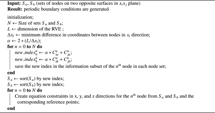
Periodic boundary condition generation algorithm for surface nodes

The process of generating periodic boundary condition constraints for the surface nodes is shown in Algorithm 1. In this algorithm, ${C}^{n}_{ia}$ and ${C}^{n}_{ib}$ are the coordinates i ($i=1,2,3$) of node n in sets $S_a$ and $S_b$, respectively. ${new\_index}^{n}_{k}$ is the new index of node n in set $S_k$ ($k=a,b$). It should be pointed out that the amplification factor, $\alpha$, only needs to be greater than the size of the RVE model divided by the minimum value of the coordinate difference of the nodes in the magnified direction. To choose $\alpha$, here we simply multiply this ratio by 2.

For nodes which are purely on the surface (i.e. not on the edges or vertices), we can directly apply an equation constraint. However, nodes on edges and vertices correspond to more than one opposite node, while it is not possible to apply more than one equation constraint to a node. To address this issue, nodes on the edges and vertices are applied a constraint one by one such that each node can appear only one time as the first node of the equation constraint.

2.3 Homogenization

Transfer of information between the micro and macro scales is one of the most important aspects of multiscale simulations. For this purpose, we use the periodic homogenization technique [63,64,65]. We define the equivalent stress at the macro-scale as

$$\begin{aligned} \varvec{\Sigma } = \frac{1}{V}\int _{V} \varvec{\sigma } \, \textrm{d}V \,. \end{aligned}$$

(6)

From Eqs. 2 and 3, the macroscopic strain $\varvec{E}$ is directly obtained as

$$\begin{aligned} \varvec{E} = \frac{1}{V}\int _{V} \varvec{\varepsilon } \, \textrm{d}V \,. \end{aligned}$$

(7)

For numerical implementation, we discretize the integrals in Eqs. 6 and 7 as

$$\begin{aligned} \varvec{\Sigma }= & \frac{1}{V}\sum _{i=0}^{N_{ip}}v_i\varvec{\sigma }_i \,, \end{aligned}$$

(8)

$$\begin{aligned} \varvec{E}= & \frac{1}{V}\sum _{i=0}^{N_{ip}}v_i\varvec{\varepsilon }_i \,, \end{aligned}$$

(9)

where $\varvec{\sigma }_i$ and $\varvec{\varepsilon }_i$ represent micro stress and strain tensors at the integration point i, respectively. $v_i$ is the volume of integration point i and $N_{ip}$ is the number of integration points in the RVE model. We use a postprocessing script (see Section Data availability) in ABAQUS CAE to get the simulation outputs (from ODB files) and calculate the macroscopic stress and strain from Eqs. 8 and 9.

2.4 Material properties

In this paper, we primarily focus on carbon fiber-reinforced metal matrix composites, which have extensive applications in aerospace, automotive industry and various other fields. Carbon fiber has the characteristics of high hardness, high strength, lightweight, high chemical resistance, high temperature resistance, and low thermal expansion, making it widely used in the field of aerospace. Aluminum alloys, e.g. 7075 aluminum alloy, are commonly used matrix materials for carbon fiber-reinforced composites in aerospace industry. Aluminum alloys have low density, good mechanical properties, good processing performance, nontoxicity, easy recycling, excellent conductivity, heat transfer, and corrosion resistance. They are widely used in the aerospace, marine industry, chemical industry, metal packaging, transportation, and other fields [66,67,68].

In this work, fibers are selected as intermediate modulus carbon fiber with Young’s modulus of 324 GPa, tensile strength of 7 GPa and Poisson’s ratio of 0.1. The matrix is selected to be 7075-T6 aluminum alloy, with Young’s modulus of 71.7 GPa, Poisson’s ratio of 0.33, and hardening modulus of 0.013. Fibers are assumed to be linearly elastic, and the matrix is modeled with J2 plasticity.

To demonstrate the applicability of our framework to other RVE behaviors, we also present numerical examples in which the material behavior of the matrix is modeled using Drucker-Prager plasticity. In these examples, for the matrix, the Young’s modulus, Poisson’s ratio, and hardening modulus are 324 GPa, 0.1, and 0.013, respectively. The angle of friction and dilation angle are both set to $45^\circ$, and the flow stress ratio is set to 1. The material model and parameters of the fibers remain unchanged.

3 Surrogate modeling

3.1 Data generation and sampling

Creating suitable training datasets is a crucial part of machine learning models, since it directly affects model quality and accuracy. The strain sampling algorithm is used to generate macroscopic strain series to be applied to the RVE for high-fidelity simulations. In a standard nonlinear FE boundary value problem, the strain series are not controlled or known a priori at integration points. Therefore, developing a strain sampling algorithm which performs well in general boundary value problems is essential [33].

Here we develop an algorithm inspired by random walks in a stochastic process and series selection. Random walk-based generation of training data provides generalization capability for trained models [33, 60]. Random strain increments (positive or negative) which are in a pre-defined range $(-\Delta E_{max},\Delta E_{max})$ are drawn from a uniform distribution to generate strain series independently for each strain component. Using the plasticity material model, the stress tensor at each step is calculated and the number of load steps which fall in the plastic range are determined for each series. If the number of plastic load steps in a series exceeds a given threshold ($M_p$), this series is stored in the dataset. The advantage of this algorithm is that it specifies the minimum number of plastic points in the series, which can give our GRU model sufficient information to learn the plastic behavior of the material. Algorithm 2 shows our proposed strain sampling procedure. An example strain series generated by this algorithm is illustrated in Fig. 3. Comparison of the proposed data generation scheme with other existing algorithms in the literature is provided in Sect. 5.1. The parameters used for data generation in this work are listed in Table 1.

Table 1 Parameters used for data generation

Algorithm 2

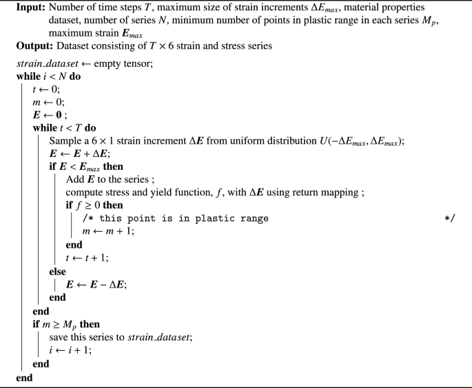
The proposed strain data generation scheme

Fig. 3

Example of strain series generated by Algorithm 2

The material properties generation script reads the material properties ranges of fiber and matrix from the preprocessing data generation script, and randomly generates material properties in the specified ranges. The geometry dataset generation script creates the data needed for an RVE model with multiple fibers randomly located in a matrix. This script randomly generates the coordinates of the fiber centers and checks the distances between fibers as well as between fibers and the edge of the RVE model to avoid overlap. If the generated coordinates cause overlaps, the code deletes and regenerates them, repeating the process until all fibers are created without overlap. In this work, we use the geometry shown in Fig. 2 to generate RVE models. Nevertheless, our preprocessing script is capable of generating RVE geometries with randomly distributed fibers.

3.2 Model architecture

Gated Recurrent Unit (GRU) is a variant of RNNs, which was developed to address the long-term dependency and vanishing gradient issues in the original RNN architecture. GRU has a gating mechanism that controls the flow of information through update and reset gates, and performs better for long series compared to the original RNN architecture. In this work, a GRU model is trained to learn the homogenized behavior of elasto-plastic composite RVE.

At each time step t, the input $\varvec{x}_t$ and the hidden state $\textbf{h}_{t-1}$ from the previous step are given to the GRU cell. Subsequently, the GRU cell calculates the updated hidden state $\textbf{h}_{t}$ and output $\textbf{y}_{t}$. The following calculations are done at each time step in the GRU cell:

$$\begin{aligned} \textbf{r}_{t}= & \sigma \left( \textbf{W}_{ir} \textbf{x}_{t} + \textbf{b}_{ir} + \textbf{W}_{hr} \textbf{h}_{t-1} + \textbf{b}_{hr}\right) \qquad \end{aligned}$$

(10)

$$\begin{aligned} \textbf{z}_{t}= & \sigma \left( \textbf{W}_{iz} \textbf{x}_{t} + \textbf{b}_{iz} + \textbf{W}_{hz} \textbf{h}_{t-1} + \textbf{b}_{hz}\right) \qquad \end{aligned}$$

(11)

$$\begin{aligned} \textbf{n}_{t}= & \tanh \left( \textbf{W}_{in} \textbf{x}_{t} + \textbf{b}_{in} + \textbf{r}_{t} * \left( \textbf{W}_{hn} \textbf{h}_{t-1} + \textbf{b}_{hn}\right) \right) \qquad \end{aligned}$$

(12)

$$\begin{aligned} \textbf{h}_{t}= & \left( \textbf{1} - \textbf{z}_{t}\right) * \textbf{n}_{t} + \textbf{z}_{t} * \textbf{h}_{t-1} \qquad \end{aligned}$$

(13)

$$\begin{aligned} \textbf{y}_{t}= & \textbf{W}_{hy} \textbf{h}_{t} + \textbf{b}_{y} \qquad \end{aligned}$$

(14)

in which $\textbf{r}_{t}$, $\textbf{z}_{t}$, and $\textbf{n}_{t}$ are the reset gate, update gate, and the candidate hidden state, respectively. $\sigma$ is the sigmoid function, and operator "$*$" denotes element-wise Hadamard multiplication. The GRU structure is illustrated in Fig. 4. The reset gate determines the amount of information from the previous steps which is discarded, while the update gate determines the amount of information retained from the previous steps to calculate the new hidden state. Finally, a linear layer maps the hidden state to the output. The architecture used in this work is illustrated in Fig. 5. In Fig. 5, $\textbf{E}_{t}$ (macroscopic strain tensor), $\textbf{h}_{t}$, and $\varvec{\hat{\Sigma }}_{t}$ (predicted macroscopic stress tensor) are the input, hidden state, and output, respectively. T is the number of time steps or the length of the series.

Fig. 4

Structure of a GRU cell

Fig. 5

The structure of our GRU based surrogate model

3.3 Training process

To train and test our GRU model, we divide 90% of the entire dataset into a training dataset and 10% into a test dataset. Since the components of strain and stress tensors have different magnitudes, we normalize the dataset before training to avoid convergence issues and model bias. For this purpose, we use the Min-Max scaler as follows:

$$\begin{aligned} {\Sigma '}_{i,k} = \frac{\Sigma _{i,k} - \Sigma _{\text {min}}}{\Sigma _{\text {max}} - \Sigma _{\text {min}}}, \quad {E'}_{i,k} = \frac{E_{i,k} - E_{\text {min}}}{E_{\text {max}} - E_{\text {min}}} \,, \end{aligned}$$

(15)

in which $\Sigma _{i,k}$ and $E_{i,k}$ denote component k of the ith original stress and strain data points, and $\Sigma '_{i,k}$ and $E'_{i,k}$ are their transformed versions. $\Sigma _{\text {min}}$ and $E_{\text {min}}$ are the minimum values of stress and strain, respectively, across all samples, time steps, and components in the dataset. $\Sigma _{\text {max}}$ and $E_{\text {max}}$ are the maximum values of stress and strain, respectively, across all samples and time steps in the dataset.

The model is trained using the PyTorch library. The mean squared error (MSE) is selected as the loss function:

$$\begin{aligned} \text {MSE} = \frac{1}{NT} \sum _{n=1}^{N} \sum _{t=1}^{T} \left\| \varvec{\Sigma }_{n,t} - \hat{\varvec{\Sigma }}_{n,t} \right\| _{2}^{2} \,, \end{aligned}$$

(16)

where $\varvec{\Sigma }_{n,t}$ and $\hat{\varvec{\Sigma }}_{n,t}$ denote the reference and predicted stress tensors of sample n at time step t. N and T are the total number of samples and time steps, respectively. The hyper-parameters used for training are shown in Table 2. In this work, we use the Adaptive Moment Estimation (Adam) algorithm to train our model.

Table 2 Hyper-parameters used for model training

To determine the optimal hyper-parameters of the model, we tune the individual hyper-parmaters one at a time based on the average mean squared error (MSE) on the test dataset. The learning rate decay mechanism is implemented, during which the learning rate is reduced by a factor. Hyper-parameter tuning is performed to obtain the optimal number of layers and hidden states, as shown in Table 3.

Table 3 Hyper-parameters used in the model architecture

Fig. 6 shows the training and test loss curves versus epochs. At the end of the training process, the training MSE is about $2.6 \times 10^{-7}$. Convergence of training and test loss is an indicator that the model is trained well. An example of the model performance on the test dataset is shown in Fig. 7 for all 6 stress and strain components. It is observed that the predicted values closely align with the true values across all six stress components.

Fig. 6

Training and testing loss curves versus epochs

Fig. 7

Comparison of the true and predicted macroscopic stress corresponding to a sample from the test dataset. The solid red line represents the true value (obtained from high-fidelity RVE simulations) and the blue dashed line represents the model prediction

It is important to note that training and test losses only help ensure the quality of training and assess the model performance on similar types of datasets. To fully validate our models and its robustness in multiscale FE simulations, multiple boundary value problems with unseen loading scenarios (which were not included in the training/testing datasets) are presented in Sect. 5.

4 Multiscale framework

We implement a $FE^{2}$ multiscale framework based on the trained GRU model. In the traditional $FE^{2}$ method, the strain obtained from the macroscopic finite element simulation is transferred to the microscopic scale to simulate the RVE model. Subsequently, the simulation result is homogenized and transferred to the macroscopic scale as macroscopic stress and stiffness tangent. For elasto-plastic materials, simulating high-fidelity RVE models at every iteration of the nonlinear solver is cumbersome. To address this problem, we use a trained GRU model to replace the microscopic full-field simulations of RVEs. For this purpose, we directly use the strain obtained at the macroscopic scale as input to the GRU model, and use the output of GRU as macroscopic stress in the macroscopic FE simulation.

In this work, we use the commercial software ABAQUS to implement this process, which has the capability to incorporate a user material subroutine (UMAT) for defining a user-defined constitutive relationship. We implement our trained GRU model in UMAT as the material model and use it in multiscale simulations. The following subsection describes our developed process for integrating a trained GRU model within UMAT, which we make accessible in a public repository (see Section Data availability).

4.1 Implementation of trained GRU models in UMAT

Here we develop a general FORTRAN algorithm for integrating trained GRU models within ABAQUS UMAT, as described in Algorithm 3. This subsection describes the details of this algorithm.

Our FORTRAN Algorithm 3 consists of three main parts. The first part defines subroutines frequently called in the subsequent sections of the code, including matrix operators, activation functions, the Min-Max scaler and its inverse. The second part implements the trained GRU model. First, the variables storing model parameters and temporary variables are declared. Due to the large number of model parameters, we provide a Python script to directly write the model parameters into the UMAT file. Subsequently, the model parameters, input vector, and hidden state vector are loaded. Finally, the GRU model is reconstructed layer by layer using the Basic Subroutines defined in Part 1.

In the final part, the UMAT interface is used by ABAQUS to call the UMAT subroutine. This part can be found in the documentation of ABAQUS and is immutable. In addition, the necessary variables that are not provided by the UMAT interface are declared. Subsequently, we compute the Jacobian matrix and call the Trained GRU Subroutine to calculate the output and hidden state vectors. In this work, we use the Quasi-Newton solver in ABAQUS, which eliminates the need to update the Jacobian matrix at each step and simplifies the implementation. Finally, the Min-Max Scaler Inverse Subroutine calculates the macroscopic stress vector.

Algorithm 3

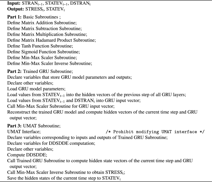
Implementation of trained GRU model in ABAQUS UMAT

In Algorithm 3, $\mathrm {STRAN_{t-1}}$ and $\mathrm {DSTRAN_{t}}$ represent the strain vector of the previous time step and the strain increment vector, respectively. DDSDDE represents the Jacobian matrix. $\mathrm {STRESS_{t}}$ is the stress vector at the end of the current time step. $\mathrm {STATEV_{t-1}}$ and $\mathrm {STATEV_{t}}$ represent the vectors of ABAQUS state variables corresponding to the previous and current time steps, respectively, with their length stored in ABAQUS variable “DEPVAR". In this work, we use these variables to store the hidden states $\textbf{h}_{t-1}$ and $\textbf{h}_{t}$ of the GRU model. Here the lengths of $\mathrm {STATEV_{t-1}}$ and $\mathrm {STATEV_{t}}$ are equal to the sum of the lengths of the hidden state vectors of all GRU layers.

The above steps provide the template of the GRU-UMAT code without specified parameters. We have designed a Python script to traverse each line of the UMAT file and write the model parameters in appropriate locations. The final UMAT script is saved as a FORTRAN file to be called during macroscopic FE simulations in ABAQUS.

5 Results

In the numerical examples of this section, we assume that our RVE is a cube with a single fiber in the center of the RVE model, as shown in Fig. 2. We set the dimension of the RVE to 1 and the radius of the fiber to 0.35. Mesh size used for RVE simulations is 0.075. The parameters used for data generation and the GRU model are listed in Tables 1, 2, 3. While we use the geometry shown in Fig. 2 to generate RVE models for model training and performing the numerical examples, our framework and preprocessing script are applicable to RVE geometries with randomly distributed fibers. For this purpose, the GRU model can be generalized to other geometries by including geometrical descriptors such as the number of fibers and their diameters as model input.

To compare the results of our model with reference solutions, we use the following formula for computing the relative error:

$$\begin{aligned} E(\varvec{\hat{\Sigma }})= & \frac{ {\parallel \varvec{\hat{\Sigma }} - \varvec{\Sigma }_{ref}\parallel }_2 }{ {\parallel \varvec{\Sigma }_{ref}\parallel }_2 } , \end{aligned}$$

(17a)

$$\begin{aligned} E(\varvec{\hat{U}})= & \frac{ {\parallel \varvec{\hat{U}} - \varvec{U}_{ref}\parallel }_2 }{ {\parallel \varvec{U}_{ref}\parallel }_2 } , \end{aligned}$$

(17b)

$$\begin{aligned} E(\varvec{\hat{RF}})= & \frac{ {\parallel \varvec{\hat{RF}} - {\varvec{R}}{\varvec{F}}_{ref}\parallel }_2 }{ {\parallel \varvec{RF}_{ref}\parallel }_2 } , \end{aligned}$$

(17c)

in which $E(\varvec{\hat{\Sigma }})$, $E(\varvec{\hat{U}})$, and $E(\varvec{\hat{RF}})$ are the relative errors in stress, displacement and reaction force, respectively. $\varvec{\hat{\Sigma }}$, $\varvec{\hat{U}}$, and $\varvec{\hat{RF}}$ are the predicted vector series (for all time steps) for stress, displacement, and reaction force, while $\varvec{\Sigma }_{ref}$, $\varvec{U}_{ref}$, and $\varvec{RF}_{ref}$ are the corresponding reference values. The following error metric is utilized to obtain the error contour plots for displacements:

$$\begin{aligned} E({\hat{U_i}}) = \frac{ {|{\hat{U_i}} - {U}_{ref,i}|} }{ {\text {max}|{U}_{ref,i}|} } , \end{aligned}$$

(18)

in which $\hat{U_i}$ and ${U}_{ref,i}$ are the predicted and reference values of the ith component of the displacement vector, respectively. “$\text {max}$” operator returns the maximum value of each displacement component separately in the entire domain. This normalized metric is selected to avoid denominators that are close to zero when calculating relative errors.

5.1 Testing the new sampling algorithm

In general, performance of data generation algorithms depends on the machine learning model architecture; therefore, the best-performing sampling algorithms need to be designed and tested for each architecture [33]. To assess the performance of the data generation algorithm proposed in this work, we compare it with sampling algorithms developed in the literature [31, 33]. We apply the interpolation based sampling scheme in [31], the random walk based Algorithm 2 in [33] and our proposed Algorithm 1 to generate three datasets with 10, 000 samples each, with the same RVE and material properties described in Sect. 2.4 and Table 1.

We use linear cyclic strain loading protocols to test the model trained with each data generation algorithm. The loading protocol consists of 100 time steps, which starts from zero strain and changes the loading direction after every 25 steps while absolute value of the strain increment is constant. For example, the strain component starts at 0, increases from step 1 to step 25, then decreases from step 26 to step 75, and finally increases back to 0 from step 76 to step 100. The initial increments of axial and shear strain components are $\pm 0.0004$ and $\pm 0.0001$, respectively. In addition, signs of 6 strain components are varied such that there are $2^6=64$ testing protocols corresponding to each strain increment case.

50 random scaling factors are drawn from a uniform distribution between 0.75 and 5. The range of scaling factors is selected such that the material can still enter the plastic range. These scaling factors are multiplied by the aforementioned 64 testing protocols, leading to 3200 sample test series with varying absolute values of strain increments. The average of relative errors (Eq. 17a) obtained from GRU models trained using data generated with different sampling algorithms are calculated based on these 3200 test samples, and subsequently plotted against the maximum strain increment size of test samples in Fig. 8. It is observed that our proposed Algorithm 1 produces the smallest errors across all strain increment sizes.

Fig. 8

Comparison of relative errors versus strain increment size obtained from our new sampling algorithm and the reference algorithms

5.2 Test in microscale problems

In this example, we test the performance of our model in response to loading protocols not included in the training and test datasets. Four loading protocols are designed for macroscopic strain, namely, monotonic (Fig. 9a), linear cyclic with zero shear strains (Fig. 9b), linear cyclic with non-zero shear strain (Fig. 9c), and sinusoidal cyclic (Fig. 9d) protocols. We use these loading protocols for macroscopic strain to perform high-fidelity simulations of the RVE, calculate homogenized macroscopic stresses, and use them as true (reference) value. Specifically, we use our preprocessing code to apply the generated macroscopic strain series to the RVE model with periodic boundary conditions and run the full-field simulations. The postprocessing and homogenization scripts are used to compute the homogenized stress of this RVE as the reference value. The predicted values are obtained from our GRU model with the given macroscopic strain series as input.

Fig. 9

Four strain loading protocols used for model validation: a monotonic load with zero shear strains, b linear cyclic load with zero shear strains, c linear cyclic load with non-zero shear strains, and d sinusoidal load with zero shear strains

In the monotonic case, (Fig. 9a), $E_{11}$ and $E_{22}$ are monotonically decreasing from 0 to $-$0.01 with fixed increments of $-$0.0002. $E_{33}$ monotonically increases from 0 to 0.02 with fixed increments of 0.0004, and $E_{12}=E_{13}=E_{23}=0$. The number of time steps is equal to 50. The performance of our model for J2 plasticity is illustrated in Fig. 10 for all components of stress, and relative error in this case is 0.00485.

Fig. 10

The predicted and true stresses versus time steps corresponding to the monotonic strain loading protocol shown in Fig. 9a for J2 plasticity

For the linear cyclic protocol with zero shear strains (Fig. 9b), the peak value and fixed increment size of $E_{11}$ and $E_{22}$ are ±0.005 and ±0.0002 respectively, while the peak value and fixed increment size of $E_{33}$ are ±0.01 and ±0.0004 respectively. The number of time steps is equal to 100. Figures 11 and 12 show the stress time history and stress versus strain behavior of the GRU model for J2 plasticity. The relative error in this case is 0.0147.

Fig. 11

The predicted and true stresses versus time steps corresponding to the linear cyclic strain loading protocol shown in Fig. 9b for J2 plasticity

Fig. 12

The predicted and true stress versus strain plots corresponding to the linear cyclic strain loading protocol shown in Fig. 9b for J2 plasticity

In the case of linear cyclic protocol with non-zero shear strains (Fig. 9c), the number of time steps is equal to 100. The peak value and fixed increment of $E_{11}$ and $E_{22}$ are ±0.005 and ±0.0002, and the peak value and fixed increment of $E_{33}$ are ±0.01 and ±0.0004, respectively. The increments of shear strain components are $\Delta E_{12} = 0.0001$, $\Delta E_{13}=-0.0001$, and $\Delta E_{23} = 0.000075$. Figures 13 and  14 show the stress time history and stress versus strain behavior of the GRU model for J2 plasticity. The relative error in this case is 0.0152. Figures 15 and 16 show the stress time history and stress versus strain behavior of the GRU model for Drucker-Prager plasticity. The relative error in this case is 0.039.

Fig. 13

The predicted and true stresses versus time steps corresponding to the linear cyclic strain loading with non-zero shear strain protocol shown in Fig. 9c for J2 plasticity

Fig. 14

The predicted and true stress versus strain plots corresponding to the linear cyclic strain loading protocol with non-zero shear strain shown in Fig. 9c for J2 plasticity

Fig. 15

The predicted and true stresses versus time steps corresponding to the linear cyclic strain loading protocol shown in Fig. 9c for Drucker-Prager

Fig. 16

The predicted and true stress versus strain plots corresponding to the linear cyclic strain loading protocol shown in Fig. 9c for Drucker-Prager

The sinusoidal loading case has zero shear strains (Fig. 9d), the peak value of $E_{11}$ and $E_{22}$ is ±0.005, and the peak value of $E_{33}$ is ±0.01. However, the strain increments are not constant, and the strain series has 100 time steps. Figures 17 and 18 show the model performance in predicting stresses for J2 plasticity with a relative error of 0.0250.

Fig. 17

The predicted and true stresses versus time steps corresponding to the sinusoidal cyclic strain loading protocol shown in Fig. 9d for J2 plasticity

Fig. 18

The predicted and true stress versus strain plots corresponding to the sinusoidal cyclic strain loading protocol shown in Fig. 9d for J2 plasticity

It is observed from Figs. 10 to 18 that the GRU model predictions follow the results of high-fidelity simulations very closely for all loading protocols. The loading patterns used here are considered difficult for the model since they were not included in the training set. Nevertheless, the model produces small relative errors. In loading cases with zero shear strains, the model correctly predicts zero shear stresses. Overall, the axial components obtained from the GRU model almost completely match the high-fidelity solutions, while the model is less accurate in predicting shear components due to their smaller magnitudes.

5.3 Test in multiscale boundary value problems

Through testing at the microscale in subsection 5.2, we have validated the performance of our GRU model at the microscale under given macroscopic strain states. In this subsection, we reconstruct the trained GRU model in ABAQUS UMAT and use it to perform 3D multiscale finite element simulations to verify the effectiveness of our model in practical scenarios. The multiscale problems in this section are fundamental, including a 3D bar in tension, cantilever beam bending, tensile test on a coupon with imperfection, and a square plate with a hole. Various loading patterns (cyclic, monotonic, force driven, and displacement driven) are applied to thoroughly test the capability of the model to perform well in multiscale settings.

In each example, two sets of simulations are performed. First, the high-fidelity geometry of the boundary value problem is generated with fully resolved microstructure, and high-fidelity traditional finite element simulations are performed with fine mesh to serve as the reference solution. In these simulations, the built-in material models in ABAQUS are directly used to create material properties of the fibers and matrix. The second set of simulations consist of the macroscopic geometric structure of the boundary value problems (that is, without modeling the microstructural features explicitly), in which our GRU-based UMAT code (see Sect. 4.1) is used as the material subroutine to represent the material behavior at integration points. In this case, simulations are performed with coarse mesh. Finally, we compare the results of these two sets of simulations to assess the accuracy of our GRU-based model.

We take l and L to represent the dimension of the RVE model and the shortest length of the cross-section perpendicular to the fiber direction in the high-fidelity model, respectively. In this section, we use two different values of $l/L=0.25$ and $l/L=0.1$ for the high-fidelity models. In the following examples, we plot and compare the maximum absolute value of displacement of each group of test results. $U_1$, $U_2$ and $U_3$ denote displacements in the x (or $x_1$), y (or $x_2$) and z (or $x_3$) directions, respectively. We use ParaView to generate contour plots of our simulations. Shen et al. [69] developed a software that can transform ABAQUS output ODB files to VTU for visualization in ParaView, which is used in this work.

5.3.1 Example 1: Tensile test on a 3D bar

In this example, we examine the performance of our trained GRU model in uniaxial tension of a 3D composite beam. Consider a 3D beam as illustrated in Fig. 19a, where the fibers are shown in green. The length of this beam is equal to 5, while the width and height of the cross-section are equal to 1. Fibers are oriented along the beam axis, that is, the z (or $x_3$) direction.

The boundary conditions are illustrated in Fig. 19b. A surface traction with magnitude of 1600 MPa is applied to one surface of the beam along the z direction. In addition, we use a coupling constraint on the z-positive plane to keep all nodes on this surface flat. The number of time steps is equal to 50. The displacements of the other end of the beam are fixed in the z direction and appropriate boundary conditions are set to prevent rigid body motion. In the high-fidelity simulations, a fine mesh with mesh size equal to 0.05 (for $l/L=0.25$) and 0.02 (for $l/L=0.1$) is used, while the macroscopic simulation is performed with a coarse mesh of size 0.5.

Fig. 19

a The geometry and b boundary condition of the cantilever beam in the tensile test

The displacement distributions in the z-direction of high-fidelity simulations are illustrated in Figs. 20a and b for $l/L=0.25$ and $l/L=0.1$, respectively. The displacement distribution in the z-direction of multiscale simulation is illustrated in Fig. 20c. The relative errors (Eq. 17b) of maximum displacements are 0.0277 and 0.0279 when $l/L=0.25$ and $l/L=0.1$, respectively. Fig. 21 compares the maximum axial displacement versus the applied load of the reference (high-fidelity) simulation and our GRU-based multiscale simulation. It is observed that even though a coarse mesh is used for GRU-based multiscale simulations, the displacement field and overall response of the bar match the high-fidelity simulations with a much finer mesh.

In addition, we select element “A” (marked in Fig. 20c), and extract stress and strain time history data at integration point 1 of this element. The stress data from this integration point is predicted by the GRU model. Meanwhile, we use the extracted strain data to perform high-fidelity RVE simulations and homogenization to obtain the reference value of macroscopic stress. Fig. 22 shows the predicted and reference stress components. It is observed that the predicted response of our model matches the reference solution very well, with a small relative error of 0.0125.

Fig. 20

Comparison of the displacement fields obtained from high-fidelity and multiscale simulations of a 3D bar in tension

Fig. 21

Maximum displacement in the z (axial) direction versus the load applied to the bar in tension

Fig. 22

The true and predicted stress values at integration point “A" versus time steps in the 3D bar in tension

5.3.2 Example 2: Cantilever beam bending test

Consider a 3D composite beam with the same geometry as Example 1 (Sect. 5.3.1) and boundary conditions shown in Fig. 23. One side of the beam is subjected to surface traction of 100 MPa along the y-negative direction, while all displacement degrees of freedom are fixed at the other end of the beam. Mesh sizes of 0.05 (for $l/L=0.25$) and 0.02 (for $l/L=0.1$) are selected for the high-fidelity simulations, while the macroscopic simulation is performed with a coarse mesh of size 0.25. Figure 24 compares the distribution of displacements in the y-direction of high-fidelity simulations with the GRU-based multiscale simulation. It is observed that even though a coarse mesh is used for GRU-based multiscale simulations, the displacement field and overall response of the beam are close to the high-fidelity simulations with a much finer mesh.

Fig. 23

The boundary conditions of the 3D cantilever beam bending test

Figure 25a compares the maximum displacement in the y-direction ($U_2$) obtained from the reference and GRU-based multiscale simulations versus the load applied to the cantilever beam. The relative errors in maximum displacement are 0.0549 and 0.0221 calculated using high-fidelity simulations with $l/L=0.25$ and $l/L=0.1$, respectively.

Fig. 24

Comparison of the displacement fields of high-fidelity and multiscale simulations of the cantilever beam bending test

Stress and strain time history data during GRU-based multiscale simulations are extracted at integration point 1 of element "A" marked in Fig. 24c. The stress value is predicted by the GRU model. Meanwhile, we use strain data to perform high-fidelity simulation and homogenization on the RVE to obtain the reference value of stress. It is observed from Fig. 26 that the reference and predicted stress values are very close, and the relative error (Eq. 17a) is calculated as 0.020.

Fig. 25

The maximum displacement in the y-direction versus the load applied in the cantilever beam bending test

Fig. 26

The reference and predicted stress components versus time steps at integration point "A" in the cantilever beam bending test

5.3.3 Example 3: Tensile test of coupon with imperfection

In this example, we consider a coupon with two semi-circular openings on both sides at the midpoint of the coupon, each with a radius of 0.25. The geometry and boundary conditions are illustrated in Fig. 27. One end of the coupon is subjected to surface traction of 600 MPa along the z-positive direction, while the displacements of the other end of the beam are set to zero in the z direction and appropriate boundary conditions are set to prevent rigid body motion. We also set a coupling constraint on the z-positive plane to keep all nodes on this surface flat. We use tetrahedral mesh of size 0.1 for the high-fidelity simulation, while the multiscale simulation is performed with hexahedral mesh of size 0.15.

Fig. 27

Boundary conditions of the coupon tensile test

The distribution of displacements in the z direction obtained from high-fidelity and multiscale simulations match very well, as illustrated in Fig. 28a and b, respectively. The contour plots of von Mises stress and von Mises strain of multiscale simulation of this problem are illustrated in Fig. 29a and b, respectively. It is observed that our GRU-based multiscale model successfully predicts the stress and strain concentration around the imperfection.

Fig. 28

Comparison of displacement fields of high-fidelity and multiscale simulations of the coupon tensile test

Fig. 29

Von Mises stress and strain fields in multiscale simulation of the coupon tensile test

Fig. 30 compares the maximum displacement in the z direction versus the applied load obtained from the reference and GRU-based multiscale simulations. The relative error (Eq. 17b) of maximum displacement between the two simulations is 0.053. We extract the historical strain and stress data of integration point 1 of element "A" shown in Fig. 28b. Figure 31 shows that stress components obtained from the reference solution and our GRU model at this integration point match well, with a relative error of 0.0145.

Fig. 30

The maximum displacement in the z direction versus the traction applied to the coupon

Fig. 31

The reference and predicted stress components versus time steps at integration point "A" of the coupon tensile test

5.3.4 Example 4: Perforated square plate under linear cyclic load

In this section, we test a fiber composite thick plate with a circular hole in its center, as illustrated in Fig. 32. Due to symmetry, only one quarter of the domain is modeled. The length and width of this thick plate are both 4, with a thickness of 1. The circular perforation has a radius of 1 and is located at the center of this plate, with the direction of perforation perpendicular to the direction of fiber extension. The fibers are along the z (or $x_3$) direction. Surface traction of $\pm {200}$ MPa is applied along the y direction on the top surface of the plate, following a cyclic pattern similar to the protocol of ${E}_{33}$ in Fig. 9b. The number of time steps is equal to 100. In this problem, we use fine tetrahedral mesh of size 0.1 for the high-fidelity simulation, and hexahedral mesh of size 0.15 for the multiscale model.

Fig. 32

Geometry of the thick plate with a circular perforation: a 2D plane projection of the thick composite plate model, b 3D model of the one-quarter part of the thick plate

Fig. 33

Mesh used for multiscale simulation of the square plate. Elements and nodes used to probe stress–strain and displacement data are marked

Figure 34 and 35 show the distribution of displacements in y and z directions, respectively, obtained from high-fidelity and multiscale simulations in the 75th time step corresponding to the minimum loading step. For $l/L=0.25$, the relative errors of maximum displacement in y and z directions are 0.0093 and 0.012, respectively. For $l/L=0.1$, the relative errors of maximum displacement in y and z directions are 0.032 and 0.067, respectively. The distributions of von Mises stress and von Mises strain obtained at the 75th time step of the multiscale simulation are shown in Fig. 36a and b, respectively. It is observed that the GRU-based model is capable of capturing concentration of stress and strain around the circular hole. Error distributions of the displacement field in y and z directions are shown in Figs. 34d and 35d obtained using the error metric in Eq. 18. We observe that the errors are generally small in the domain and do not exceed about 10% and 6% in the z and y directions, respectively. We note that the error metric in Eq. 18 is essentially a normalized measure of the absolute error as opposed to the relative error. Therefore, regions with larger magnitudes of displacements may be expected to show larger errors.

Fig. 34

Example 4: Distribution of displacements in the y direction of a high-fidelity simulation ($l/L=0.25$), b high-fidelity simulation ($l/L=0.1$), and c GRU-based multiscale simulation at the 75th time step under linear cyclic surface traction force. d Error distribution plot of displacements in the y direction

Fig. 35

Example 4: Distribution of displacements in the z direction of a high-fidelity simulation ($l/L=0.25$), b high-fidelity simulation ($l/L=0.1$), and c GRU-based multiscale simulation at the 75th time step under linear cyclic surface traction force. d Error distribution plot of displacements in the z direction

Fig. 36

Example 4: a von Mises stress and b von Mises strain distribution of multiscale simulation at the 75th time step under linear cyclic load

A few nodes and elements of interest are marked on Fig. 33. Displacement in the y direction at node “a” and displacement in the z direction of node “b” are plotted against the traction applied to the plate in Fig. 37. For $l/L=0.25$ and $l/L=0.1$, the relative error of $U_2$ is 0.066 and 0.070, respectively. According to the position of stress concentration, we select integration point 7 of element “C” to plot the reference and predicted stress time histories, as shown in Fig. 38. The relative error of our GRU model at this integration point is 0.051.

Fig. 37

Example 4: a Displacement in y direction of node “a”, and b displacement in z direction of node “b” versus the applied surface traction for the quarter square plate problem under linear cyclic load

Fig. 38

Example 4: Reference and predicted stress components at integration point 7 of element C versus time steps

5.3.5 Example 5: Perforated square plate under cyclic displacement

In this example, we consider the same quarter plate problem shown in Fig. 32. Instead of a surface traction, the top surface of the plate is subjected to a cyclic uniform displacement along the y direction with the magnitude of $\pm {0.01}$ and a pattern similar to the protocol of ${E}_{33}$ in Fig. 9b. The number of time steps is set to 100. We use the same mesh as Example 4 (Sect. 5.3.4).

Fig. 39

Example 5: a von Mises stress and b von Mises strain distribution of multiscale simulation at the 75th time step under cyclic displacement

Figure 39 shows the distribution of von Mises stress and strains at the 75th time step of the GRU-based multiscale simulation. It is observed that the localized strain and stress are captured by the model. The total reaction force at the top surface versus the controlled displacement of the top surface is plotted in Fig. 40. The relative error of the prediction (Eq. 17c) is 0.082. We select integration point 8 of element “D” (marked in Fig. 39a) which is located in a stress localization zone to plot the reference and predicted stress components, as illustrated in Fig. 41. The relative error (Eq. 17a) of our GRU model at this integration point is about 10%.

Fig. 40

The total vertical reaction forces versus controlled top displacement

Fig. 41

Example 5: Reference and predicted stress components at integration point 8 of element “D" versus time steps

5.3.6 Example 6: Perforated square plate under sinusoidal load

In this subsection, we aim to test the model performance under more complex nonlinear loading. We consider the same square plate as Example 4, with boundary conditions shown in Fig. 32a. The upper surface of the plate is subjected to surface traction of magnitude $\pm {200}$ MPa along the y direction, with a pattern similar to the protocol of ${E}_{33}$ in Fig. 9d. We use the same mesh as Example 4 (Sect. 5.3.4).

Figures 42 and 43 show the displacement distributions in y and z directions, respectively, at the 75th time step of simulations. Despite using a coarser mesh in multiscale simulations compared to the high-fidelity simulations, the displacement distributions are captured well by our multiscale model. The relative errors in maximum $U_2$ and $U_3$ are 0.0122 and 0.0324, respectively, for $l/L=0.25$. For the case of $l/L=0.1$, relative errors in maximum $U_2$ and $U_3$ are obtained as 0.055 and 0.083, respectively. Error distributions of the displacement field in y and z directions are shown in Figs. 42d and 43d obtained using the error metric in Eq. 18. We observe that the errors are generally small in the domain and do not exceed about 7-11%. We note the errors are very small in most of the domain and concentrate around the regions where the displacement magnitudes are larger. This is due to the fact that the error metric in Eq. 18 is a normalized measure of absolute error, not the relative error. The distribution of von Mises stress and von Mises strain obtained at the 75th time step of multiscale simulation are shown in Figs. 44a and 44b, respectively, showing that the concentration of stress and strain around the circular hole is captured by the GRU-based multiscale model.

Fig. 42

Example 6: Comparison of the displacement distribution in y direction for a high-fidelity simulation with $l/L=0.25$, b high-fidelity simulation with $l/L=0.1$, and c multiscale simulation at the 75th time step under sinusoidal cyclic load. d Error distribution plot of the displacement in y direction

Fig. 43

Example 6: Comparison of the displacement distribution in z direction for a high-fidelity simulation with $l/L=0.25$, b high-fidelity simulation with $l/L=0.1$, and c multiscale simulation at the 75th time step under sinusoidal cyclic load. d Error distribution plot of the displacement in z direction

Fig. 44

Example 6: a von Mises stress and b von Mises strain distribution of multiscale simulation at the 75th time step

The plots of $U_2$ at node "a" and $U_3$ at node "b" versus the applied load on the plate are shown in Fig. 45. The relative errors of $U_2$ are 0.092 and 0.076 for $l/L=0.25$ and 0.1, respectively. Time histories of reference and predicted stress components at integration point 7 of element "C" (marked in Fig. 33) are plotted in Fig. 46. The relative error of our GRU model at this integration point is 0.045, which is even better than the linear case. This test demonstrates that the performance of our model is similar to the linear case.

Fig. 45

Example 6: a Displacement in y direction of node “a”, and b displacement in z direction of node “b” versus the applied surface traction for the quarter square plate problem under sinusoidal cyclic load

Fig. 46

Example 6: Reference stresses at integration point 7 of element C versus time steps (sinusoidal surface traction force)

5.3.7 Example 7: Perforated square plate with Drucker-Prager matrix under linear cyclic load

In this subsection, we aim to test the model performance for Drucker-Prager material behavior. We consider the same square plate as Example 4, with same geometry, boundary conditions and mesh, but with Drucker-Prager material behavior for the matrix instead of J2 plasticity. The material parameters are defined in Sect. 2.4. The upper surface of the plate is subjected to surface traction of magnitude $\pm {150}$ MPa along the y direction, with a pattern similar to the protocol of ${E}_{33}$ in Fig. 9d.

Figures 47 and 48 show the distribution of displacements in y and z directions, respectively, obtained from high-fidelity and multiscale simulations at the 75th time step which corresponds to the minimum loading step. For $l/L=0.25$, the relative errors of maximum displacement in y and z directions are 0.0095 and 0.035, respectively. For $l/L=0.1$, the relative errors of maximum displacements in y and z directions are 0.0053 and 0.035, respectively. The distribution of von Mises stress and von Mises strain obtained at the 75th time step of multiscale simulation are shown in Fig. 49a and b, respectively. We observe that the GRU-based multiscale model is capable of capturing concentration of stress and strain around the circular hole. Error distributions of the displacement field in y and z directions are shown in Figs. 47d and 48d obtained using the error metric in Eq. 18. We observe that the errors are generally small in the domain and are less than about 2-4%.

Fig. 47

Example 7: Distribution of displacements in the y direction corresponding to the perforated quarter plate with Drucker-Prager matrix: a high-fidelity simulation ($l/L=0.25$), b high-fidelity simulation ($l/L=0.1$), and c GRU-based multiscale simulation at the 75th time step under cyclic surface traction force. d Error distribution plot of displacement in the y direction

Fig. 48

Example 7: Distribution of displacements in the z direction corresponding to the perforated quarter plate with Drucker-Prager matrix: a high-fidelity simulation ($l/L=0.25$), b high-fidelity simulation ($l/L=0.1$), and c GRU-based multiscale simulation at the 75th time step under cyclic surface traction force. d Error distribution plot of displacement in the z direction

Fig. 49

Example 7: a von Mises stress and b von Mises strain distribution at the 75th time step under linear cyclic load, corresponding to multiscale simulation of the perforated quarter plate with Drucker-Prager matrix

A few nodes and elements of interest are marked on Fig. 33. Displacement in the y direction at node “a” and displacement in the z direction of node “b” are plotted against the traction applied to the plate in Fig. 50. For $l/L=0.25$ and $l/L=0.1$, the relative error of $U_2$ is 0.062 and 0.032, respectively. According to the position of stress concentration, we select integration point 3 of element “C” to plot the reference and predicted stress time histories, as shown in Fig. 51. The relative error of our GRU model at this integration point is 0.051.

Fig. 50

Example 7: a Displacement in y direction of node “a”, and b displacement in z direction of node “b” versus the applied surface traction for the Drucker-Prager quarter square plate problem under linear cyclic load

Fig. 51

Example 7: Reference and predicted stress components versus time steps at integration point 3 of element C in the Drucker-Prager quarter square plate problem under linear cyclic load

5.4 Testing in a 2D problem

In this work, our GRU model was trained using 3D data. In this section, we verify the robustness of this model in 2D. For this purpose, we consider a two-dimensional plane strain composite plate. The geometry and boundary conditions of the problem are illustrated in Fig. 52. Additional constraints are imposed to ensure that the displacements of all nodes on the upper surface are equal in the y direction. A similar constraint is imposed on the nodes located on the bottom surface. A uniform cyclic displacement is applied to the right surface of the plate along the x direction with a magnitude of $\pm {0.006}$ with a cyclic pattern similar to the protocol of ${E}_{33}$ in Fig. 9b. The number of time steps is equal to 100. In this problem, hybrid plane strain elements are used to perform high-fidelity and multiscale simulations. Fine mesh is needed for high-fidelity simulations. Therefore, the mesh size is set to 0.025, 0.01, 0.005, and 0.0025 for $l/L=0.25$, 0.1, 0.05 and 0.025, respectively. In the case of multiscale simulation, we use a coarse mesh with size 0.25.

Fig. 52

2D problem geometry and boundary conditions corresponding to $l/L = 0.1$

Figure 53 shows the plots of reaction force on the right surface of the 2D plate versus controlled displacement ${U}_{1}$ for $l/L=0.25$, 0.1, 0.05 and 0.025. The relative error in the 75th time step is 0.067 for $l/L=0.25$. It can be observed that the predictions obtained from the GRU-based multiscale model follow the high-fidelity simulation results well for all characteristic length ratios.

Fig. 53

Reaction force versus controlled displacement in x direction on the right surface of the 2D plate corresponding to characteristic lengths a $l/L=0.25$, b $l/L=0.1$, c $l/L=0.20$, and d $l/L=0.02$

6 Conclusion

Recently, Recurrent Neural Networks have shown promise for modeling the dissipative behavior of materials. However, widespread application of these techniques in multiscale finite element analysis has been hindered by challenges including: (1) input strains are dictated by the nonlinear FE solver which vary at each iteration and are not known a priori during the offline training stage, leading to poor model performance and convergence issues; and (2) there is a need for linking the trained machine learning models with existing widely used FE software packages.

In this work, we developed a 3D multiscale FE framework based on Gated Recurrent Units for long fiber composite materials and made it accessible through a public repository. We proposed a random walk-based sampling algorithm with series selection to achieve more effective data sampling, leading to a trained GRU model that shows higher accuracy compared to reference algorithms in response to different strain increment sizes used as input, thus performing effectively when implemented within a nonlinear FE solver. We developed a preprocessing script to generate the full-field FE models of the RVEs, and proposed an efficient algorithm to apply periodic boundary conditions to the RVE model through coordinate transformation and sorting. We developed a FORTRAN algorithm to reconstruct our trained GRU model in ABAQUS UMAT as a surrogate model (metamodel) to perform multiscale FE simulations.

We tested the performance of our surrogate model in RVE-level simulations and various 2D and 3D multiscale problems under monotonic, cyclic, and sinusoidal loading which were all unseen during the training process. We observed from the test results and comparison with high-fidelity simulations that the model captures time history of the overall structural response as well as evolution and distribution of field variables well, and consistently achieves small relative errors. We have provided the code in a public repository to make application of trained machine learning surrogate models for multiscale simulations in FE software more accessible and easy to adopt by users (Table 4).

Table 4 Meta data of our code

References

Kanouté P, Boso D, Chaboche J-L, Schrefler B (2009) Multiscale methods for composites: a review. Arch Comput Methods Eng 16:31–75. https://doi.org/10.1007/s11831-008-9028-8
Fish J, Wagner GJ, Keten S (2021) Mesoscopic and multiscale modelling in materials. Nat Mater 20(6):774–786. https://doi.org/10.1038/s41563-020-00913-0
Feyel F, Chaboche J-L (2000) Fe2 multiscale approach for modelling the elastoviscoplastic behaviour of long fibre SiC/Ti composite materials. Comput Methods Appl Mech Eng 183(3–4):309–330. https://doi.org/10.1016/S0045-7825(99)00224-8
Logarzo HJ, Capuano G, Rimoli JJ (2021) Smart constitutive laws: inelastic homogenization through machine learning. Comput Methods Appl Mech Eng 373:113482. https://doi.org/10.1016/j.cma.2020.113482
Xu R, Yang J, Yan W, Huang Q, Giunta G, Belouettar S, Zahrouni H, Zineb TB, Hu H (2020) Data-driven multiscale finite element method: from concurrence to separation. Comput Methods Appl Mech Eng 363:112893
Kim S, Shin H (2024) Data-driven multiscale finite-element method using deep neural network combined with proper orthogonal decomposition. Eng Comput 40(1):661–675
Bishara D, Xie Y, Liu WK, Li S (2023) A state-of-the-art review on machine learning-based multiscale modeling, simulation, homogenization and design of materials. Arch Comput Methods Eng 30(1):191–222. https://doi.org/10.1007/s11831-022-09795-8
Bock FE, Aydin RC, Cyron CJ, Huber N, Kalidindi SR, Klusemann B (2019) A review of the application of machine learning and data mining approaches in continuum materials mechanics. Front Mater 6:110. https://doi.org/10.3389/fmats.2019.00110
Liu X, Tian S, Tao F, Yu W (2021) A review of artificial neural networks in the constitutive modeling of composite materials. Compos B Eng 224:109152. https://doi.org/10.1016/j.compositesb.2021.109152 (https://www.sciencedirect.com/science/article/pii/S1359836821005321)
Ali U, Muhammad W, Brahme A, Skiba O, Inal K (2019) Application of artificial neural networks in micromechanics for polycrystalline metals. Int J Plast 120:205–219. https://doi.org/10.1016/j.ijplas.2019.05.001
Im S, Kim H, Kim W, Cho M (2021) Neural network constitutive model for crystal structures. Comput Mech 67:185–206. https://doi.org/10.1007/s00466-020-01927-w
Jang DP, Fazily P, Yoon JW (2021) Machine learning-based constitutive model for J2-plasticity. Int J Plast 138:102919. https://doi.org/10.1016/j.ijplas.2020.102919
Furukawa T, Yagawa G (1998) Implicit constitutive modelling for viscoplasticity using neural networks. Int J Numer Meth Eng 43(2):195–219. https://doi.org/10.1002/(SICI)1097-0207(19980930)43:2<195::AID-NME418>3.0.CO;2-6
Benabou L (2021) Implementation of a neural network into a user-material subroutine for finite element simulation of material viscoplasticity. J Eng Mater Technol 143(4):041001. https://doi.org/10.1115/1.4050704
Jung S, Ghaboussi J (2006) Neural network constitutive model for rate-dependent materials. Comput Struct 84(15–16):955–963. https://doi.org/10.1016/j.compstruc.2006.02.015
Jung S, Ghaboussi J (2006) Characterizing rate-dependent material behaviors in self-learning simulation. Comput Methods Appl Mech Eng 196(1–3):608–619. https://doi.org/10.1016/j.cma.2006.06.006
Li X, Roth CC, Mohr D (2019) Machine-learning based temperature-and rate-dependent plasticity model: Application to analysis of fracture experiments on dp steel. Int J Plast 118:320–344. https://doi.org/10.1016/j.ijplas.2019.02.012
Bhaduri A, Gupta A, Graham-Brady L (2022) Stress field prediction in fiber-reinforced composite materials using a deep learning approach. Compos B Eng 238:109879. https://doi.org/10.1016/j.compositesb.2022.109879 (https://www.sciencedirect.com/science/article/pii/S135983682200258X)
Gupta A, Bhaduri A, Graham-Brady L (2023) Accelerated multiscale mechanics modeling in a deep learning framework. Mech Mater. https://doi.org/10.1016/j.mechmat.2023.104709
Saha I, Gupta A, Graham-Brady L (2024) Prediction of local elasto-plastic stress and strain fields in a two-phase composite microstructure using a deep convolutional neural network. Comput Methods Appl Mech Eng 421:116816. https://doi.org/10.1016/j.cma.2024.116816
Khorrami MS, Mianroodi JR, Siboni NH, Goyal P, Svendsen B, Benner P, Raabe D (2023) An artificial neural network for surrogate modeling of stress fields in viscoplastic polycrystalline materials. NPJ Comput Mater 9(1):37. https://doi.org/10.1038/s41524-023-00991-z
Yang C, Kim Y, Ryu S, Gu GX (2019) Using convolutional neural networks to predict composite properties beyond the elastic limit. MRS Commun 9(2):609–617. https://doi.org/10.1557/mrc.2019.49
Su H, Guan T, Liu Y (2023) A three-dimensional prediction method of stiffness properties of composites based on deep learning. Comput Mech 71(3):583–597. https://doi.org/10.1007/s00466-022-02253-z
Chang H-S, Huang J-H, Tsai J-L (2022) Predicting mechanical properties of unidirectional composites using machine learning. Multiscale Sci Eng 4(4):202–210. https://doi.org/10.1007/s42493-022-00087-8
Peng H, Liu A, Huang J, Cao L, Liu J, Lu L (2022) Ph-net: Parallelepiped microstructure homogenization via 3d convolutional neural networks. Addit Manuf 60:103237. https://doi.org/10.1016/j.addma.2022.103237
Yang C, Kim Y, Ryu S, Gu GX (2020) Prediction of composite microstructure stress-strain curves using convolutional neural networks. Mater Des 189:108509. https://doi.org/10.1016/j.matdes.2020.108509
Gulakala R, Markert B, Stoffel M (2023) Graph neural network enhanced finite element modelling. PAMM 22(1):e202200306. https://doi.org/10.1002/pamm.202200306
Jiang C, Chen N-Z (2023) Graph neural networks (GNNs) based accelerated numerical simulation. Eng Appl Artif Intell 123:106370. https://doi.org/10.1016/j.engappai.2023.106370
Maurizi M, Gao C, Berto F (2022) Predicting stress, strain and deformation fields in materials and structures with graph neural networks. Sci Rep 12(1):21834. https://doi.org/10.1038/s41598-022-26424-3
Dai M, Demirel MF, Liang Y, Hu J-M (2021) Graph neural networks for an accurate and interpretable prediction of the properties of polycrystalline materials. NPJ Comput Mater 7(1):103. https://doi.org/10.1038/s41524-021-00574-w
Mozaffar M, Bostanabad R, Chen W, Ehmann K, Cao J, Bessa M (2019) Deep learning predicts path-dependent plasticity. Proc Natl Acad Sci 116(52):26414–26420. https://doi.org/10.1073/pnas.1911815116
Gorji MB, Mozaffar M, Heidenreich JN, Cao J, Mohr D (2020) On the potential of recurrent neural networks for modeling path dependent plasticity. J Mech Phys Solids 143:103972. https://doi.org/10.1016/j.jmps.2020.103972
He Y, Semnani SJ (2023) Machine learning based modeling of path-dependent materials for finite element analysis. Comput Geotech 156:105254. https://doi.org/10.1016/j.compgeo.2023.105254
Zhang N, Shen S-L, Zhou A, Jin Y-F (2021) Application of LSTM approach for modelling stress-strain behaviour of soil. Appl Soft Comput 100:106959. https://doi.org/10.1016/j.asoc.2020.106959
Bonatti C, Mohr D (2022) On the importance of self-consistency in recurrent neural network models representing elasto-plastic solids. J Mech Phys Solids 158:104697. https://doi.org/10.1016/j.jmps.2021.104697
Im S, Lee J, Cho M (2021) Surrogate modeling of elasto-plastic problems via long short-term memory neural networks and proper orthogonal decomposition. Comput Methods Appl Mech Eng 385:114030. https://doi.org/10.1016/j.cma.2021.114030
Guan S, Zhang X, Ranftl S, Qu T (2023) A neural network-based material cell for elastoplasticity and its performance in FE analyses of boundary value problems. Int J Plast 171:103811. https://doi.org/10.1016/j.ijplas.2023.103811
Heidenreich JN, Mohr D (2024) Recurrent neural network plasticity models: Unveiling their common core through multi-task learning. Comput Methods Appl Mech Eng 426:116991. https://doi.org/10.1016/j.cma.2024.116991
Tancogne-Dejean T, Gorji MB, Zhu J, Mohr D (2021) Recurrent neural network modeling of the large deformation of lithium-ion battery cells. Int J Plast 146:103072. https://doi.org/10.1016/j.ijplas.2021.103072
Dettmer WG, Muttio EJ, Alhayki R, Perić D (2024) A framework for neural network based constitutive modelling of inelastic materials. Comput Methods Appl Mech Eng 420:116672. https://doi.org/10.1016/j.cma.2023.116672
Heidenreich JN, Bonatti C, Mohr D (2024) Transfer learning of recurrent neural network-based plasticity models. Int J Numer Meth Eng 125(1):e7357. https://doi.org/10.1002/nme.7357
Chen G (2021) Recurrent neural networks (RNNs) learn the constitutive law of viscoelasticity. Comput Mech 67(3):1009–1019. https://doi.org/10.1007/s00466-021-01981-y
Wu L, Nguyen VD, Kilingar NG, Noels L (2020) A recurrent neural network-accelerated multi-scale model for elasto-plastic heterogeneous materials subjected to random cyclic and non-proportional loading paths. Comput Methods Appl Mech Eng 369:113234. https://doi.org/10.1016/j.cma.2020.113234 (https://www.sciencedirect.com/science/article/pii/S0045782520304199)
Ghavamian F, Simone A (2019) Accelerating multiscale finite element simulations of history-dependent materials using a recurrent neural network. Comput Methods Appl Mech Eng 357:112594. https://doi.org/10.1016/j.cma.2019.112594
Haghighi EM, Na S (2022) A single long short-term memory network for enhancing the prediction of path-dependent plasticity with material heterogeneity and anisotropy, arXiv preprint arXiv:2204.01466. https://doi.org/10.48550/arXiv.2204.01466
Calleja Vazquez JM, Nguyen VD, Wu L, Mustafa SM, Noels L (2023) Development of history-dependent surrogate models in the context of stochastic multi-scale simulations for elasto-plastic composites, In: 5th international conference on uncertainty quantification in computational science and engineering (UNCECOMP2023). https://doi.org/10.24435/materials.20230710
Wu L, Noels L (2024) Self-consistency reinforced minimal gated recurrent unit for surrogate modeling of history-dependent non-linear problems: Application to history-dependent homogenized response of heterogeneous materials. Comput Methods Appl Mech Eng 424:116881
Kim H, Jeong I, Cho H, Cho M (2023) Surrogate model based on data-driven model reduction for inelastic behavior of composite microstructure. Int J Aeronaut Space Sci 24(3):732–752. https://doi.org/10.1007/s42405-022-00547-3
Vijayaraghavan S, Wu L, Noels L, Bordas S, Natarajan S, Beex LA (2023) A data-driven reduced-order surrogate model for entire elastoplastic simulations applied to representative volume elements. Sci Rep 13(1):12781. https://doi.org/10.1038/s41598-023-38104-x
Friemann J, Dashtbozorg B, Fagerström M, Mirkhalaf S (2023) A micromechanics-based recurrent neural networks model for path-dependent cyclic deformation of short fiber composites. Int J Numer Meth Eng 124(10):2292–2314. https://doi.org/10.1002/nme.7211
Tandale SB, Bamer F, Markert B, Stoffel M (2022) Physics-based self-learning recurrent neural network enhanced time integration scheme for computing viscoplastic structural finite element response. Comput Methods Appl Mech Eng 401:115668. https://doi.org/10.1016/j.cma.2022.115668
Maia M, Rocha I, Kerfriden P, van der Meer F (2023) Physically recurrent neural networks for path-dependent heterogeneous materials: Embedding constitutive models in a data-driven surrogate. Comput Methods Appl Mech Eng 407:115934. https://doi.org/10.1016/j.cma.2023.115934
Borkowski L, Sorini C, Chattopadhyay A (2022) Recurrent neural network-based multiaxial plasticity model with regularization for physics-informed constraints. Comput Struct 258:106678. https://doi.org/10.1016/j.compstruc.2021.106678
Maia M, Rocha IB, Kovačević D, van der Meer F (2024) Physically recurrent neural network for rate and path-dependent heterogeneous materials in a finite strain framework, arXiv preprint arXiv:2404.17583. https://doi.org/10.48550/arXiv.2404.17583
Deng S, Hosseinmardi S, Wang L, Apelian D, Bostanabad R (2024) Data-driven physics-constrained recurrent neural networks for multiscale damage modeling of metallic alloys with process-induced porosity. Comput Mech. https://doi.org/10.1007/s00466-023-02429-1
Qu T, Di S, Feng Y, Wang M, Zhao T (2021) Towards data-driven constitutive modelling for granular materials via micromechanics-informed deep learning. Int J Plast 144:103046. https://doi.org/10.1016/j.ijplas.2021.103046
Masi F, Stefanou I (2022) Multiscale modeling of inelastic materials with thermodynamics-based artificial neural networks (TANN). Comput Methods Appl Mech Eng 398:115190
Koric S, Viswantah A, Abueidda DW, Sobh NA, Khan K (2024) Deep learning operator network for plastic deformation with variable loads and material properties. Eng Comput 40(2):917–929
Fish J, Yu Y (2023) Data-physics driven reduced order homogenization. Int J Numer Meth Eng 124(7):1620–1645. https://doi.org/10.1002/nme.7178
He Y, Semnani SJ (2024) Incremental neural controlled differential equations for modeling of path-dependent material behavior. Comput Methods Appl Mech Eng 422:116789. https://doi.org/10.1016/j.cma.2024.116789
Omairey SL, Dunning PD, Sriramula S (2019) Development of an ABAQUS plugin tool for periodic RVE homogenisation. Eng Comput 35:567–577. https://doi.org/10.1007/s00366-018-0616-4
Suh HS, Kweon C, Lester B, Kramer S, Sun W (2023) A publicly available PyTorch-ABAQUS UMAT deep-learning framework for level-set plasticity. Mech Mater 184:104682
Tikarrouchine E, Chatzigeorgiou G, Praud F, Piotrowski B, Chemisky Y, Meraghni F (2018) Three-dimensional FE2 method for the simulation of non-linear, rate-dependent response of composite structures. Compos Struct 193:165–179. https://doi.org/10.1016/j.compstruct.2018.03.072
Semnani SJ, White JA (2020) An inelastic homogenization framework for layered materials with planes of weakness. Comput Methods Appl Mech Eng 370:113221. https://doi.org/10.1016/j.cma.2020.113221
Choo J, Semnani SJ, White JA (2021) An anisotropic viscoplasticity model for shale based on layered microstructure homogenization. Int J Numer Anal Meth Geomech 45(4):502–520. https://doi.org/10.1002/nag.3167
Seydibeyoglu MO, Mohanty AK, Misra M (2017) Fiber technology for fiber-reinforced composites. Woodhead Publishing
Lee W-S, Sue W-C, Lin C-F (2000) The effects of temperature and strain rate on the properties of carbon-fiber-reinforced 7075 aluminum alloy metal-matrix composite. Compos Sci Technol 60(10):1975–1983. https://doi.org/10.1016/S0266-3538(00)00083-X
Chak V, Chattopadhyay H, Dora T (2020) A review on fabrication methods, reinforcements and mechanical properties of aluminum matrix composites. J Manuf Process 56:1059–1074. https://doi.org/10.1016/j.jmapro.2020.05.042
Shen Y, Moore RH, Deo A (2023) Visualizing Abaqus output database in paraview: a universal converter in python and c++. SoftwareX 22:101331. https://doi.org/10.1016/j.softx.2023.101331
Acknowledgements
This material is based upon research supported by, or in part by, the U.S. Office of Naval Research under Award Number N00014-23-1-2180.
Author information
Authors and Affiliations
Corresponding author
Ethics declarations
Conflict of interest
The authors have no Conflict of interest to declare that are relevant to the content of this article.
Additional information
Publisher's Note
Springer Nature remains neutral with regard to jurisdictional claims in published maps and institutional affiliations.
Rights and permissions
Open Access This article is licensed under a Creative Commons Attribution 4.0 International License, which permits use, sharing, adaptation, distribution and reproduction in any medium or format, as long as you give appropriate credit to the original author(s) and the source, provide a link to the Creative Commons licence, and indicate if changes were made. The images or other third party material in this article are included in the article's Creative Commons licence, unless indicated otherwise in a credit line to the material. If material is not included in the article's Creative Commons licence and your intended use is not permitted by statutory regulation or exceeds the permitted use, you will need to obtain permission directly from the copyright holder. To view a copy of this licence, visit http://creativecommons.org/licenses/by/4.0/.
About this article
Cite this article
Zhou, Y., Semnani, S.J. A machine learning based multi-scale finite element framework for nonlinear composite materials. Engineering with Computers 41, 2795–2831 (2025). https://doi.org/10.1007/s00366-025-02121-3
Received:
Accepted:
Published:
Version of record:
Issue date:
DOI: https://doi.org/10.1007/s00366-025-02121-3