Algebraic Geometry of Lie Bialgebras Defined by Solutions of the Classical Yang–Baxter Equation

Abstract

This paper is devoted to algebro-geometric study of infinite dimensional Lie bialgebras, which arise from solutions of the classical Yang–Baxter equation. We regard trigonometric solutions of this equation as twists of the standard Lie bialgebra cobracket on an appropriate affine Lie algebra and work out the corresponding theory of Manin triples, putting it into an algebro-geometric context. As a consequence of this approach, we prove that any trigonometric solution of the classical Yang–Baxter equation arises from an appropriate algebro-geometric datum. The developed theory is illustrated by some concrete examples.

1 Introduction

The notion of a Lie bialgebra originates from the concept of a Poisson–Lie group. Let G be any finite dimensional real Lie group and ${{\,\mathrm{{\mathfrak {g}}}\,}}_\diamond$ be its Lie algebra. It was shown by Drinfeld in [21] that Poisson algebra structures on the algebra $C^\infty (G)$ of smooth functions on G making the group product $G \times G \rightarrow G$ to a Poisson map correspond, on the Lie algebra level, to linear maps ${{\,\mathrm{{\mathfrak {g}}}\,}}_\diamond {\mathop {\longrightarrow }\limits ^{\delta }}\wedge ^2({{\,\mathrm{{\mathfrak {g}}}\,}}_\circ )$ satisfying the cocycle and the co-Jacobi identities. Such a pair $({{\,\mathrm{{\mathfrak {g}}}\,}}_\diamond , \delta )$ is a Lie bialgebra. Conversely, if G is simply connected then any Lie bialgebra cobracket ${{\,\mathrm{{\mathfrak {g}}}\,}}_\diamond {\mathop {\longrightarrow }\limits ^{\delta }}\wedge ^2({{\,\mathrm{{\mathfrak {g}}}\,}}_\diamond )$ defines a Poisson bracket on $C^\infty (G)$ such that $G \times G \rightarrow G$ is a Poisson map; see [21].

Assuming that ${{\,\mathrm{{\mathfrak {g}}}\,}}_\diamond$ is a simple Lie algebra, it follows from Whitehead’s Lemma that any Lie bialgebra cobracket ${{\,\mathrm{{\mathfrak {g}}}\,}}_\diamond {\mathop {\longrightarrow }\limits ^{\delta }}\wedge ^2({{\,\mathrm{{\mathfrak {g}}}\,}}_\diamond )$ has the form $\delta = \partial _\texttt {t}$ for some tensor $\texttt {t}\in {{\,\mathrm{{\mathfrak {g}}}\,}}_\diamond \otimes {{\,\mathrm{{\mathfrak {g}}}\,}}_\diamond$, where

$$\begin{aligned} {{\,\mathrm{{\mathfrak {g}}}\,}}_\diamond {\mathop {\longrightarrow }\limits ^{\partial _\texttt {t}}}{{\,\mathrm{{\mathfrak {g}}}\,}}_\diamond \otimes {{\,\mathrm{{\mathfrak {g}}}\,}}_\diamond , \; a \mapsto [a \otimes 1 + 1 \otimes a, \texttt {t}] \end{aligned}$$

and $\texttt {t}$ satisfies the classical Yang–Baxter equation for constants (cCYBE):

$$\begin{aligned}{}[\texttt {t}^{12}, \texttt {t}^{13}] + [\texttt {t}^{12}, \texttt {t}^{23}] + [\texttt {t}^{13}, \texttt {t}^{23}] = 0 \quad \mathrm{and} \quad \texttt {t}^{12} + \texttt {t}^{21} = \lambda \gamma \end{aligned}$$

(1)

Here, $\gamma \in {{\,\mathrm{{\mathfrak {g}}}\,}}_\diamond \otimes {{\,\mathrm{{\mathfrak {g}}}\,}}_\diamond$ is the Casimir element with respect to the Killing form ${{\,\mathrm{{\mathfrak {g}}}\,}}_\diamond \times {{\,\mathrm{{\mathfrak {g}}}\,}}_\diamond {\mathop {\longrightarrow }\limits ^{\kappa _\diamond }}\mathbb {R}$ and $\lambda \in \mathbb {R}$. For any $a, b, c, d \in {{\,\mathrm{{\mathfrak {g}}}\,}}_\diamond$ we put: $\bigl [(a\otimes b)^{12}, (c \otimes d)^{13}\bigr ] = [a, c] \otimes b \otimes d \, \in \, {{\,\mathrm{{\mathfrak {g}}}\,}}_\diamond ^{\otimes 3},$

which determines the expression $[\texttt {t}^{12}, \texttt {t}^{13}]$; the two other summands $[\texttt {t}^{12}, \texttt {t}^{23}]$ and $[\texttt {t}^{13}, \texttt {t}^{23}]$ of (1) are defined in a similar way.

Suppose now that ${{\,\mathrm{{\mathfrak {g}}}\,}}$ is a finite dimensional complex simple Lie algebra and ${{\,\mathrm{{\mathfrak {g}}}\,}}\times {{\,\mathrm{{\mathfrak {g}}}\,}}{\mathop {\longrightarrow }\limits ^{\kappa }}\mathbb {C}$ is its Killing form. Solutions of cCYBE for $\lambda \ne 0$ were classified by Belavin and Drinfeld; see [8, Chapter 6]. In a work of Stolin [49] it was shown that such solutions stand in bijection with direct sum decompositions

$$\begin{aligned} {{\,\mathrm{{\mathfrak {g}}}\,}}\times {{\,\mathrm{{\mathfrak {g}}}\,}}= {{\,\mathrm{{\mathfrak {c}}}\,}}\dotplus {{\,\mathrm{{\mathfrak {w}}}\,}}, \end{aligned}$$

(2)

where ${{\,\mathrm{{\mathfrak {c}}}\,}}:= \bigl \{(a, a) \, |\, a \in {{\,\mathrm{{\mathfrak {g}}}\,}}\bigr \}$ is the diagonal and ${{\,\mathrm{{\mathfrak {w}}}\,}}= {{\,\mathrm{{\mathfrak {w}}}\,}}_\texttt {t}$ is a Lie subalgebra of ${{\,\mathrm{{\mathfrak {g}}}\,}}\times {{\,\mathrm{{\mathfrak {g}}}\,}}$ which is Lagrangian with respect to the bilinear form

$$\begin{aligned} ({{\,\mathrm{{\mathfrak {g}}}\,}}\times {{\,\mathrm{{\mathfrak {g}}}\,}}) \times ({{\,\mathrm{{\mathfrak {g}}}\,}}\times {{\,\mathrm{{\mathfrak {g}}}\,}}) {\mathop {\longrightarrow }\limits ^{F}}\mathbb {C}, \quad \bigl ((a_1, b_1), (a_2, b_2)\bigr ) \mapsto \kappa (a_1, a_2) - \kappa (b_1, b_2). \end{aligned}$$

(3)

Such datum $\Bigl (\bigl ({{\,\mathrm{{\mathfrak {g}}}\,}}\times {{\,\mathrm{{\mathfrak {g}}}\,}}, F\bigr ), {{\,\mathrm{{\mathfrak {c}}}\,}}, {{\,\mathrm{{\mathfrak {w}}}\,}}\Bigr )$ is an example of a Manin triple.

Let be the Kac–Moody Lie algebra, associated with a symmetrizable generalized Cartan matrix A. It turns out that possesses a non-degenerate invariant symmetric bilinear form and decomposes into a direct sum of root spaces [31]. From these facts one can deduce that carries a distinguished Lie bialgebra cobracket called standard; see [22].

Especially interesting and important phenomena in this context arise in the case of affine Lie algebras. Assume that A is a generalized Cartan matrix of affine type. Then the corresponding affine Lie algebra has a one-dimensional center $\langle c\rangle$ and both B and $\delta _\circ$ induce the corresponding structures on the Lie algebra ${{\,\mathrm{{\mathfrak {G}}}\,}}= \widetilde{{{\,\mathrm{{\mathfrak {G}}}\,}}}/\langle c\rangle$. Namely, we have a non-degenerate invariant symmetric bilinear form ${{\,\mathrm{{\mathfrak {G}}}\,}}\times {{\,\mathrm{{\mathfrak {G}}}\,}}{\mathop {\longrightarrow }\limits ^{B}}\mathbb {C}$ and a Lie bialgebra cobracket ${{\,\mathrm{{\mathfrak {G}}}\,}}{\mathop {\longrightarrow }\limits ^{\delta _\circ }}\wedge ^2({{\,\mathrm{{\mathfrak {G}}}\,}})$. According to a theorem of Gabber and Kac (see [31, Theorem 8.5]), there exists a finite dimensional simple Lie algebra ${{\,\mathrm{{\mathfrak {g}}}\,}}$ and an automorphism $\sigma \in {{\,\mathrm{\mathsf {Aut}}\,}}_{\mathbb {C}}({{\,\mathrm{{\mathfrak {g}}}\,}})$ of finite order m such that ${{\,\mathrm{{\mathfrak {G}}}\,}}$ is isomorphic to the twisted loop algebra ${{\,\mathrm{{\mathfrak {L}}}\,}}= {{\,\mathrm{{\mathfrak {L}}}\,}}({{\,\mathrm{{\mathfrak {g}}}\,}}, \sigma ) := \bigoplus \limits _{k \in \mathbb {Z}} {{\,\mathrm{{\mathfrak {g}}}\,}}_{k} z^k \subset {{\,\mathrm{{\mathfrak {g}}}\,}}\bigl [z, z^{-1}\bigr ]$ (where ${{\,\mathrm{{\mathfrak {g}}}\,}}_k$ are eigenspaces of $\sigma$). The Lie algebra ${{\,\mathrm{{\mathfrak {L}}}\,}}$ is a free module of rank $q = \dim _{\mathbb {C}}({{\,\mathrm{{\mathfrak {g}}}\,}})$ over the ring $R = \mathbb {C}\bigl [t, t^{-1}\bigr ]$, where $t = z^m$. It turns out that (up to an appropriate rescaling) the bilinear form ${{\,\mathrm{{\mathfrak {L}}}\,}}\times {{\,\mathrm{{\mathfrak {L}}}\,}}{\mathop {\longrightarrow }\limits ^{B}}\mathbb {C}$ factorizes as ${{\,\mathrm{{\mathfrak {L}}}\,}}\times {{\,\mathrm{{\mathfrak {L}}}\,}}{\mathop {\longrightarrow }\limits ^{K}}R {\mathop {\longrightarrow }\limits ^{{{\,\mathrm{\mathsf {res}}\,}}_0^\omega }}\mathbb {C}$, where K is the Killing form of ${{\,\mathrm{{\mathfrak {L}}}\,}}$ (viewed as a Lie algebra over R) and ${{\,\mathrm{\mathsf {res}}\,}}_0^\omega$ is the residue map at the zero point with respect to the differential one-form $\omega = \dfrac{dt}{t}$. Moreover, one can show that the standard Lie bialgebra cobracket $\delta _\circ$ on ${{\,\mathrm{{\mathfrak {L}}}\,}}\cong {{\,\mathrm{{\mathfrak {G}}}\,}}$ is given by the following formula:

$$\begin{aligned} {{\,\mathrm{{\mathfrak {L}}}\,}}{\mathop {\longrightarrow }\limits ^{\delta _\circ }}\wedge ^2({{\,\mathrm{{\mathfrak {L}}}\,}}), \quad f(z) \mapsto \bigl [f(x) \otimes 1 + 1 \otimes f(y), r_\circ (x, y)\bigr ], \end{aligned}$$

(4)

where $r_\circ (x, y)$ is the so-called standard trigonometric solution of the classical Yang–Baxter equation with spectral parameters (CYBE)

$$\begin{aligned} \left\{ \begin{array}{l} \bigl [r^{12}(x_1, x_2), r^{13}(x_1, x_3)\bigr ] + \bigl [r^{13}(x_1, x_3), r^{23}(x_2, x_3)\bigr ] + \bigl [r^{12}(x_1, x_2), r^{23}(x_2, x_3)\bigr ] = 0 \\ r^{12}(x_1, x_2) = -r^{21}(x_2, x_1), \end{array} \right. \end{aligned}$$

attached to the pair $({{\,\mathrm{{\mathfrak {g}}}\,}},\sigma )$, see for instance Corollary 6.6.

Following the approach of Karolinsky and Stolin [35], we study twisted Lie bialgebra cobrackets $\delta _\texttt {t}= \delta _\circ + \partial _\texttt {t}$ on ${{\,\mathrm{{\mathfrak {L}}}\,}}$, where

$$\begin{aligned}\texttt {t}\in {{\,\mathrm{{\mathfrak {L}}}\,}}\wedge {{\,\mathrm{{\mathfrak {L}}}\,}}\subseteq ({{\,\mathrm{{\mathfrak {g}}}\,}}\otimes {{\,\mathrm{{\mathfrak {g}}}\,}})\bigl [x, x^{-1}, y, y^{-1}\bigr ] \; \mathrm{and}\; \partial _\texttt {t}\bigl (f(z)\bigr ) = \bigl [f(x) \otimes 1 + 1 \otimes f(y), \texttt {t}(x,y)\bigr ].\end{aligned}$$

One can show that $({{\,\mathrm{{\mathfrak {L}}}\,}}, \delta _\texttt {t})$ is a Lie bialgebra if and only if $r_{\texttt {t}}(x, y) = r_\circ (x, y) + \texttt {t}(x, y)$ is a solution of CYBE (see Theorem 6.9). It is not hard to see that (after an appropriate change of variables) all trigonometric solutions of CYBE (classified by Belavin and Drinfeld in [6, Theorem 6.1]) are of the form $r_\texttt {t}(x, y)$ for an appropriate $\texttt {t}\in \wedge ^2({{\,\mathrm{{\mathfrak {L}}}\,}})$. Conversely, one can show that any solution of CYBE of the form $r_\texttt {t}(x, y)$ is equivalent to a trigonometric solution of CYBE; see Proposition 6.11. We prove that such Lie bialgebra twists $\texttt {t}\in \wedge ^2({{\,\mathrm{{\mathfrak {L}}}\,}})$ are parametrized by Manin triples of the form

$$\begin{aligned} {{\,\mathrm{{\mathfrak {L}}}\,}}\times {{\,\mathrm{{\mathfrak {L}}}\,}}^\ddagger := {{\,\mathrm{{\mathfrak {C}}}\,}}\,\dotplus \, {{\,\mathrm{{\mathfrak {W}}}\,}}, \end{aligned}$$

(5)

where ${{\,\mathrm{{\mathfrak {L}}}\,}}^\ddagger = {{\,\mathrm{{\mathfrak {L}}}\,}}\bigl ({{\,\mathrm{{\mathfrak {g}}}\,}}, \sigma ^{-1}\bigr )$, ${{\,\mathrm{{\mathfrak {C}}}\,}}= \bigl \{(f, f^\ddagger ) \,\big | \, f \in {{\,\mathrm{{\mathfrak {L}}}\,}}\bigr \}$ (here, $(az^k)^\ddagger = a z^{-k}$ for $a \in {{\,\mathrm{{\mathfrak {g}}}\,}}$ and $k \in \mathbb {Z}$) and the symmetric non-degenerate bilinear invariant form $\bigl ({{\,\mathrm{{\mathfrak {L}}}\,}}\times {{\,\mathrm{{\mathfrak {L}}}\,}}^\ddagger ) \times \bigl ({{\,\mathrm{{\mathfrak {L}}}\,}}\times {{\,\mathrm{{\mathfrak {L}}}\,}}^\ddagger ) {\mathop {\longrightarrow }\limits ^{F}}\mathbb {C}$ is given similarly to (3), but replacing the Killing form $\kappa$ by the standard form B; see Theorem 4.1. This results establishes another analogy between solutions of cCYBE for $\lambda \ne 0$ and trigonometric solutions of CYBE (parallels between both theories were already highlighted by Belavin and Drinfeld in [8]). We expect (in the light of the works [39, 47]) that the constructed Manin triples (5) will be useful in the study of symplectic leaves of Poisson–Lie structures on the affine Kac–Moody groups and loop groups, associated to trigonometric solutions of CYBE.

Using results obtained in this paper, Maximov together with the first-named author proved in [1] that up to R–linear automorphisms of ${{\,\mathrm{{\mathfrak {L}}}\,}}$, the Lie bialgebra twists of the standard Lie bialgebra cobracket (4) are classified by Belavin–Drinfeld quadruples $\bigl ((\Gamma _1, \Gamma _2, \tau ), \texttt {s}\bigr )$, which parametrize trigonometric solutions of CYBE (see Sect. 6.4 for details).

Based on the work [14], we put the theory of Manin triples of the form (5) into an algebro-geometric context. We show that for any twist $\texttt {t}\in \wedge ^2({{\,\mathrm{{\mathfrak {L}}}\,}})$ of the standard Lie bialgebra structure on ${{\,\mathrm{{\mathfrak {L}}}\,}}$ there exists an acyclic isotropic coherent sheaf of Lie algebras ${\mathcal {A}}= {\mathcal {A}}_\texttt {t}$ on a plane nodal cubic $E = \overline{V(y^2 - x^3 - x^2)} \subset \mathbb {P}^2$ such that $\Gamma (U, {\mathcal {A}}) \cong {{\,\mathrm{{\mathfrak {L}}}\,}}$ and such that the completed Manin triple ${\widehat{{{\,\mathrm{{\mathfrak {L}}}\,}}}} \times {\widehat{{{\,\mathrm{{\mathfrak {L}}}\,}}}}^\ddagger := {{\,\mathrm{{\mathfrak {C}}}\,}}\,\dotplus \, {\widehat{{{\,\mathrm{{\mathfrak {W}}}\,}}}}_\texttt {t}$ is isomorphic to the Manin triple $\widetilde{{{\,\mathrm{{\mathfrak {A}}}\,}}}_s = \Gamma (U, {\mathcal {A}}) \dotplus {\widehat{{{\,\mathrm{{\mathfrak {A}}}\,}}}}_s,$ where s is the singular point of E, $U = E \setminus \{s\}$, ${\widehat{{{\,\mathrm{{\mathfrak {A}}}\,}}}}_s$ is the completion of the germ of ${\mathcal {A}}$ at s and $\widetilde{{{\,\mathrm{{\mathfrak {A}}}\,}}}_s$ is its rational hull. Moreover, ${{\,\mathrm{{\mathfrak {L}}}\,}}{\mathop {\longrightarrow }\limits ^{\delta _\texttt {t}}}\wedge ^2({{\,\mathrm{{\mathfrak {L}}}\,}}) \subset {{\,\mathrm{{\mathfrak {L}}}\,}}\otimes {{\,\mathrm{{\mathfrak {L}}}\,}}$ can be identified with the Lie bialgebra cobracket

$$\begin{aligned}&\Gamma (U, {\mathcal {A}}) \longrightarrow \Gamma (U, {\mathcal {A}}) \otimes \Gamma (U, {\mathcal {A}}) \cong \Gamma (U \times U, {\mathcal {A}}\boxtimes {\mathcal {A}}), \;\\&f(z) \mapsto \bigl [f(x) \otimes 1 + 1 \otimes f(y), \rho (x, y)\bigr ], \end{aligned}$$

where $\rho \in \Gamma \bigl (U \times U \setminus \Sigma , {\mathcal {A}}\boxtimes {\mathcal {A}})$ is the geometric r-matrix attached to the pair $(E, {\mathcal {A}})$ (here, $\Sigma \subset U \times U$ is the diagonal); see Theorem 6.9. From this we deduce that any trigonometric solution of CYBE arises from an appropriate pair $(E, {\mathcal {A}})$, completing the program of geometrization of solutions of CYBE started in [14, 20]. Another proof of this result was recently obtained by Polishchuk along quite different lines [43].

The theory of twists of the standard Lie bialgebra cobracket on ${{\,\mathrm{{\mathfrak {L}}}\,}}\cong {{\,\mathrm{{\mathfrak {G}}}\,}}$ can be regarded as an alternative approach to the classification of trigonometric solutions of CYBE. In particular, it is adaptable for the study of trigonometric solutions of CYBE for arbitrary real simple Lie algebras, which is of the most interest from the point of view of applications in the theory of integrable systems (see [3, 45]) as well as for simple Lie algebras over arbitrary fields of characteristic zero.

For a completeness of exposition, we also discuss in this paper an algebro-geometric viewpoint on the theory of Manin triples of the form ${{\,\mathrm{{\mathfrak {g}}}\,}}(\!(z)\!)= {{\,\mathrm{{\mathfrak {g}}}\,}}\llbracket z\rrbracket \dotplus {{\,\mathrm{{\mathfrak {W}}}\,}}$, which can be associated to an arbitrary formal solution of CYBE (see Sect. 5.1) as well as of Manin triples of the form ${{\,\mathrm{{\mathfrak {g}}}\,}}(\!(z^{-1})\!)= {{\,\mathrm{{\mathfrak {g}}}\,}}[z] \dotplus {{\,\mathrm{{\mathfrak {W}}}\,}}$, which (according to a work of Stolin [48]) parametrize the rational solutions of CYBE; see Remark 5.8 and Remark 7.8.

The plan of this paper is the following.

In Sect. 2 we elaborate (following the work of Karolinsky and Stolin [35]) the theory of twists of a given Lie bialgebra cobracket. The main result of this section is Theorem 2.10, which describes such twists in the terms of appropriate Manin triples.

Necessary notions and results of the structure theory of affine Lie algebras and twisted loop algebras are reviewed in Sect. 3. In particular, we recall the description of the standard Lie bialgebra cobracket ${{\,\mathrm{{\mathfrak {G}}}\,}}{\mathop {\longrightarrow }\limits ^{\delta _\circ }}\wedge ^2({{\,\mathrm{{\mathfrak {G}}}\,}})$ for an affine Lie algebra ${{\,\mathrm{{\mathfrak {G}}}\,}}\cong {{\,\mathrm{{\mathfrak {L}}}\,}}$. The main new result of this section is Theorem 3.11 asserting that any bounded Lie subalgebra ${{\,\mathrm{{\mathfrak {O}}}\,}}\subset {{\,\mathrm{{\mathfrak {L}}}\,}}$, which is coisotropic with respect to the standard bilinear form ${{\,\mathrm{{\mathfrak {L}}}\,}}\times {{\,\mathrm{{\mathfrak {L}}}\,}}{\mathop {\longrightarrow }\limits ^{B}}\mathbb {C}$, is stable under the multiplication with elements of the polynomial algebra $\mathbb {C}[t]$.

In Sect. 4, we apply the theory of twists of Lie bialgebra cobrackets, developed in Sect. 2, to the particular case of $({{\,\mathrm{{\mathfrak {L}}}\,}}, \delta _\circ )$. The main results of this section are Theorem 4.1 and Proposition 4.5, giving a classification of the twisted Lie bialgebra cobrackets ${{\,\mathrm{{\mathfrak {L}}}\,}}{\mathop {\longrightarrow }\limits ^{\delta _\texttt {t}}}\wedge ^2({{\,\mathrm{{\mathfrak {L}}}\,}})$ via appropriate Manin triples.

Section 5 is dedicated to the algebro-geometric theory of CYBE. In Sect. 5.1, we recall a well-known connection between solutions of CYBE and Manin triples of the form ${{\,\mathrm{{\mathfrak {g}}}\,}}(\!(z)\!)= {{\,\mathrm{{\mathfrak {g}}}\,}}\llbracket z\rrbracket \dotplus {{\,\mathrm{{\mathfrak {W}}}\,}}$. In Sect. 5.2 we give a survey of the algebro-geometric theory of CYBE developed in [14]. In Sect. 5.3, we study properties of geometric CYBE data $(E, {\mathcal {A}})$, where E is a singular Weierstraß curve. The main result of this section is Theorem 5.7 (see also Remark 5.8), which gives a recipe to compute the geometric r-matrix attached to a datum $(E, {\mathcal {A}})$.

In Sect. 6, we continue the algebro-geometric study of solutions of CYBE, started in Sect. 5. In Sect. 6.1, we review the theory of torsion free sheaves on degenerations of elliptic curves, following the work [9]. Sect.6.2 and 6.3 are dedicated to the problem of geometrization of twists of the standard Lie bialgebra structure on ${{\,\mathrm{{\mathfrak {L}}}\,}}$. In Proposition 6.5, we derive a formula for the standard trigonometric r-matrix, associated to an arbitrary finite order automorphism $\sigma \in {{\,\mathrm{\mathsf {Aut}}\,}}_{\mathbb {C}}({{\,\mathrm{{\mathfrak {g}}}\,}})$. We give a geometric proof of the known fact that the standard Lie bialgebra cobracket ${{\,\mathrm{{\mathfrak {L}}}\,}}{\mathop {\longrightarrow }\limits ^{\delta _\circ }}\wedge ^2({{\,\mathrm{{\mathfrak {L}}}\,}})$ is given by the standard solution $r_\circ (x, y)$ of CYBE; see Corollary 6.6. After these preparations been established, we prove in Theorem 6.9 that an arbitrary twist ${{\,\mathrm{{\mathfrak {L}}}\,}}{\mathop {\longrightarrow }\limits ^{\delta _\texttt {t}}}\wedge ^2({{\,\mathrm{{\mathfrak {L}}}\,}})$ arises from an appropriate geometric CYBE datum $(E, {\mathcal {A}})$, where E is a nodal Weierstraß curve. After reviewing in Sect. 6.4 the theory of trigonometric solutions of CYBE due to Belavin and Drinfeld [6, 8], we prove in Proposition 6.11 that any twist $r_\texttt {t}(x, y)$ of the standard solution $r_\circ (x, y)$ of CYBE is equivalent to a trigonometric solution.

Some explicit computations are performed in Sect. 7. In particular, we explicitly describe Manin triples of the form (5) and the corresponding geometric data for the quasi-constant trigonometric solutions of CYBE (see Theorem 7.7) as well as for a distinguished class of (quasi-)trigonometric solutions $r^{\mathrm {trg}}_{(c, d)}$ for the Lie algebra ${{\,\mathrm{{\mathfrak {g}}}\,}}= \mathfrak {sl}_n(\mathbb {C})$, which are attached to a pair of mutually prime natural numbers (c, d) such that $c + d = n$ (see Theorem 7.1).

In the final Sect. 8, we review various constructions of Lie bialgebras arising from solutions of the classical Yang–Baxter equation.

List of notation. For convenience of the reader we introduce now the most important notation used in this paper.

− We use Gothic letters as a notation for Lie algebras. In particular, ${{\,\mathrm{{\mathfrak {g}}}\,}}$ is a finite dimensional complex simple Lie algebra of dimension q and ${{\,\mathrm{{\mathfrak {L}}}\,}}= {{\,\mathrm{{\mathfrak {L}}}\,}}({{\,\mathrm{{\mathfrak {g}}}\,}}, \sigma )$ is the twisted loop algebra associated with an automorphism $\sigma \in {{\,\mathrm{\mathsf {Aut}}\,}}_{\mathbb {C}}({{\,\mathrm{{\mathfrak {g}}}\,}})$ of order m, whereas ${\overline{{{\,\mathrm{{\mathfrak {L}}}\,}}}} = {{\,\mathrm{{\mathfrak {g}}}\,}}\bigl [z, z^{-1}\bigr ]$ denotes the full loop algebra. We put $t = z^m$ and $R = \mathbb {C}\bigl [t, t^{-1}\bigr ]$ and denote by ${{\,\mathrm{{\mathfrak {g}}}\,}}\times {{\,\mathrm{{\mathfrak {g}}}\,}}{\mathop {\longrightarrow }\limits ^{\kappa }}\mathbb {C}$ (respectively, ${{\,\mathrm{{\mathfrak {L}}}\,}}\times {{\,\mathrm{{\mathfrak {L}}}\,}}{\mathop {\longrightarrow }\limits ^{K}}R$) the Killing form of ${{\,\mathrm{{\mathfrak {g}}}\,}}$ (respectively, of ${{\,\mathrm{{\mathfrak {L}}}\,}}$) and by $\gamma \in {{\,\mathrm{{\mathfrak {g}}}\,}}\otimes {{\,\mathrm{{\mathfrak {g}}}\,}}$ (respectively, $\chi \in {{\,\mathrm{{\mathfrak {L}}}\,}}\otimes _{R} {{\,\mathrm{{\mathfrak {L}}}\,}}$) the corresponding Casimir element.

− Unless otherwise stated, by $\otimes$ we mean the tensor product over the field of definition. We use $\dotplus$ to denote the (inner) direct sum of vector spaces. Given a vector space V over a field $\mathbb {k}$ and $v_1, \dots , v_n \in V$, we denote by $\langle v_1, \dots , v_n\rangle _{\mathbb {k}}$ the corresponding linear hull. If V is a Lie algebra then $\langle \!\langle v_1, \dots , v_n\rangle \!\rangle$ is the Lie subalgebra of V generated by $v_1, \dots , v_n$.

− We denote by $\widetilde{{{\,\mathrm{{\mathfrak {G}}}\,}}}$ an affine Lie algebra and by ${{\,\mathrm{{\mathfrak {G}}}\,}}$ its quotient modulo the center. Next, $\widetilde{{{\,\mathrm{{\mathfrak {G}}}\,}}} \times \widetilde{{{\,\mathrm{{\mathfrak {G}}}\,}}} {\mathop {\longrightarrow }\limits ^{B}}\mathbb {C}$ (respectively, ${{\,\mathrm{{\mathfrak {L}}}\,}}\times {{\,\mathrm{{\mathfrak {L}}}\,}}{\mathop {\longrightarrow }\limits ^{B}}\mathbb {C}$) is the standard bilinear form and $\widetilde{{{\,\mathrm{{\mathfrak {G}}}\,}}} {\mathop {\longrightarrow }\limits ^{\delta _\circ }}\wedge ^2(\widetilde{{{\,\mathrm{{\mathfrak {G}}}\,}}})$ (respectively, ${{\,\mathrm{{\mathfrak {L}}}\,}}{\mathop {\longrightarrow }\limits ^{\delta _\circ }}\wedge ^2({{\,\mathrm{{\mathfrak {L}}}\,}})$) is the standard Lie bialgebra cobracket.

− A Weierstraß curve E is an irreducible projective curve over $\mathbb {C}$ of arithmetic genus one. If E is singular then s denotes its singular point and $U = E \setminus \{s\}$ its regular part. For a coherent sheaf ${\mathcal {F}}$ on a scheme X and a point $p \in X$, we denote by ${\mathcal {F}}\big |_p$ the fiber of ${\mathcal {F}}$ over p and by ${\mathcal {F}}_p$ the stalk of ${\mathcal {F}}$ at p.

− Next, ${\mathcal {A}}$ denotes a coherent sheaf of Lie algebras on a (singular) Weierstraß curve E such that $H^0(E, {\mathcal {A}}) = 0 = H^1(E, {\mathcal {A}})$ and ${\mathcal {A}}\big |_x \cong {{\,\mathrm{{\mathfrak {g}}}\,}}$ for any $x \in U$ (together with a certain extra condition at the singular point s). Such a pair $(E, {\mathcal {A}})$ is called geometric CYBE datum and $\rho$ is the corresponding geometric r-matrix.

− Given a geometric CYBE datum $(E, {\mathcal {A}})$ and a fixed point $p\in E$, we write ${\mathcal {O}}$ for the structure sheaf of E and put $E_p = E\setminus \{p\}$ and $U_p = U\setminus \{p\}$ as well as $R = \Gamma (U,{\mathcal {O}})$, $R_p = \Gamma (E_p,{\mathcal {O}})$ and $R_p^\circ = \Gamma (U_p,{\mathcal {O}})$. For the corresponding sections of ${\mathcal {A}}$ we write ${{\,\mathrm{{\mathfrak {A}}}\,}}= \Gamma (U,{\mathcal {A}})$, ${{\,\mathrm{{\mathfrak {A}}}\,}}_{(p)} = \Gamma (E_p,{\mathcal {A}})$ and ${{\,\mathrm{{\mathfrak {A}}}\,}}^\circ _{(p)} = \Gamma (U_p,{\mathcal {A}})$. The completion of the stalk of ${\mathcal {O}}$ at p is denoted by ${{\widehat{O}}}_p$, while its field of fraction is denoted by ${{\widehat{Q}}}_p$. Finally, the completion of the stalk of ${\mathcal {A}}$ at p is denoted by ${{\widehat{{{\,\mathrm{{\mathfrak {A}}}\,}}}}}_p$, whereas ${\widetilde{{{\,\mathrm{{\mathfrak {A}}}\,}}}}_p = {{\widehat{Q}}}_p \otimes _{{{\widehat{O}}}_p}\widehat{{\,\mathrm{{\mathfrak {A}}}\,}}_p$ is the corresponding rational hull. If p is the singular point of E, we omit the indices p.

2 Lie Bialgebras and Lagrangian Decompositions

In this section $\mathbb {k}$ is a field of $\mathsf {char}(\mathbb {k}) \ne 2$.

2.1 Generalities on Lie bialgebras

Let ${{\,\mathrm{{\mathfrak {R}}}\,}}= \bigl ({{\,\mathrm{{\mathfrak {R}}}\,}}, [-\,,-\,]\bigr )$ be a Lie algebra over $\mathbb {k}$. Recall the following standard notions.

• For any $n \in \mathbb {N}$ we denote: ${{\,\mathrm{{\mathfrak {R}}}\,}}^{\otimes n} = \underbrace{{{\,\mathrm{{\mathfrak {R}}}\,}}\otimes {{\,\mathrm{{\mathfrak {R}}}\,}}\otimes \dots \otimes {{\,\mathrm{{\mathfrak {R}}}\,}}}_{n\text { times }}$. For any $\texttt {t}\in {{\,\mathrm{{\mathfrak {R}}}\,}}^{\otimes n}$ and $a \in {{\,\mathrm{{\mathfrak {R}}}\,}}$, we put: $a \circ \texttt {t}= {{\,\mathrm{\mathsf {ad}}\,}}_a(\texttt {t}) := \bigl [a \otimes 1 \otimes \dots \otimes 1 + \dots + 1 \otimes \dots \otimes 1 \otimes a, \texttt {t}\bigr ].$ A tensor $\texttt {t}\in {{\,\mathrm{{\mathfrak {R}}}\,}}^{\otimes n}$ is called ad-invariant if $a \circ \texttt {t}= 0$ for all $a\in {{\,\mathrm{{\mathfrak {R}}}\,}}$.

• A linear map ${{\,\mathrm{{\mathfrak {R}}}\,}}{\mathop {\longrightarrow }\limits ^{\delta }}{{\,\mathrm{{\mathfrak {R}}}\,}}\otimes {{\,\mathrm{{\mathfrak {R}}}\,}}$ is a skew-symmetric cocycle if $\mathsf {Im}(\delta ) \subseteq \wedge ^2({{\,\mathrm{{\mathfrak {R}}}\,}})$ and

  $$\begin{aligned} \delta \bigl ([a, b]\bigr ) = a \circ \delta (b) - b \circ \delta (a) \end{aligned}$$

  for all $a, b \in {{\,\mathrm{{\mathfrak {R}}}\,}}$.

• For any $\texttt {t}\in {{\,\mathrm{{\mathfrak {R}}}\,}}^{\otimes 2}$ we have a linear map ${{\,\mathrm{{\mathfrak {R}}}\,}}{\mathop {\longrightarrow }\limits ^{\partial _\texttt {t}}}{{\,\mathrm{{\mathfrak {R}}}\,}}^{\otimes 2}, \; a\mapsto a \circ \texttt {t}.$ If $\texttt {t}\in \wedge ^2 {{\,\mathrm{{\mathfrak {R}}}\,}}$ then $\partial _\texttt {t}$ is automatically a skew-symmetric cocycle.

Definition 2.1

A Lie bialgebra is a pair $({{\,\mathrm{{\mathfrak {R}}}\,}}, \delta )$, where ${{\,\mathrm{{\mathfrak {R}}}\,}}$ is a Lie algebra and $\delta$ is a skew-symmetric cocycle satisfying the co-Jacobi identity ${{\,\mathrm{\mathsf {alt}}\,}}\bigl ((\delta \otimes \mathbb {1}) \circ \delta \bigr ) = 0$, where ${{\,\mathrm{{\mathfrak {R}}}\,}}^{\otimes 3} {\mathop {\longrightarrow }\limits ^{{{\,\mathrm{\mathsf {alt}}\,}}}}{{\,\mathrm{{\mathfrak {R}}}\,}}^{\otimes 3}$ is given by the formula ${{\,\mathrm{\mathsf {alt}}\,}}(a\otimes b \otimes c) := a\otimes b \otimes c + c \otimes a \otimes b + b \otimes c \otimes a$ for $a, b, c \in {{\,\mathrm{{\mathfrak {R}}}\,}}$.

Remark 2.2

Let $({{\,\mathrm{{\mathfrak {R}}}\,}}, \delta )$ be a Lie bialgebra.

• The Lie cobracket $\delta$ defines an element in the Lie algebra cohomology $H^1\bigl ({{\,\mathrm{{\mathfrak {R}}}\,}}, \wedge ^2({{\,\mathrm{{\mathfrak {R}}}\,}})\bigr )$. For any $\texttt {t}\in \wedge ^2({{\,\mathrm{{\mathfrak {R}}}\,}})$ we have: $[\partial _\texttt {t}] = 0$ in $H^1\bigl ({{\,\mathrm{{\mathfrak {R}}}\,}}, \wedge ^2({{\,\mathrm{{\mathfrak {R}}}\,}})\bigr )$.

• The linear map ${{\,\mathrm{{\mathfrak {R}}}\,}}^*\otimes {{\,\mathrm{{\mathfrak {R}}}\,}}^*\hookrightarrow \bigl ({{\,\mathrm{{\mathfrak {R}}}\,}}\otimes {{\,\mathrm{{\mathfrak {R}}}\,}}\bigr )^*{\mathop {\longrightarrow }\limits ^{\delta ^*}}{{\,\mathrm{{\mathfrak {R}}}\,}}^*$ defines a Lie algebra bracket on the dual vector space ${{\,\mathrm{{\mathfrak {R}}}\,}}^*$ of ${{\,\mathrm{{\mathfrak {R}}}\,}}$. $\lozenge$

Following the work [35], we have the following result.

Proposition 2.3

Let $({{\,\mathrm{{\mathfrak {R}}}\,}}, \delta )$ be a Lie bialgebra, $\texttt {t}\in \wedge ^2({{\,\mathrm{{\mathfrak {R}}}\,}})$ and $\delta _{\texttt {t}} := \delta + \partial _{\texttt {t}}$. Then $({{\,\mathrm{{\mathfrak {R}}}\,}}, \delta _\texttt {t})$ is a Lie bialgebra if and only if the tensor $\bigl ({{\,\mathrm{\mathsf {alt}}\,}}\bigl ((\delta \otimes \mathbb {1})(\texttt {t})\bigr ) - [[\texttt {t}, \texttt {t}]]\bigr ) \in {{\,\mathrm{{\mathfrak {R}}}\,}}^{\otimes 3}$ is ad-invariant, where

$$\begin{aligned}{}[[\texttt {t}, \texttt {t}]] := [\texttt {t}^{12}, \texttt {t}^{13}] + [\texttt {t}^{12}, \texttt {t}^{23}] + [\texttt {t}^{13}, \texttt {t}^{23}]. \end{aligned}$$

In this case, $\delta _\texttt {t}$ is called a twist of $\delta$.

Proof

Clearly, $\delta _\texttt {t}$ is a skew-symmetric cocycle. Hence, $({{\,\mathrm{{\mathfrak {R}}}\,}}, \delta )$ is a Lie bialgebra if and only if ${{\,\mathrm{\mathsf {alt}}\,}}\bigl ((\delta _\texttt {t}\otimes \mathbb {1}) \circ \delta _\texttt {t}\bigr )(x) = 0$ for all $x \in {{\,\mathrm{{\mathfrak {R}}}\,}}$. Since $({{\,\mathrm{{\mathfrak {R}}}\,}}, \delta )$ is a Lie bialgebra, we have: ${{\,\mathrm{\mathsf {alt}}\,}}\bigl ((\delta \otimes \mathbb {1}) \circ \delta \bigr ) = 0$. Next, for any $x \in {{\,\mathrm{{\mathfrak {R}}}\,}}$ the following formula is true:

$$\begin{aligned} {{\,\mathrm{\mathsf {alt}}\,}}\bigl ((\partial _\texttt {t}\otimes \mathbb {1}) \circ \partial _\texttt {t}\bigr )(x) = - x \circ [[\texttt {t}, \texttt {t}]], \end{aligned}$$

see [19, Lemma 2.1.3]. If $\texttt {t}= \sum \limits _{i = 1}^n a_i \otimes b_i$ then we have:

$$\begin{aligned} x \circ \bigl ((\delta \otimes \mathbb {1})(\texttt {t})\bigr ) = \sum \limits _{i=1}^n \bigl ((x \circ \delta (a_i)) \otimes b_i + \delta (a_i) \otimes [x, b_i]\bigr ). \end{aligned}$$

Since $(\delta \otimes \mathbb {1}) (\partial _\texttt {t}(x)) = (\delta \otimes \mathbb {1}) [x \otimes 1 + 1 \otimes x, \texttt {t}] =$

$$\begin{aligned}&= \sum \limits _{i=1}^n\bigl (\delta ([x, a_i]) \otimes b_i + \delta (a_i) \otimes [x, b_i]\bigr ) = \sum \limits _{i=1}^n\bigl ( \bigl (x \circ \delta (a_i) - a_i \circ \delta (x)\bigr ) \otimes b_i \\&\quad + \delta (a_i) \otimes [x, b_i] \bigr ), \end{aligned}$$

we obtain: $(\delta \otimes \mathbb {1}) (\partial _\texttt {t}(x)) = x \circ \bigl ((\delta \otimes \mathbb {1})(\texttt {t})\bigr ) - \sum \limits _{i=1}^n \bigl (a_i \circ \delta (x)\bigr ) \otimes b_i.$

Let $\delta (x) = \sum \limits _{j = 1}^m x_j \otimes y_j$. Then we have:

$$\begin{aligned} (\partial _\texttt {t}\otimes \mathbb {1}) (\delta (x)) = \sum \limits _{j = 1}^m \sum \limits _{i = 1}^n \bigl ([x_j, a_i] \otimes b_i \otimes y_j + a_i \otimes [x_j, b_i] \otimes y_j\bigr ) \end{aligned}$$

and

$$\begin{aligned} \sum \limits _{i=1}^n \bigl (a_i \circ \delta (x)\bigr ) \otimes b_i = \sum \limits _{j = 1}^m \sum \limits _{i = 1}^n \bigl ([a_i, x_j] \otimes y_j \otimes b_i + x_j \otimes [a_i, y_j] \otimes b_i\bigr ). \end{aligned}$$

Since $\texttt {t}\in \wedge ^2({{\,\mathrm{{\mathfrak {R}}}\,}})$, we have: $\texttt {t}= - \sum \limits _{i = 1}^n b_i \otimes a_i$. It follows that

$$\begin{aligned} \sum \limits _{j = 1}^m \sum \limits _{i = 1}^n [a_i, x_j] \otimes y_j \otimes b_i = \sum \limits _{j = 1}^m \sum \limits _{i = 1}^n [x_j, b_i] \otimes y_j \otimes a_i.\end{aligned}$$

As a consequence, we obtain: ${{\,\mathrm{\mathsf {alt}}\,}}\bigl (\sum \limits _{j = 1}^m \sum \limits _{i = 1}^n a_i \otimes [x_j, b_i] \otimes y_j - [x_j, b_i] \otimes y_j \otimes a_i\bigr ) = 0.$ Similarly, since $\delta (x) \in \wedge ^2({{\,\mathrm{{\mathfrak {R}}}\,}})$, we have: $\sum \limits _{j = 1}^m x_j \otimes y_j = - \sum \limits _{j = 1}^m y_j \otimes x_j$. Hence,

$$\begin{aligned} \sum \limits _{j = 1}^m \sum \limits _{i = 1}^n x_j \otimes [a_i, y_j] \otimes b_i = \sum \limits _{j = 1}^m \sum \limits _{i = 1}^n y_j \otimes [x_j, a_i] \otimes b_i \end{aligned}$$

and as a consequence, ${{\,\mathrm{\mathsf {alt}}\,}}\bigl (\sum \limits _{j = 1}^m \sum \limits _{i = 1}^n [x_j, a_i] \otimes b_i \otimes y_j - y_j \otimes [x_j, a_i] \otimes b_i\bigr ) = 0.$ Putting everything together, we finally obtain: ${{\,\mathrm{\mathsf {alt}}\,}}\bigl ((\delta _\texttt {t}\otimes \mathbb {1}) \circ \delta _\texttt {t}\bigr )(x) = x \circ \bigl ({{\,\mathrm{\mathsf {alt}}\,}}\bigl ((\delta \otimes \mathbb {1})(\texttt {t})\bigr )-[[\texttt {t}, \texttt {t}]]\bigr ),$ implying the statement. $\square$

Corollary 2.4

Let $({{\,\mathrm{{\mathfrak {R}}}\,}}, \delta )$ be a Lie bialgebra and $\texttt {t}\in \wedge ^2({{\,\mathrm{{\mathfrak {R}}}\,}})$. A sufficient condition for $\delta _\texttt {t}$ to be a twist of $\delta$ is provided by the twist equation

$$\begin{aligned} {{\,\mathrm{\mathsf {alt}}\,}}\bigl ((\delta \otimes \mathbb {1})(\texttt {t})\bigr ) -[[\texttt {t}, \texttt {t}]] = 0, \end{aligned}$$

(6)

introduced in [35].

Definition 2.5

Let ${{\,\mathrm{{\mathfrak {R}}}\,}}$ be a Lie algebra over $\mathbb {k}$ and ${{\,\mathrm{{\mathfrak {R}}}\,}}\times {{\,\mathrm{{\mathfrak {R}}}\,}}{\mathop {\longrightarrow }\limits ^{F}}\mathbb {k}$ be a symmetric invariant non-degenerate bilinear form, i.e. $F\bigl ([a, b], c) = F\bigl (a, [b, c]\bigr )$ for all $a, b, c \in {{\,\mathrm{{\mathfrak {R}}}\,}}$. Next, let ${{\,\mathrm{{\mathfrak {R}}}\,}}_\pm \subset {{\,\mathrm{{\mathfrak {R}}}\,}}$ be a pair of Lie subalgebras such that

$$\begin{aligned} {{\,\mathrm{{\mathfrak {R}}}\,}}= {{\,\mathrm{{\mathfrak {R}}}\,}}_+ \dotplus {{\,\mathrm{{\mathfrak {R}}}\,}}_- \quad \mathrm{and} \quad {{\,\mathrm{{\mathfrak {R}}}\,}}_\pm \subseteq {{\,\mathrm{{\mathfrak {R}}}\,}}_\pm ^{\perp }, \end{aligned}$$

where $\dotplus$ is the direct sum of vector subspaces. Then $\bigl (({{\,\mathrm{{\mathfrak {R}}}\,}}, F), {{\,\mathrm{{\mathfrak {R}}}\,}}_+, {{\,\mathrm{{\mathfrak {R}}}\,}}_-\bigr ) = \bigl ({{\,\mathrm{{\mathfrak {R}}}\,}}, {{\,\mathrm{{\mathfrak {R}}}\,}}_+, {{\,\mathrm{{\mathfrak {R}}}\,}}_-\bigr )$ is called a Manin triple. We say that a given splitting ${{\,\mathrm{{\mathfrak {R}}}\,}}= {{\,\mathrm{{\mathfrak {R}}}\,}}_+ \dotplus {{\,\mathrm{{\mathfrak {R}}}\,}}_-$ is a Manin triple, if $\bigl ({{\,\mathrm{{\mathfrak {R}}}\,}}, {{\,\mathrm{{\mathfrak {R}}}\,}}_+, {{\,\mathrm{{\mathfrak {R}}}\,}}_-\bigr )$ is. Two Manin triples $\bigl (({{\,\mathrm{{\mathfrak {R}}}\,}}, F), {{\,\mathrm{{\mathfrak {R}}}\,}}_+, {{\,\mathrm{{\mathfrak {R}}}\,}}_-)$ and $\bigl ((\widetilde{{{\,\mathrm{{\mathfrak {R}}}\,}}},{\widetilde{F}}), \widetilde{{{\,\mathrm{{\mathfrak {R}}}\,}}}_+, \widetilde{{{\,\mathrm{{\mathfrak {R}}}\,}}}_-)$ are isomorphic if there exists an isomorphism of Lie algebras ${{\,\mathrm{{\mathfrak {R}}}\,}}{\mathop {\longrightarrow }\limits ^{f}}\widetilde{{{\,\mathrm{{\mathfrak {R}}}\,}}}$, which is a homothety with respect to the bilinear forms F and ${\widetilde{F}}$ (i.e. there exists $\lambda \in \mathbb {k}^*$ such that $F(a, b) = \lambda {\widetilde{F}}(a, b)$ for all $a, b \in {{\,\mathrm{{\mathfrak {R}}}\,}}$) and such that $f({{\,\mathrm{{\mathfrak {R}}}\,}}_\pm ) = \widetilde{{{\,\mathrm{{\mathfrak {R}}}\,}}}_\pm$.

Remark 2.6

If $\bigl ({{\,\mathrm{{\mathfrak {R}}}\,}}, {{\,\mathrm{{\mathfrak {R}}}\,}}_+, {{\,\mathrm{{\mathfrak {R}}}\,}}_-)$ is a Manin triple, then we automatically have: ${{\,\mathrm{{\mathfrak {R}}}\,}}_\pm = {{\,\mathrm{{\mathfrak {R}}}\,}}_\pm ^{\perp }$; see Lemma 2.8 below. $\lozenge$

Definition 2.7

Let $({{\,\mathrm{{\mathfrak {R}}}\,}}_+, \delta )$ be a Lie bialgebra. We say that the Lie bialgebra cobracket ${{\,\mathrm{{\mathfrak {R}}}\,}}_+ {\mathop {\longrightarrow }\limits ^{\delta }}\wedge ^2({{\,\mathrm{{\mathfrak {R}}}\,}}_+)$ is determined by a Manin triple $\bigl (({{\,\mathrm{{\mathfrak {R}}}\,}},F), {{\,\mathrm{{\mathfrak {R}}}\,}}_+, {{\,\mathrm{{\mathfrak {R}}}\,}}_-)$ if

$$\begin{aligned} F\bigl (\delta (a), b_1 \otimes b_2\bigr ) = F\bigl (a, [b_1, b_2]\bigr ) \end{aligned}$$

(7)

for all $a \in {{\,\mathrm{{\mathfrak {R}}}\,}}_+$ and $b_1, b_2 \in {{\,\mathrm{{\mathfrak {R}}}\,}}_-$.

It is clear that if ${{\,\mathrm{{\mathfrak {R}}}\,}}_+ {\mathop {\longrightarrow }\limits ^{{\tilde{\delta }}}}\wedge ^2({{\,\mathrm{{\mathfrak {R}}}\,}}_+)$ is another Lie bialgebra cobracket which is determined by the same Manin triple $\bigl ({{\,\mathrm{{\mathfrak {R}}}\,}}, {{\,\mathrm{{\mathfrak {R}}}\,}}_+, {{\,\mathrm{{\mathfrak {R}}}\,}}_-)$, then $\delta = {\tilde{\delta }}$.

2.2 Some basic results on Lagrangian decompositions

Let V be a (possibly infinite dimensional) vector space over $\mathbb {k}$. Recall that two vector subspaces $W', W'' \subset V$ are called commensurable (which will be denoted $W' \asymp W''$) if $\dim _{\mathbb {k}}\bigl ((W' + W'')/(W' \cap W'')\bigr ) < \infty$.

Lemma 2.8

Let $V = U \dotplus W$, where $U, W \subset V$ are isotropic subspaces with respect to a non-degenerate symmetric bilinear form $V \times V {\mathop {\longrightarrow }\limits ^{F}}\mathbb {k}$. Then we have:

• (a) The linear map $U {\mathop {\longrightarrow }\limits ^{{\widetilde{F}}}}W^*, u \mapsto F(u, \,-)$ is injective and both subspaces U and W are automatically Lagrangian, i.e.  $V = U \dotplus W$ is a Lagrangian decomposition.

• (b) The linear map

  $$\begin{aligned} U \otimes U {\mathop {\longrightarrow }\limits ^{\jmath }}{{\,\mathrm{\mathsf {Hom}}\,}}_{\mathbb {k}}(W, U), \; \texttt {t}= \sum \limits _{i = 1}^n a_i \otimes b_i \mapsto \bigl (W {\mathop {\longrightarrow }\limits ^{f_\texttt {t}}}U, \; w \mapsto \sum \limits _{i = 1}^n F(w, a_i) b_i\bigr ) \end{aligned}$$

  is injective.

• (c) For any $\texttt {t}\in U^{\otimes 2}$ let $W_\texttt {t}:= \bigl \{w + f_\texttt {t}(w) \, |\, w \in W\bigr \}.$ Then we have:

  • (1) $V = U \dotplus W_\texttt {t}$ and $W \asymp W_\texttt {t}$.

  • (2) The map $W \longrightarrow W_\texttt {t}, w \mapsto w + f_\texttt {t}(w)$ is an isomorphism of vector spaces and $W_\texttt {t}= W_{\texttt {t}'}$ if and only if $\texttt {t}= \texttt {t}'$.

Proof

(a) Since $U \subseteq U^{\perp }$ and F is non-degenerate, the linear map ${\widetilde{F}}$ is injective. Let $v \in U^\perp$. Then there exist uniquely determined $u \in U$ and $w \in W$ such that $v = u+w$. For any $u' \in U$ and $w' \in W$ we have:

$$\begin{aligned} F(w, u') = F(v, u') = 0 \quad \text{ and } \quad F(w, w') = 0. \end{aligned}$$

It follows that $w = 0$ and $v = u \in U$, hence $U = U^\perp$ is Lagrangian.

(b) Since U is isotropic and F is non-degenerate, the linear map $U {\mathop {\longrightarrow }\limits ^{{\widetilde{F}}}}W^*, \, u \mapsto F(-, u)$ is injective. The linear map $\jmath$ coincides with the composition

$$\begin{aligned} U \otimes U {\mathop {\hookrightarrow }\limits ^{{\widetilde{F}} \otimes \mathbb {1}}}W^*\otimes U \hookrightarrow {{\,\mathrm{\mathsf {Hom}}\,}}_{\mathbb {k}}(W, U), \end{aligned}$$

and is therefore injective.

(c1) Let $\texttt {t}= \sum \nolimits _{i = 1}^n a_i \otimes b_i$. Then $\mathsf {Im}(f_\texttt {t}) \subseteq \bigl \langle b_1, \dots , b_n\bigr \rangle _{\mathbb {k}}$ and $\dim _{\mathbb {k}}\bigl (\mathsf {Im}(f_\texttt {t})\bigr ) \le n$. Since $W/\mathsf {Ker}(f_\texttt {t}) \cong \mathsf {Im}(f_\texttt {t})$, there exists a finite dimensional vector subspace $W' \subset W$ such that $W = W' \dotplus \mathsf {Ker}(f_\texttt {t})$. It follows that

$$\begin{aligned} \mathsf {Ker}(f_\texttt {t}) \subseteq W \cap W_t \subseteq W + W_\texttt {t}\subseteq \mathsf {Ker}(f_\texttt {t}) + \bigl (W' + \mathsf {Im}(f_\texttt {t})\bigr ). \end{aligned}$$

Hence, $W \asymp W_\texttt {t}$. It is easy to see that $U \cap W_\texttt {t}= 0$ and $W \subset U + W_\texttt {t}$. It follows that $V = U + W \subseteq U + W_\texttt {t}$, hence $V = U \dotplus W_\texttt {t}$ as asserted.

(c2) The linear map $W \rightarrow W_\texttt {t}$ is by construction surjective. It is also easy to see that it is injective.

Assume that $\texttt {t}, \texttt {t}' \in U^{\otimes 2}$ are such that $W_\texttt {t}= W_{\texttt {t}'}$. Then for any $w \in W$ there exists a uniquely determined $w' \in W$ such that $w + f_\texttt {t}(w) = w' + f_{\texttt {t}'}(w').$ It follows from $U \cap W = 0$ that $w = w'$. Hence, $f_\texttt {t}(w) = f_{\texttt {t}'}(w)$ for all $w \in W$. Since $\jmath$ is injective, we have: $\texttt {t}= \texttt {t}'$. $\square$

Proposition 2.9

Let $V = U \dotplus W$ be a Lagrangian decomposition and

$$\begin{aligned} \mathsf {LG}\bigl (V, U; W) := \left\{ {\widetilde{W}} \subseteq V \left| \begin{array}{l} V = U \dotplus {\widetilde{W}} \\ {\widetilde{W}}^\perp = W \quad \mathrm{and} \quad {\widetilde{W}} \asymp W \end{array} \right. \right\} . \end{aligned}$$

Then the map $\wedge ^2 U \longrightarrow \mathsf {LG}\bigl (V, U; W), \; \texttt {t}\mapsto W_\texttt {t}$ is a bijection.

Proof

Let $\texttt {t}\in U^{\otimes 2}$. Then $W_\texttt {t}\subset V$ is Lagrangian if and only if

$$\begin{aligned} F\bigl (f_\texttt {t}(w), w'\bigr ) + F\bigl (w, f_\texttt {t}(w')\bigr ) = 0 \quad \text{ for } \text{ all } \quad w, w' \in W. \end{aligned}$$

It follows that ${\widehat{F}}\bigl (\texttt {t}+ \texttt {t}^{21}, w \otimes w'\bigr ) = 0$ for all $w, w' \in W$, where $V^{\otimes 2} \times V^{\otimes 2} {\mathop {\longrightarrow }\limits ^{{\widehat{F}}}}\mathbb {k}$ is the bilinear form induced by F. Since $V = U \dotplus W$ is a Lagrangian decomposition, it follows that ${\widehat{F}}\bigl (\texttt {t}+ \texttt {t}^{21}, v \otimes v'\bigr ) = 0$ for all $v, v' \in V$. Thus, $\texttt {t}+ \texttt {t}^{21} = 0$, i.e. $\texttt {t}\in \wedge ^2(U)$. Lemma 2.8 implies that $\wedge ^2 U \longrightarrow \mathsf {LG}\bigl (V, U; W), \; \texttt {t}\mapsto W_\texttt {t}$ is a well-defined injective map and it remains to prove its surjectivity.

Let ${\widetilde{W}} \in \mathsf {LG}\bigl (V, U; W)$. Then for any $w \in W$ there exist uniquely determined $u \in U$ and ${\tilde{w}} \in {\widetilde{W}}$ such that $w = {\tilde{w}} - u$. We define a linear map $W {\mathop {\longrightarrow }\limits ^{f}}U$ by setting $u:= f(w)$. Since $W \asymp {\widetilde{W}}$, $\mathsf {Ker}(f) = W \cap {\widetilde{W}} \subseteq W$ is a subspace of finite codimension and $\dim _{k}\bigl (\mathsf {Im}(f)\bigr ) < \infty$.

We also get an isomorphism $W \rightarrow {\widetilde{W}}, w \mapsto {\tilde{w}} = w + f(w)$. Since ${\widetilde{W}}$ is a Lagrangian subspace of V, we have: $F\bigl (f(w), w'\bigr ) + F\bigl (w, f(w')\bigr ) = 0$ for all $w, w' \in W$. It follows that $\mathsf {Ker}(f) = \bigl (\mathsf {Im}(f)\bigr )^\perp \cap W$. Moreover, we obtain a bilinear pairing

$$\begin{aligned} W/\mathsf {Ker}(f) \times \mathsf {Im}(f) {\mathop {\longrightarrow }\limits ^{{\bar{F}}}}\mathbb {k}, \quad ({\bar{w}}, u) \mapsto F(w, u). \end{aligned}$$

It is not hard to show that ${\bar{F}}$ is non-degenerate. Let $w_1, v_1, \dots , w_n, v_n \in W$ be such that

• $\bigl (f(w_1), \dots , f(w_n)\bigr )$ is a basis of $\mathsf {Im}(f)$.

• $\bigl (\bar{v_1}, \dots , {\bar{v}}_n\bigr )$ is a basis of $W/\mathsf {Ker}(f)$.

• For all $1 \le i, j \le n$ we have: $F\bigl (v_i, f(w_j)\bigr ) = \delta _{ij}$.

Then we have: $\sum \nolimits _{i = 1}^n F\bigl (w_j, - f(v_i)\bigr ) f(w_i) = \sum \limits _{i = 1}^n F\bigl (f(w_j), v_i\bigr ) f(w_i) = f(w_j).$

Let $\texttt {t}:= -\sum \nolimits _{i = 1}^n f(v_i) \otimes f(w_i) \in U^{\otimes 2}$. Then for any $1 \le j \le n$ we have: $f_\texttt {t}(w_j) = f(w_j)$, hence $\mathsf {Im}(f) = \mathsf {Im}(f_\texttt {t})$. Since $\mathsf {Ker}(f) = \bigl (\mathsf {Im}(f)\bigr )^\perp \cap W \subseteq \mathsf {Ker}(f_\texttt {t})$, it follows that $\mathsf {Ker}(f) = \mathsf {Ker}(f_\texttt {t})$ implying that $f = f_\texttt {t}$. Thus, we have found $\texttt {t}\in U^{\otimes 2}$ such that ${\widetilde{W}} = W_\texttt {t}$. Finally, the assumption ${\widetilde{W}}^\perp = {\widetilde{W}}$ implies that $\texttt {t}\in \wedge ^2(U)$, as asserted. $\square$

Theorem 2.10

Let $({{\,\mathrm{{\mathfrak {R}}}\,}},{{\,\mathrm{{\mathfrak {R}}}\,}}_+,{{\,\mathrm{{\mathfrak {R}}}\,}}_-) = (({{\,\mathrm{{\mathfrak {R}}}\,}},F),{{\,\mathrm{{\mathfrak {R}}}\,}}_+,{{\,\mathrm{{\mathfrak {R}}}\,}}_-)$ be a Manin triple determining a Lie bialgebra cobracket ${{\,\mathrm{{\mathfrak {R}}}\,}}_+ {\mathop {\longrightarrow }\limits ^{\delta }}\wedge ^2({{\,\mathrm{{\mathfrak {R}}}\,}}_+)$ and

$$\begin{aligned} \mathsf {MT}\bigl ({{\,\mathrm{{\mathfrak {R}}}\,}}, {{\,\mathrm{{\mathfrak {R}}}\,}}_+; {{\,\mathrm{{\mathfrak {R}}}\,}}_-):= \left\{ {{\,\mathrm{{\mathfrak {W}}}\,}}\subset {{\,\mathrm{{\mathfrak {R}}}\,}}\left| \begin{array}{l} ({{\,\mathrm{{\mathfrak {R}}}\,}},{{\,\mathrm{{\mathfrak {R}}}\,}}_+,{{\,\mathrm{{\mathfrak {W}}}\,}}) \, \text { is a Manin triple} \\ {{\,\mathrm{{\mathfrak {W}}}\,}}\asymp {{\,\mathrm{{\mathfrak {R}}}\,}}_- \end{array} \right. \right\} . \end{aligned}$$

Let $\texttt {t}\in \wedge ^2({{\,\mathrm{{\mathfrak {R}}}\,}}_+)$. Then the corresponding subspace ${{\,\mathrm{{\mathfrak {R}}}\,}}_{-}^\texttt {t}:= \bigl ({{{\,\mathrm{{\mathfrak {R}}}\,}}_{-}}\bigr )_{\texttt {t}} \subset {{\,\mathrm{{\mathfrak {R}}}\,}}$ is a Lie subalgebra if and only if $\texttt {t}$ satisfies the twist Eq. (6) and the map

$$\begin{aligned} \Bigl \{\texttt {t}\in \wedge ^2({{\,\mathrm{{\mathfrak {R}}}\,}}_+) \Big | {{\,\mathrm{\mathsf {alt}}\,}}\bigl ((\delta \otimes \mathbb {1})(\texttt {t})\bigr ) -[[\texttt {t}, \texttt {t}]] = 0 \Bigr \} \longrightarrow \mathsf {MT}\bigl ({{\,\mathrm{{\mathfrak {R}}}\,}}, {{\,\mathrm{{\mathfrak {R}}}\,}}_+; {{\,\mathrm{{\mathfrak {R}}}\,}}_-) \end{aligned}$$

assigning to a tensor $\texttt {t}\in \wedge ^2({{\,\mathrm{{\mathfrak {R}}}\,}}_+)$ the subspace ${{\,\mathrm{{\mathfrak {R}}}\,}}_{-}^\texttt {t}\subset {{\,\mathrm{{\mathfrak {R}}}\,}}$ is a bijection. Moreover, the Lie bialgebra cobracket ${{\,\mathrm{{\mathfrak {R}}}\,}}_+ {\mathop {\longrightarrow }\limits ^{\delta _\texttt {t}}}\wedge ^2({{\,\mathrm{{\mathfrak {R}}}\,}}_+)$ is determined by the Manin triple ${{\,\mathrm{{\mathfrak {R}}}\,}}= {{\,\mathrm{{\mathfrak {R}}}\,}}_+ \dotplus {{\,\mathrm{{\mathfrak {R}}}\,}}_{-}^\texttt {t}$.

Proof

Let $\texttt {t}\in \wedge ^2({{\,\mathrm{{\mathfrak {R}}}\,}}_+)$. Then the corresponding vector subspace ${{\,\mathrm{{\mathfrak {R}}}\,}}_{-}^\texttt {t}\subset {{\,\mathrm{{\mathfrak {R}}}\,}}$ is Lagrangian, ${{\,\mathrm{{\mathfrak {R}}}\,}}= {{\,\mathrm{{\mathfrak {R}}}\,}}_+ \dotplus {{\,\mathrm{{\mathfrak {R}}}\,}}_{-}^\texttt {t}$ and ${{\,\mathrm{{\mathfrak {R}}}\,}}_{-}^\texttt {t}\asymp {{\,\mathrm{{\mathfrak {R}}}\,}}_{-}$. Conversely, any such Lagrangian subspace ${{\,\mathrm{{\mathfrak {W}}}\,}}$ has the form ${{\,\mathrm{{\mathfrak {W}}}\,}}= {{\,\mathrm{{\mathfrak {R}}}\,}}_{-}^\texttt {t}$ for some uniquely determined $\texttt {t}\in \wedge ^2\bigl ({{\,\mathrm{{\mathfrak {R}}}\,}}_+\bigr )$; see Proposition 2.9.

Since ${{\,\mathrm{{\mathfrak {R}}}\,}}= {{\,\mathrm{{\mathfrak {R}}}\,}}_+ \dotplus {{\,\mathrm{{\mathfrak {R}}}\,}}_-^\texttt {t}$ is a Lagrangian decomposition, the subspace ${{\,\mathrm{{\mathfrak {R}}}\,}}_-^\texttt {t}\subset {{\,\mathrm{{\mathfrak {R}}}\,}}$ is closed under the Lie bracket if and only if $F\bigl ([{\tilde{w}}_1, {\tilde{w}}_2], {\tilde{w}}_3 \bigr ) = 0$ for any ${\tilde{w}}_1, {\tilde{w}}_2, {\tilde{w}}_3 \in {{\,\mathrm{{\mathfrak {R}}}\,}}_-^\texttt {t}$.

For any $w \in {{\,\mathrm{{\mathfrak {R}}}\,}}_-$ let ${\tilde{w}} = w + f_\texttt {t}(w)$ be the corresponding element of ${{\,\mathrm{{\mathfrak {R}}}\,}}_-^\texttt {t}$. The same computation as in [35, Theorem 7] shows that for all $w_1, w_2, w_3 \in {{\,\mathrm{{\mathfrak {R}}}\,}}_-$ we have:

$$\begin{aligned} F\bigl (w_1 \otimes w_2 \otimes w_3, [[\texttt {t}, \texttt {t}]] - {{\,\mathrm{\mathsf {alt}}\,}}\bigl ((\delta \otimes \mathbb {1})(\texttt {t})\bigr )\bigr ) = F\bigl ([{\tilde{w}}_1, {\tilde{w}}_2], {\tilde{w}}_3 \bigr ). \end{aligned}$$

This implies that ${{\,\mathrm{{\mathfrak {R}}}\,}}_-^\texttt {t}$ is a Lie subalgebra of ${{\,\mathrm{{\mathfrak {R}}}\,}}$ if and only if ${{\,\mathrm{\mathsf {alt}}\,}}\bigl ((\delta _\circ \otimes \mathbb {1})(\texttt {t})\bigr ) -[[\texttt {t}, \texttt {t}]] = 0$.

Since $\texttt {t}\in \wedge ^2\bigl ({{\,\mathrm{{\mathfrak {R}}}\,}}_+\bigr )$, it follows that $F\bigl (\partial _\texttt {t}(a), w_1 \otimes w_2\bigr ) = F\bigl (a, \bigl [w_1, f_\texttt {t}(w_2)\bigr ] + \bigl [f_\texttt {t}(w_1), w_2\bigr ]\bigr )$ for any $a \in {{\,\mathrm{{\mathfrak {R}}}\,}}_+$ and $w_1, w_2 \in {{\,\mathrm{{\mathfrak {R}}}\,}}_-$. A straightforward computation shows that

$$\begin{aligned} F\bigl (\delta _t(a), {\tilde{w}}_1 \otimes {\tilde{w}}_2\bigr ) = F\bigl (a, \bigl [{\tilde{w}}_1, {\tilde{w}}_2\bigr ]\bigr ) \quad \text{ for } \text{ any } \, a \in {{\,\mathrm{{\mathfrak {R}}}\,}}_+ \; \mathrm{and} \; {\tilde{w}}_1, {\tilde{w}}_2 \in {{\,\mathrm{{\mathfrak {R}}}\,}}_-^\texttt {t}, \end{aligned}$$

implying that ${{\,\mathrm{{\mathfrak {R}}}\,}}_+ {\mathop {\longrightarrow }\limits ^{\delta _\texttt {t}}}\wedge ^2\bigl ({{\,\mathrm{{\mathfrak {R}}}\,}}_+\bigr )$ is determined by the Manin triple ${{\,\mathrm{{\mathfrak {R}}}\,}}= {{\,\mathrm{{\mathfrak {R}}}\,}}_+ \dotplus {{\,\mathrm{{\mathfrak {R}}}\,}}_-^\texttt {t}$. $\square$

3 Review of Affine Lie Algebras and Twisted Loop Algebras

3.1 Basic facts on affine Lie algebras

Let ${\widehat{\Gamma }}$ be an affine Dynkin diagram, $|{\widehat{\Gamma }}| = r + 1$ and $A \in {{\,\mathrm{\mathsf {Mat}}\,}}_{(r+1) \times (r+1)}(\mathbb {Z})$ be the corresponding generalized Cartan matrix. We choose a labelling of vertices of ${\widehat{\Gamma }}$ as in [18, Section 17.1]. The corresponding affine Lie algebra ${\widetilde{{{\,\mathrm{{\mathfrak {G}}}\,}}}} = \widetilde{{{\,\mathrm{{\mathfrak {G}}}\,}}}_{{\widehat{\Gamma }}} = {\widetilde{{{\,\mathrm{{\mathfrak {G}}}\,}}}}_{A}$ is by definition the Lie algebra over $\mathbb {C}$ generated by the elements $e_0^\pm , \dots , e_r^\pm , {\tilde{h}}_0, \dots , {\tilde{h}}_r$ subject to the following relations:

$$\begin{aligned} \left\{ \begin{array}{cc} \begin{array}{l} {[}{\tilde{h}}_i, {\tilde{h}}_j] = 0\\ {[}e_{i}^{+}, e_{j}^{-}] = \delta _{ij}\, {\tilde{h}}_i \\ {[}{\tilde{h}}_i, e_j^{\pm }] = \pm a_{ij} \, e_j^{\pm } \end{array} &{} \; \text{ for } \text{ all } \; 0 \le i, j \le r\\ \end{array} \right. \end{aligned}$$

and

$$\begin{aligned} \left\{ \begin{array}{lcl} {{\,\mathrm{\mathsf {ad}}\,}}_{e_i^{\pm }}^{1 - a_{ij}}(e_j^\pm ) = 0&\text{ for } \text{ all }&0 \le i \ne j \le r \end{array} \right. \end{aligned}$$

see [18, 31]. Recall the following standard facts.

1. There exist unique vectors $\mathbf {k} = (k_0, \dots , k_r)$ and $\mathbf {l} = (l_0, \dots , l_r)$ in $\mathbb {N}^{r+1}$ such that

$$\begin{aligned} \gcd (k_0, \dots , k_r) = 1 = \gcd (l_0, \dots , l_r) \end{aligned}$$

and $\mathbf {l} A = \mathbf {0} = A \mathbf {k}^t$; see [18, Section 17.1].

• For any $0 \le i \le r$ let $d_i:= \dfrac{k_i}{l_i}$. Then for any $0 \le i, j \le r$ we have: $a_{ij} d_j = a_{ji} d_i$. In other words, the matrix $D^{-1} A$ is symmetric, where $D:= \mathsf {diag}\bigl (d_0, \dots , d_r\bigr )$.

• The center of the Lie algebra $\widetilde{{{\,\mathrm{{\mathfrak {G}}}\,}}}$ is one-dimensional and generated by the element $c: = l_0 {\tilde{h}}_0+ \dots + l_r {\tilde{h}}_r$; see [18, Proposition 17.8].

2. There exists a symmetric invariant bilinear form ${\widetilde{{{\,\mathrm{{\mathfrak {G}}}\,}}}} \times {\widetilde{{{\,\mathrm{{\mathfrak {G}}}\,}}}} {\mathop {\longrightarrow }\limits ^{{\widetilde{B}}}}\mathbb {C}$ (called standard form) given on the generators by the following formulae:

$$\begin{aligned} \left\{ \begin{array}{cc} \begin{array}{l} {\widetilde{B}}({\tilde{h}}_i, x_j^\pm ) = 0 \\ {\widetilde{B}}({\tilde{h}}_i, {\tilde{h}}_j) \; = \; d_j a_{ij}\\ {\widetilde{B}}(e_{i}^{\pm }, e_{j}^{\mp }) = d_i \delta _{ij} \\ {\widetilde{B}}(e_{i}^{\pm }, e_{j}^{\pm }) = 0 \\ \end{array} &{} \; \text{ for } \text{ all } \; 0 \le i, j \le r\\ \end{array}\right. \end{aligned}$$

(8)

see [18, Theorem 16.2]. This form is degenerate and its radical is the vector space $\mathbb {C}c$.

3. The Lie algebra ${\widetilde{{{\,\mathrm{{\mathfrak {G}}}\,}}}}$ carries a so-called standard Lie bialgebra cobracket ${\widetilde{{{\,\mathrm{{\mathfrak {G}}}\,}}}} {\mathop {\longrightarrow }\limits ^{{\tilde{\delta }}_\circ }}\wedge ^2 {\widetilde{{{\,\mathrm{{\mathfrak {G}}}\,}}}}$ (discovered by Drinfeld [22]) given by the formulae

$$\begin{aligned} {\tilde{\delta }}_\circ (e_i^\pm ) = \dfrac{1}{d_i} {\tilde{h}}_i \wedge e_i^\pm \; \text{ and } \; {\tilde{\delta }}_\circ ({\tilde{h}}_i) = 0 \; \text{ for } \text{ all } \; 0 \le i \le r. \end{aligned}$$

4. Consider the Lie algebra ${{\,\mathrm{{\mathfrak {G}}}\,}}= \widetilde{{{\,\mathrm{{\mathfrak {G}}}\,}}}/\langle c\rangle$. Then we have the induced non-degenerate symmetric invariant bilinear form ${{\,\mathrm{{\mathfrak {G}}}\,}}\times {{\,\mathrm{{\mathfrak {G}}}\,}}{\mathop {\longrightarrow }\limits ^{B}}\mathbb {C}$, which will be also called standard, as well as a Lie bialgebra cobracket ${{\,\mathrm{{\mathfrak {G}}}\,}}{\mathop {\longrightarrow }\limits ^{\delta _\circ }}\wedge ^2 {{\,\mathrm{{\mathfrak {G}}}\,}}$, given by the formulae

$$\begin{aligned} \delta _\circ (e_i^\pm ) = \dfrac{1}{d_i} h_i \wedge e_i^\pm \; \text{ and } \; \delta _\circ (h_i) = 0 \; \text{ for } \text{ all } \; 0 \le i \le r, \end{aligned}$$

(9)

where $h_i$ denotes the image of ${\tilde{h}}_i$ in ${{\,\mathrm{{\mathfrak {G}}}\,}}$.

5. Denote by ${{\,\mathrm{{\mathfrak {G}}}\,}}_\pm = \langle \!\langle e_0^\pm , \dots , e_r^\pm \rangle \!\rangle$ the Lie subalgebra of ${{\,\mathrm{{\mathfrak {G}}}\,}}$ generated by the elements $e_0^\pm , \dots , e_r^\pm$ and put ${{\,\mathrm{{\mathfrak {H}}}\,}}:= \bigl \langle h_1, \dots , h_r\bigr \rangle _\mathbb {C}$. Then we have the triangular decomposition ${{\,\mathrm{{\mathfrak {G}}}\,}}= {{\,\mathrm{{\mathfrak {G}}}\,}}_+ \oplus {{\,\mathrm{{\mathfrak {H}}}\,}}\oplus {{\,\mathrm{{\mathfrak {G}}}\,}}_-$ as well as the following symmetric non-degenerate invariant bilinear form:

$$\begin{aligned} \bigl ({{\,\mathrm{{\mathfrak {G}}}\,}}\times {{\,\mathrm{{\mathfrak {G}}}\,}}\bigr ) \times \bigl ({{\,\mathrm{{\mathfrak {G}}}\,}}\times {{\,\mathrm{{\mathfrak {G}}}\,}}\bigr ) {\mathop {\longrightarrow }\limits ^{F}}\mathbb {C}, \; \bigl ((a', b'), (a'', b'')\bigr ) \mapsto B(a', b') - B(a'', b''). \end{aligned}$$

(10)

We identify ${{\,\mathrm{{\mathfrak {G}}}\,}}$ with the diagonal $\bigl \{(a, a) \, \big | \, a \in {{\,\mathrm{{\mathfrak {G}}}\,}}\bigr \} \subset {{\,\mathrm{{\mathfrak {G}}}\,}}\times {{\,\mathrm{{\mathfrak {G}}}\,}}$ and put

$$\begin{aligned} {{\,\mathrm{{\mathfrak {H}}}\,}}' = \bigl \{(a, -a) \, \big | \, a \in {{\,\mathrm{{\mathfrak {H}}}\,}}\bigr \} \quad \mathrm{and} \quad {\overline{{{\,\mathrm{{\mathfrak {W}}}\,}}}}^\circ := \bigl ({{\,\mathrm{{\mathfrak {G}}}\,}}_+ \times {{\,\mathrm{{\mathfrak {G}}}\,}}_-\bigr ) + {{\,\mathrm{{\mathfrak {H}}}\,}}'. \end{aligned}$$

(11)

The following result is essentially due to Drinfeld [22, Example 3.2]; see also [19, Example 1.3.8] for a detailed proof.

Theorem 3.1

We have a Manin triple

$$\begin{aligned} {{\,\mathrm{{\mathfrak {G}}}\,}}\times {{\,\mathrm{{\mathfrak {G}}}\,}}= {{\,\mathrm{{\mathfrak {G}}}\,}}\dotplus {\overline{{{\,\mathrm{{\mathfrak {W}}}\,}}}}^\circ , \end{aligned}$$

(12)

which moreover determines the standard Lie bialgebra cobracket ${{\,\mathrm{{\mathfrak {G}}}\,}}{\mathop {\longrightarrow }\limits ^{\delta _\circ }}\wedge ^2{{\,\mathrm{{\mathfrak {G}}}\,}}$.

3.2 Basic facts on twisted loop algebras

Let ${{\,\mathrm{{\mathfrak {g}}}\,}}$ be a finite dimensional complex simple Lie algebra of dimension q, ${{\,\mathrm{{\mathfrak {g}}}\,}}\times {{\,\mathrm{{\mathfrak {g}}}\,}}{\mathop {\longrightarrow }\limits ^{\kappa }}\mathbb {C}$ its Killing form, $\sigma \in {{\,\mathrm{\mathsf {Aut}}\,}}_{\mathbb {C}}({{\,\mathrm{{\mathfrak {g}}}\,}})$ an automorphism of order m and $\varepsilon = \exp \Bigl (\dfrac{2\pi i}{m}\Bigr )$. For any $k \in \mathbb {Z}$, let ${{\,\mathrm{{\mathfrak {g}}}\,}}_{k} := \left\{ x \in {{\,\mathrm{{\mathfrak {g}}}\,}}\, \big | \, \sigma (x) = \varepsilon ^k x \right\} .$ Then we have a direct sum decomposition ${{\,\mathrm{{\mathfrak {g}}}\,}}= \oplus _{k = 0}^{m-1} {{\,\mathrm{{\mathfrak {g}}}\,}}_{k}$. First note the following easy and well-known fact.

Lemma 3.2

For any $k, l \in \mathbb {Z}$, the pairing ${{\,\mathrm{{\mathfrak {g}}}\,}}_{k} \times {{\,\mathrm{{\mathfrak {g}}}\,}}_{l} {\mathop {\longrightarrow }\limits ^{\kappa }}\mathbb {C}$ is non-zero if and only if $m | (k + l)$. Moreover, the pairing ${{\,\mathrm{{\mathfrak {g}}}\,}}_{k} \times {{\,\mathrm{{\mathfrak {g}}}\,}}_{-k} {\mathop {\longrightarrow }\limits ^{\kappa }}\mathbb {C}$ is non-degenerate for any $k \in \mathbb {Z}$.

Proof

Let $a \in {{\,\mathrm{{\mathfrak {g}}}\,}}_{k}$ and $b \in {{\,\mathrm{{\mathfrak {g}}}\,}}_{l}$. Then we have: $\kappa (a, b) = \kappa \bigl (\sigma (a), \sigma (b)\bigr ) = \varepsilon ^{k+l} \kappa (a, b),$ implying the first statement. The second statement follows from the first one and non-degeneracy of the form $\kappa$. $\square$

Corollary 3.3

The Casimir element $\gamma \in {{\,\mathrm{{\mathfrak {g}}}\,}}\otimes {{\,\mathrm{{\mathfrak {g}}}\,}}$ (with respect to the Killing form $\kappa$) admits the decomposition $\gamma = \sum \limits _{k = 0}^{m-1} \gamma _{k}$ with components $\gamma _{k} \in {{\,\mathrm{{\mathfrak {g}}}\,}}_{k} \otimes {{\,\mathrm{{\mathfrak {g}}}\,}}_{-k}$.

Let ${\overline{{{\,\mathrm{{\mathfrak {L}}}\,}}}} = {{\,\mathrm{{\mathfrak {g}}}\,}}[z, z^{-1}]$ be the loop algebra of ${{\,\mathrm{{\mathfrak {g}}}\,}}$, where $\bigl [az^k, b z^l\bigr ] := [a, b] z^{k+l}$ for any $a, b \in {{\,\mathrm{{\mathfrak {g}}}\,}}$ and $k, l \in \mathbb {Z}$. The twisted loop algebra is the following Lie subalgebra of ${\overline{{{\,\mathrm{{\mathfrak {L}}}\,}}}}$:

$$\begin{aligned} {{\,\mathrm{{\mathfrak {L}}}\,}}= {{\,\mathrm{{\mathfrak {L}}}\,}}({{\,\mathrm{{\mathfrak {g}}}\,}}, \sigma ) := \bigoplus \limits _{k \in \mathbb {Z}} {{\,\mathrm{{\mathfrak {g}}}\,}}_{k} z^k . \end{aligned}$$

(13)

Let ${{\,\mathrm{\mathsf {Inn}}\,}}({{\,\mathrm{{\mathfrak {g}}}\,}})$ be the group of inner automorphisms of ${{\,\mathrm{{\mathfrak {g}}}\,}}$. It is a normal subgroup of the group ${{\,\mathrm{\mathsf {Aut}}\,}}({{\,\mathrm{{\mathfrak {g}}}\,}})$ of Lie algebra automorphisms of ${{\,\mathrm{{\mathfrak {g}}}\,}}$. The quotient ${{\,\mathrm{\mathsf {Out}}\,}}({{\,\mathrm{{\mathfrak {g}}}\,}}):= {{\,\mathrm{\mathsf {Aut}}\,}}({{\,\mathrm{{\mathfrak {g}}}\,}})/{{\,\mathrm{\mathsf {Inn}}\,}}({{\,\mathrm{{\mathfrak {g}}}\,}})$ can be identified with the group ${{\,\mathrm{\mathsf {Aut}}\,}}(\Gamma )$ of automorphisms of the Dynkin diagram $\Gamma$ of ${{\,\mathrm{{\mathfrak {g}}}\,}}$; see e.g. [41, Chapter 4]. Moreover, given two automorphisms $\sigma , \sigma ' \in {{\,\mathrm{\mathsf {Aut}}\,}}({{\,\mathrm{{\mathfrak {g}}}\,}})$ of finite order, the corresponding twisted loop algebras ${{\,\mathrm{{\mathfrak {L}}}\,}}({{\,\mathrm{{\mathfrak {g}}}\,}}, \sigma )$ and ${{\,\mathrm{{\mathfrak {L}}}\,}}({{\,\mathrm{{\mathfrak {g}}}\,}}, \sigma ')$ are isomorphic if and only if the classes of $\sigma$ and $\sigma '$ in ${{\,\mathrm{\mathsf {Out}}\,}}({{\,\mathrm{{\mathfrak {g}}}\,}})$ are conjugate; see [31, Chapter 8] or [30, Section X.5].

Let ${\overline{R}} = \mathbb {C}[z, z^{-1}]$ and $R = \mathbb {C}[t, t^{-1}]$, where $t = z^m$.

Proposition 3.4

The following results are true.

• (a) ${{\,\mathrm{{\mathfrak {L}}}\,}}$ is a free module of rank q over R. Moreover, for any $\lambda \in \mathbb {C}$, we have an isomorphism of Lie algebras $\bigl (R/(t - \lambda )\bigr ) \otimes _R {{\,\mathrm{{\mathfrak {L}}}\,}}\cong {{\,\mathrm{{\mathfrak {g}}}\,}}$.

• (b) Consider the symmetric $\mathbb {C}$-bilinear form

  $$\begin{aligned} {{\,\mathrm{{\mathfrak {L}}}\,}}\times {{\,\mathrm{{\mathfrak {L}}}\,}}{\mathop {\longrightarrow }\limits ^{B}}\mathbb {C}, \quad B(a z^k, bz^l) = \kappa (a, b) \delta _{k+l, 0}. \end{aligned}$$

  (14)

  Then B is non-degenerate and invariant. Moreover, the rescaled bilinear form mB coincides with the composition ${{\,\mathrm{{\mathfrak {L}}}\,}}\times {{\,\mathrm{{\mathfrak {L}}}\,}}{\mathop {\longrightarrow }\limits ^{K}}R \xrightarrow {{{\,\mathrm{\mathsf {res}}\,}}_0^\omega } \mathbb {C},$ where K is the Killing form of ${{\,\mathrm{{\mathfrak {L}}}\,}}$, $\omega = \dfrac{dt}{t}$ and ${{\,\mathrm{\mathsf {res}}\,}}_0^\omega (f) = {{\,\mathrm{\mathsf {res}}\,}}_0(f \omega )$ for any $f \in R$.

• (c) For any $n \in \mathbb {N}$, the $(n+1)$-fold tensor product ${{\,\mathrm{{\mathfrak {L}}}\,}}^{\otimes (n+1)}$ does not contain any non-zero ad-invariant elements.

Proof

(a) Let $(f_1, \dots , f_q)$ be any basis of the vector space $\bigoplus \limits _{j = 0}^{m-1} {{\,\mathrm{{\mathfrak {g}}}\,}}_{j} z^j$. Then for any $f \in {{\,\mathrm{{\mathfrak {L}}}\,}}$ there exist unique $p_1, \dots , p_q \in R$ such that $f = p_1 f_1 + \dots + p_q f_q$. Hence, ${{\,\mathrm{{\mathfrak {L}}}\,}}$ is a free R-module of rank q.

The canonical map ${\overline{R}} \otimes _R {{\,\mathrm{{\mathfrak {L}}}\,}}{\mathop {\longrightarrow }\limits ^{\pi }}{\overline{{{\,\mathrm{{\mathfrak {L}}}\,}}}}, z^n \otimes a z^k \mapsto a z^{n+k}$ is an ${\overline{R}}$–linear surjective morphism of Lie algebras. Since ${\overline{R}} \otimes _R {{\,\mathrm{{\mathfrak {L}}}\,}}$ and ${\overline{{{\,\mathrm{{\mathfrak {L}}}\,}}}}$ are both free ${\overline{R}}$–modules of the same rank, $\pi$ is an isomorphism. Finally, the extension $R \subset {\overline{R}}$ is unramified, hence for any $\mu \in \mathbb {C}^*$ the following canonical linear maps

$$\begin{aligned}R/(t - \mu ^m) \otimes _R {{\,\mathrm{{\mathfrak {L}}}\,}}\rightarrow&\,{\overline{R}}/(z-\mu ) \otimes _{R} {{\,\mathrm{{\mathfrak {L}}}\,}}\rightarrow {\overline{R}}/(z-\mu ) \otimes _{{\overline{R}}} {\overline{R}} \otimes _R {{\,\mathrm{{\mathfrak {L}}}\,}}\rightarrow \\&{\overline{R}}/(z-\mu ) \otimes _{{\overline{R}}} {\overline{{{\,\mathrm{{\mathfrak {L}}}\,}}}} \rightarrow {{\,\mathrm{{\mathfrak {g}}}\,}}\end{aligned}$$

are isomorphisms of Lie algebras.

(b) Let ${\overline{{{\,\mathrm{{\mathfrak {L}}}\,}}}} \times {\overline{{{\,\mathrm{{\mathfrak {L}}}\,}}}} {\mathop {\longrightarrow }\limits ^{{\overline{K}}}}{\overline{R}}$ be the Killing form of ${\overline{{{\,\mathrm{{\mathfrak {L}}}\,}}}}$. Then we have: ${\overline{K}}(a z^k, bz^l) = \kappa (a, b) z^{k+l}.$ The isomorphism of Lie algebras ${\overline{R}} \otimes _R {{\,\mathrm{{\mathfrak {L}}}\,}}\cong {\overline{{{\,\mathrm{{\mathfrak {L}}}\,}}}}$ as well as invariance of the Killing form under automorphisms imply that the following diagram is commutative:

Since $\omega = \dfrac{dt}{t} = m \dfrac{dz}{z}$, we get the second statement.

(c) Assume that $\texttt {t}\in {{\,\mathrm{{\mathfrak {L}}}\,}}^{\otimes (n+1)}$ is such that

$$\begin{aligned} \bigl [x \otimes 1 \otimes \dots \otimes 1 + \dots + 1 \otimes \dots \otimes 1 \otimes x, \texttt {t}\bigr ] = 0 \end{aligned}$$

(15)

for all $x \in {{\,\mathrm{{\mathfrak {L}}}\,}}$. Let $(b_k)_{k \in \mathbb {N}}$ be an orthonormal basis of ${{\,\mathrm{{\mathfrak {L}}}\,}}$ with respect to the form B. Then we can express $\texttt {t}$ as a sum $\texttt {t}= \sum \limits _{j_1, \dots , j_n =1}^s a_{j_1 \dots j_n} \otimes b_{j_1} \otimes \dots \otimes b_{j_n}.$ Consider the vector space $J := \left\langle a_{j_1\dots j_n} \, \left| \; 1 \le j_1, \dots , j_n \le s \right. \right\rangle _{\mathbb {C}} \subset {{\,\mathrm{{\mathfrak {L}}}\,}}$ For any $1 \le i_1, \dots , i_n \le s$, we apply the map

$$\begin{aligned} \mathbb {1}_{{{\,\mathrm{{\mathfrak {L}}}\,}}} \otimes B(b_{i_1}, -) \otimes \dots \otimes B(b_{i_n}, -): {{\,\mathrm{{\mathfrak {L}}}\,}}^{\otimes (n+1)} \longrightarrow {{\,\mathrm{{\mathfrak {L}}}\,}}\end{aligned}$$

to the identity (15). It follows that $\bigl [x, a_{i_1 \dots i_n}] \in J$ for any $x \in {{\,\mathrm{{\mathfrak {L}}}\,}}$, implying that J is an ideal in ${{\,\mathrm{{\mathfrak {L}}}\,}}$. However, ${{\,\mathrm{{\mathfrak {L}}}\,}}$ does not contain any non-zero finite-dimensional ideals; see [31, Lemma 8.6]. Hence, $\texttt {t}= 0$, as asserted. $\square$

A proof of the following key result can be found in [31, Lemma 8.1].

Proposition 3.5

The algebra ${{\,\mathrm{{\mathfrak {g}}}\,}}_{0} = \left\{ a \in {{\,\mathrm{{\mathfrak {g}}}\,}}\, \big | \, \sigma (a) = a \right\}$ is non-zero and reductive.

Remark 3.6

In what follows, we choose a Cartan subalgebra ${{\,\mathrm{{\mathfrak {h}}}\,}}\subset {{\,\mathrm{{\mathfrak {g}}}\,}}_0$. Let $\Delta _{0}$ be the root system of $({{\,\mathrm{{\mathfrak {g}}}\,}}_{0}, {{\,\mathrm{{\mathfrak {h}}}\,}})$. We fix a polarization $\Delta _{0} = \Delta _{0}^{+} \sqcup \Delta _{0}^{-}$, which gives a triangular decomposition ${{\,\mathrm{{\mathfrak {g}}}\,}}_{0} = {{\,\mathrm{{\mathfrak {g}}}\,}}_{0}^+ \oplus {{\,\mathrm{{\mathfrak {h}}}\,}}\oplus {{\,\mathrm{{\mathfrak {g}}}\,}}_{0}^-.$ One can show that ${\tilde{{{\,\mathrm{{\mathfrak {h}}}\,}}}}:= \bigl \{a \in {{\,\mathrm{{\mathfrak {g}}}\,}}\big | [a, h] = 0 \; \text{ for } \text{ all } \; h \in {{\,\mathrm{{\mathfrak {h}}}\,}}\bigr \}$ is a Cartan subalgebra of ${{\,\mathrm{{\mathfrak {g}}}\,}}$; see [31, Lemma 8.1]. However, in general ${\tilde{{{\,\mathrm{{\mathfrak {h}}}\,}}}} \ne {{\,\mathrm{{\mathfrak {h}}}\,}}$. The algebra ${{\,\mathrm{{\mathfrak {g}}}\,}}_{0}$ is simple if $\sigma$ is a so-called diagram automorphism of ${{\,\mathrm{{\mathfrak {g}}}\,}}$; see [31, Chapter 8]. $\lozenge$

Now we review the structure theory of twisted loop algebras as well as their relations with affine Lie algebras. For that we need the following notions, notation and facts.

1. For any $j \in \mathbb {Z}$ we put: ${{\,\mathrm{{\mathfrak {L}}}\,}}_j = {{\,\mathrm{{\mathfrak {g}}}\,}}_{j} z^j \subset {{\,\mathrm{{\mathfrak {L}}}\,}}$. Since $\bigl [{{\,\mathrm{{\mathfrak {g}}}\,}}_{0}, {{\,\mathrm{{\mathfrak {g}}}\,}}_{j} \bigr ] \subseteq {{\,\mathrm{{\mathfrak {g}}}\,}}_{j}$, it follows that $\bigl [{{\,\mathrm{{\mathfrak {g}}}\,}}_{0}, {{\,\mathrm{{\mathfrak {L}}}\,}}_j \bigr ] \subseteq {{\,\mathrm{{\mathfrak {L}}}\,}}_j$, too. A pair $(\alpha , j) \in {{\,\mathrm{{\mathfrak {h}}}\,}}^*\times \, \mathbb {Z}$ is a root of $({{\,\mathrm{{\mathfrak {L}}}\,}}, {{\,\mathrm{{\mathfrak {h}}}\,}})$ if

$$\begin{aligned} {{\,\mathrm{{\mathfrak {L}}}\,}}_{(\alpha , j)} := \bigl \{x \in {{\,\mathrm{{\mathfrak {L}}}\,}}_j \, \big | \, [h, x] = \alpha (h)x \; \mathrm{for all} \; h \in {{\,\mathrm{{\mathfrak {h}}}\,}}\bigr \} \ne 0. \end{aligned}$$

In our convention, (0, 0) is a root of $({{\,\mathrm{{\mathfrak {L}}}\,}}, {{\,\mathrm{{\mathfrak {h}}}\,}})$. Note that ${{\,\mathrm{{\mathfrak {L}}}\,}}_{(0, 0)} := {{\,\mathrm{{\mathfrak {h}}}\,}}$.

Let $\Phi$ be the set of all roots of $({{\,\mathrm{{\mathfrak {L}}}\,}}, {{\,\mathrm{{\mathfrak {h}}}\,}})$. It is clear that $(-\alpha , -j), (\alpha , j + km) \in \Phi$ for all $k \in \mathbb {Z}$ and $(\alpha , j) \in \Phi$.

2. For any $(\alpha , j), (\alpha ', j') \in {{\,\mathrm{{\mathfrak {h}}}\,}}^* \times \mathbb {Z}$ we put: $(\alpha , j) + (\alpha ', j') = (\alpha + \alpha ', j + j')$. We have:

$$\begin{aligned} \left[ {{\,\mathrm{{\mathfrak {L}}}\,}}_{(\alpha , j)}, {{\,\mathrm{{\mathfrak {L}}}\,}}_{(\alpha ', j')}\right] \subseteq {{\,\mathrm{{\mathfrak {L}}}\,}}_{(\alpha + \alpha ', j + j')}. \end{aligned}$$

A root $(\alpha , j)$ is called real if $\alpha \ne 0$ and imaginary otherwise. There exists $m' | m$ such that any imaginary root has the form $(0, k m')$ for some $k \in \mathbb {Z}$. For any real root $(\alpha , j) \in \Phi$ we have: $\dim _{\mathbb {C}}\bigl ({{\,\mathrm{{\mathfrak {L}}}\,}}_{(\alpha , j)}\bigr ) = 1$ (see e.g. [30, Lemma X.5.4’]). A formula for $\dim _{\mathbb {C}}\bigl ({{\,\mathrm{{\mathfrak {L}}}\,}}_{(0, km')}\bigr )$ can be found in [31, Corollary 8.3].

Since ${{\,\mathrm{{\mathfrak {g}}}\,}}_{0}$ is a reductive Lie algebra, we have a direct sum decomposition ${{\,\mathrm{{\mathfrak {L}}}\,}}= \bigoplus _{(\alpha , j) \in \Phi } {{\,\mathrm{{\mathfrak {L}}}\,}}_{(\alpha , j)}$. The sets of positive and negative roots of $({{\,\mathrm{{\mathfrak {L}}}\,}}, {{\,\mathrm{{\mathfrak {h}}}\,}})$ are defined as follows:

$$\begin{aligned} \Phi _\pm := \left\{ (\alpha , j) \in \Phi \, \big |\, \pm j > 0 \right\} \sqcup \left\{ (\alpha , 0) \in \Phi \, \big |\, \pm \alpha \in \Delta _{0}^+\right\} , \end{aligned}$$

(16)

where $\Delta _{0}^+$ is the set positive roots of $({{\,\mathrm{{\mathfrak {g}}}\,}}_{0}, {{\,\mathrm{{\mathfrak {h}}}\,}})$. We have: $\Phi = \Phi _+ \sqcup \Phi _- \sqcup \bigl \{(0, 0)\bigr \}$ and $\Phi _- = - \Phi _+$.

3. Since the bilinear form ${{\,\mathrm{{\mathfrak {L}}}\,}}\times {{\,\mathrm{{\mathfrak {L}}}\,}}{\mathop {\longrightarrow }\limits ^{B}}\mathbb {C}$ is invariant and non-degenerate, analogously to Lemma 3.2 we obtain the following results:

• The pairing ${{\,\mathrm{{\mathfrak {L}}}\,}}_{(\alpha , j)} \times {{\,\mathrm{{\mathfrak {L}}}\,}}_{(\alpha ', j')} {\mathop {\longrightarrow }\limits ^{B}}\mathbb {C}$ is zero unless $(\alpha , j) + (\alpha ', j') = (0, 0)$.

• For any $(\alpha , j) \in \Phi$, the pairing ${{\,\mathrm{{\mathfrak {L}}}\,}}_{(\alpha , j)} \times {{\,\mathrm{{\mathfrak {L}}}\,}}_{(-\alpha , -j)} {\mathop {\longrightarrow }\limits ^{B}}\mathbb {C}$ is non-degenerate.

• In particular, since $B\big |_{{{\,\mathrm{{\mathfrak {h}}}\,}}\times {{\,\mathrm{{\mathfrak {h}}}\,}}} = \kappa |_{{{\,\mathrm{{\mathfrak {h}}}\,}}\times {{\,\mathrm{{\mathfrak {h}}}\,}}}$, the pairing ${{\,\mathrm{{\mathfrak {h}}}\,}}\times {{\,\mathrm{{\mathfrak {h}}}\,}}{\mathop {\longrightarrow }\limits ^{\kappa }}\mathbb {C}$ is non-degenerate.

4. The set $\Pi$ of simple roots of $({{\,\mathrm{{\mathfrak {L}}}\,}}, {{\,\mathrm{{\mathfrak {h}}}\,}})$ is defined as follows:

$$\begin{aligned} \Pi : = \left\{ (\alpha , j) \in \Phi _+ \, \big | \, (\alpha - \beta , j - i) \notin \Phi _+ \; \text{ for } \text{ all } \, (\beta , i) \in \Phi _+\right\} . \end{aligned}$$

(17)

All elements of $\Pi$ are real roots and we have: $|\Pi | = r + 1$; see [30, Lemma X.5.7 and Lemma X.5.9]. We use the following notation:

$$\begin{aligned} \Pi = \bigl \{(\alpha _0, s_0), \dots , (\alpha _r, s_r)\bigr \}. \end{aligned}$$

(18)

5. Since the pairing ${{\,\mathrm{{\mathfrak {h}}}\,}}\times {{\,\mathrm{{\mathfrak {h}}}\,}}{\mathop {\longrightarrow }\limits ^{\kappa }}\mathbb {C}$ is non-degenerate, we get the induced isomorphism of vector spaces ${{\,\mathrm{{\mathfrak {h}}}\,}}{\mathop {\longrightarrow }\limits ^{{\tilde{\kappa }}}}{{\,\mathrm{{\mathfrak {h}}}\,}}^*$. Abusing the notation, let ${{\,\mathrm{{\mathfrak {h}}}\,}}^*\times {{\,\mathrm{{\mathfrak {h}}}\,}}^*{\mathop {\longrightarrow }\limits ^{\kappa }}\mathbb {C}$ be the transfer of the Killing form $\kappa$ under the isomorphism ${\tilde{\kappa }}$.

• For any $0 \le i \le r$ we put: $y_i := \dfrac{2}{\kappa (\alpha _i, \alpha _i)} \bigl ({\tilde{\kappa }}\bigr )^{-1}(\alpha _i) \in {{\,\mathrm{{\mathfrak {h}}}\,}}$.

• For any $0 \le i ,j \le r$ we set:

  $$\begin{aligned} a_{ij} := 2 \dfrac{\kappa (\alpha _i, \alpha _j)}{\kappa (\alpha _i, \alpha _i)}. \end{aligned}$$

  (19)

  It turns out that $a_{ij} \in \mathbb {Z}$ and $A = (a_{ij}) \in {{\,\mathrm{\mathsf {Mat}}\,}}_{(r+1) \times (r+1)}(\mathbb {Z})$ is a generalized Cartan matrix of affine type; see [30, Lemma X.5.6 and Lemma X.5.11]. In particular, we have: ${{\,\mathrm{\mathrm {rk}}\,}}(A) = r$.

• For every $0 \le i \le r$ one can choose $x_i^\pm \in {{\,\mathrm{{\mathfrak {L}}}\,}}_{\pm (\alpha _i, s_i)}$ such that the following relations are satisfied for all $0 \le i, j \le r$:

  $$\begin{aligned} \left\{ \begin{array}{l} {[}y_i, y_j] = 0 \\ {[}x_{i}^{+}, x_{j}^{-}] = \delta _{ij}\, y_i \\ {[}y_i, x_j^{\pm }] = \pm a_{ij} \, x_j^{\pm }. \end{array} \right. \end{aligned}$$

  Moreover, for any $0 \le i \ne j \le r$ we have:

  $$\begin{aligned} {{\,\mathrm{\mathsf {ad}}\,}}_{x_i^{\pm }}^{1 - a_{ij}}(x_j^\pm ) = 0 \end{aligned}$$

  and the elements $x_0^\pm , \dots , x_r^\pm , y_0, \dots , y_r$ generate ${{\,\mathrm{{\mathfrak {L}}}\,}}$; see [30, Section X.5].

• Let ${{\,\mathrm{{\mathfrak {G}}}\,}}= {{\,\mathrm{{\mathfrak {G}}}\,}}_{A}$. A theorem of Gabber and Kac asserts that the linear map

  $$\begin{aligned} {{\,\mathrm{{\mathfrak {G}}}\,}}{\mathop {\longrightarrow }\limits ^{\varphi }}{{\,\mathrm{{\mathfrak {L}}}\,}}, \; e_i^\pm \mapsto , x_i^\pm , \, h_i \mapsto y_i \end{aligned}$$

  (20)

  is an isomorphism of Lie algebras, which identifies both standard forms on ${{\,\mathrm{{\mathfrak {G}}}\,}}$ and on ${{\,\mathrm{{\mathfrak {L}}}\,}}$ (up to an appropriate rescaling); see [31, Theorem 8.5].

Corollary 3.7

We have a Lie bialgebra cobracket ${{\,\mathrm{{\mathfrak {L}}}\,}}{\mathop {\longrightarrow }\limits ^{\delta _\circ }}\wedge ^2 {{\,\mathrm{{\mathfrak {L}}}\,}}$ (also called standard), given by the formulae

$$\begin{aligned} \delta _\circ (x_i^\pm ) = \dfrac{\kappa (\alpha _i, \alpha _i)}{2} y_i \wedge x_i^\pm \;\; \text{ and } \;\; \delta _\circ (y_i) = 0 \;\; \text{ for } \text{ all } \; \; 0 \le i \le r. \end{aligned}$$

(21)

This cobracket is determined by the Manin triple, which is isomorphic to (12).

3.3 Bounded Lie subalgebras of twisted loop algebras

For any $0 \le i \le r$, the corresponding (positive) maximal parabolic Lie subalgebra ${{\,\mathrm{{\mathfrak {P}}}\,}}_i \subset {{\,\mathrm{{\mathfrak {L}}}\,}}$ is defined as follows:

$$\begin{aligned} {{\,\mathrm{{\mathfrak {P}}}\,}}_i := \langle \!\langle h_0, \dots , h_r, x_0^+, \dots , x_r^+, x_0^-, \dots , \widehat{x_i}^-, \dots , x_r^- \rangle \!\rangle . \end{aligned}$$

A similar argument to [32, Lemma 1.5] implies that

$$\begin{aligned} {{\,\mathrm{{\mathfrak {P}}}\,}}_i = {{\,\mathrm{{\mathfrak {B}}}\,}}_+ \oplus \bigl (\oplus _{(\alpha , j) \in \Phi _i^-} {{\,\mathrm{{\mathfrak {L}}}\,}}_{(\alpha , j)} \bigr ), \end{aligned}$$

(22)

where $\Phi _i^- := \Phi _- \cap \bigl \langle \alpha _0, \dots , {\hat{\alpha }}_i, \dots , \alpha _r\bigr \rangle _{\mathbb {N}_0^-}$ and ${{\,\mathrm{{\mathfrak {B}}}\,}}_+ := ({{\,\mathrm{{\mathfrak {g}}}\,}}_0^+ \oplus {{\,\mathrm{{\mathfrak {h}}}\,}}) \oplus \bigl (\bigoplus \limits _{k = 1}^\infty {{\,\mathrm{{\mathfrak {g}}}\,}}_k z^k \bigr )$ is a positive Borel subalgebra of ${{\,\mathrm{{\mathfrak {L}}}\,}}$.

Lemma 3.8

For any $0 \le i \le r$ we have: $t {{\,\mathrm{{\mathfrak {P}}}\,}}_i \subseteq \bigl ({{\,\mathrm{{\mathfrak {P}}}\,}}_i\bigr )^\perp$, where the orthogonal space is taken with respect to the bilinear form B, given by the formula (14).

Proof

Since the roots $\alpha _0, \dots , {{\hat{\alpha }}}_i, \dots , \alpha _r$ are linearly independent elements of ${{\,\mathrm{{\mathfrak {h}}}\,}}^*$, it follows that $(0, - km') \notin \Phi _i^-$ for all $k \in \mathbb {N}$. Let $\Phi _i := \Phi _+ \sqcup \{(0, 0)\} \sqcup \Phi _i^-$. Then we have:

$$\begin{aligned} {{\,\mathrm{{\mathfrak {P}}}\,}}_i = \bigoplus \limits _{(\alpha , j) \in \Phi _i} {{\,\mathrm{{\mathfrak {L}}}\,}}_{(\alpha , j)} \quad \mathrm{and} \quad t {{\,\mathrm{{\mathfrak {P}}}\,}}_i = \bigoplus \limits _{(\beta , k) \in \Phi _i} {{\,\mathrm{{\mathfrak {L}}}\,}}_{(\beta , k +m)}. \end{aligned}$$

Let $(\alpha , j), (\beta , k) \in \Phi _i$, $x \in {{\,\mathrm{{\mathfrak {L}}}\,}}_{(\alpha , j)}$ and $y \in {{\,\mathrm{{\mathfrak {L}}}\,}}_{(\beta , k +m)}$ are such that $B(x, y) \ne 0$. Then we have: $\alpha = -\beta$ and $j = - k - m$.

Case 1. Assume that $\alpha = 0$. Then $(\alpha , j) \in \Phi _+ \sqcup \{(0, 0)\}$ and $(\beta , k) = (0, - j - m) \in \Phi _i^-$ is a negative imaginary root. Contradiction.

Case 2. Assume that $(\alpha , j)$ is a real root. Then there exist $x \in {{\,\mathrm{{\mathfrak {L}}}\,}}_{(\alpha , j)}$ and $y \in {{\,\mathrm{{\mathfrak {L}}}\,}}_{(\beta , k +m)}$ such that $[x, y] \ne 0$; see [30, Lemma X.5.5’]. Hence, ${{\,\mathrm{{\mathfrak {L}}}\,}}_{(0, -m)} \cap {{\,\mathrm{{\mathfrak {P}}}\,}}_i \ne 0.$ It follows from the decomposition (22) that $(0, -m) \in \Phi _i^-$. Contradiction.

We have shown that the pairing $t {{\,\mathrm{{\mathfrak {P}}}\,}}_i\times {{\,\mathrm{{\mathfrak {P}}}\,}}_i {\mathop {\longrightarrow }\limits ^{B}}\mathbb {C}$ is zero, what implies the claim. $\square$

For any $n \in \mathbb {Z}$ we put: ${{\,\mathrm{{\mathfrak {L}}}\,}}_{\ge n} := t^n {{\,\mathrm{{\mathfrak {L}}}\,}}_{\ge 0}$, where ${{\,\mathrm{{\mathfrak {L}}}\,}}_{\ge 0}:= \bigoplus \limits _{j \ge 0} {{\,\mathrm{{\mathfrak {L}}}\,}}_j$. Note that for any $n \in \mathbb {N}$ we have: $\bigl ({{\,\mathrm{{\mathfrak {L}}}\,}}_{\ge n}\bigr )^\perp \subseteq {{\,\mathrm{{\mathfrak {L}}}\,}}_{\ge -n}$.

Definition 3.9

A Lie subalgebra ${{\,\mathrm{{\mathfrak {O}}}\,}}\subseteq {{\,\mathrm{{\mathfrak {L}}}\,}}$ is bounded if ${{\,\mathrm{{\mathfrak {L}}}\,}}_{\ge n} \subseteq {{\,\mathrm{{\mathfrak {O}}}\,}}\subseteq {{\,\mathrm{{\mathfrak {L}}}\,}}_{\ge - n}$ for some $n \in \mathbb {N}$.

Let ${\widetilde{{{\,\mathrm{{\mathfrak {L}}}\,}}}} = {{\,\mathrm{{\mathfrak {L}}}\,}}\dotplus \mathbb {C}c$ be a central extension of ${{\,\mathrm{{\mathfrak {L}}}\,}}$ with the Lie bracket given by the formulae

$$\begin{aligned}{}[az^k, b z^l] := [a, b] z^{k+l} + k \delta _{k+l, 0}\, \kappa (a, b)\, c \quad \text{ and } \quad [az^k, c] = 0 \end{aligned}$$

(23)

for all $k, l \in \mathbb {Z}$, $a \in {{\,\mathrm{{\mathfrak {g}}}\,}}_k$ and $b \in {{\,\mathrm{{\mathfrak {g}}}\,}}_l$. Let $A \in {{\,\mathrm{\mathsf {Mat}}\,}}_{(r+1) \times (r+1)}(\mathbb {Z})$ be the generalized Cartan matrix of affine type, given by (19) and be the corresponding affine Kac–Moody Lie algebra. Then has one-dimensional center ${{\,\mathrm{{\mathfrak {Z}}}\,}}$, and ${{\,\mathrm{{\mathfrak {G}}}\,}}= \widetilde{{{\,\mathrm{{\mathfrak {G}}}\,}}}/{{\,\mathrm{{\mathfrak {Z}}}\,}}$. The Gabber–Kac isomorphism ${{\,\mathrm{{\mathfrak {G}}}\,}}{\mathop {\longrightarrow }\limits ^{\varphi }}{{\,\mathrm{{\mathfrak {L}}}\,}}$ given by (20) extends to an isomorphism of Lie algebras ${\widetilde{{{\,\mathrm{{\mathfrak {G}}}\,}}}} {\mathop {\longrightarrow }\limits ^{{\tilde{\varphi }}}}{\widetilde{{{\,\mathrm{{\mathfrak {L}}}\,}}}}$. The entire picture can be summarized in the following commutative diagram of Lie algebras and Lie algebra homomorphisms:

(24)

For $0\le i \le r$, let be the corresponding maximal parabolic Lie subalgebra.

Proposition 3.10

Let ${{\,\mathrm{{\mathfrak {O}}}\,}}\subseteq {{\,\mathrm{{\mathfrak {L}}}\,}}$ be a bounded Lie subalgebra. Then there exists an R-linear automorphism $\phi$ of ${{\,\mathrm{{\mathfrak {L}}}\,}}$ and $0 \le i \le r$ such that ${{\,\mathrm{{\mathfrak {O}}}\,}}\subseteq \phi \bigl ({{\,\mathrm{{\mathfrak {P}}}\,}}_{i}\bigr )$.

Proof

Let $n \in \mathbb {N}$ be such that ${{\,\mathrm{{\mathfrak {L}}}\,}}_{\ge n} \subseteq {{\,\mathrm{{\mathfrak {O}}}\,}}\subseteq {{\,\mathrm{{\mathfrak {L}}}\,}}_{\ge - n}$ and ${{\,\mathrm{{\mathfrak {I}}}\,}}:= t^{2n+1} {{\,\mathrm{{\mathfrak {O}}}\,}}$. Obviously, ${{\,\mathrm{{\mathfrak {I}}}\,}}$ is a Lie ideal in ${{\,\mathrm{{\mathfrak {O}}}\,}}$ and ${{\,\mathrm{{\mathfrak {L}}}\,}}_{\ge (3n+1)} \subseteq {{\,\mathrm{{\mathfrak {I}}}\,}}\subseteq {{\,\mathrm{{\mathfrak {L}}}\,}}_{\ge (n+1)}.$ We can view ${{\,\mathrm{{\mathfrak {I}}}\,}}$ and ${{\,\mathrm{{\mathfrak {L}}}\,}}$ as vector subspaces in ${\widetilde{{{\,\mathrm{{\mathfrak {L}}}\,}}}}$.

Let ${\widetilde{{{\,\mathrm{{\mathfrak {O}}}\,}}}} := {{\,\mathrm{{\mathfrak {O}}}\,}}\dotplus \mathbb {C}c$. Since ${{\,\mathrm{{\mathfrak {I}}}\,}}\subseteq {{\,\mathrm{{\mathfrak {L}}}\,}}_{\ge (n+1)}$ and ${{\,\mathrm{{\mathfrak {O}}}\,}}\subseteq {{\,\mathrm{{\mathfrak {L}}}\,}}_{\ge - n}$, the relations (23) imply that $\bigl [x, y\bigr ]_{{{\,\mathrm{{\mathfrak {L}}}\,}}} = \bigl [x, y\bigr ]_{{\widetilde{{{\,\mathrm{{\mathfrak {L}}}\,}}}}}$ for all $x \in {{\,\mathrm{{\mathfrak {I}}}\,}}$ and $y \in {{\,\mathrm{{\mathfrak {O}}}\,}}$. Hence, ${{\,\mathrm{{\mathfrak {I}}}\,}}\subset \widetilde{{{\,\mathrm{{\mathfrak {O}}}\,}}}$ is a Lie ideal with respect to the Lie bracket $\bigl [-,-\bigr ]_{{\widetilde{{{\,\mathrm{{\mathfrak {L}}}\,}}}}}$. Embedding ${\widetilde{{{\,\mathrm{{\mathfrak {L}}}\,}}}}$ into via $\tilde{\varphi }$, we see that ${{\,\mathrm{{\mathfrak {I}}}\,}}\subseteq \widetilde{{{\,\mathrm{{\mathfrak {G}}}\,}}}_+$ and $\dim _{\mathbb {C}}\bigl (\widetilde{{{\,\mathrm{{\mathfrak {G}}}\,}}}_+/{{\,\mathrm{{\mathfrak {I}}}\,}}\bigr ) < \infty$.

By [32, Proposition 2.8], there exists an inner automorphism ${\tilde{\psi }}$ of ${\widetilde{{{\,\mathrm{{\mathfrak {G}}}\,}}}}$ and $0 \le i \le r$ such that $\bigl [{\widetilde{{{\,\mathrm{{\mathfrak {P}}}\,}}}}_i , {\tilde{\psi }}({{\,\mathrm{{\mathfrak {O}}}\,}})\bigr ] \subseteq {\widetilde{{{\,\mathrm{{\mathfrak {P}}}\,}}}}_i.$

According to [32, Lemma 1.5], for any Lie subalgebra containing $\widetilde{{{\,\mathrm{{\mathfrak {B}}}\,}}}_+$, there exists $0 \le i \le r$ such that ${\widetilde{{{\,\mathrm{{\mathfrak {P}}}\,}}}} \subseteq \widetilde{{{\,\mathrm{{\mathfrak {P}}}\,}}}_i$. Since the only proper ideals of are $\widetilde{{{\,\mathrm{{\mathfrak {G}}}\,}}}$ and ${{\,\mathrm{{\mathfrak {Z}}}\,}}$ (see e.g. [32, Section 1.2]), we deduce from maximality of $\widetilde{{{\,\mathrm{{\mathfrak {P}}}\,}}}_i$ that

(25)

It follows that

(26)

Consider the automorphism ${{\,\mathrm{{\mathfrak {G}}}\,}}{\mathop {\longrightarrow }\limits ^{\psi }}{{\,\mathrm{{\mathfrak {G}}}\,}}$ induced by ${\tilde{\psi }}$. Since ${\tilde{\psi }}$ is inner, $\psi$ is R-linear. Applying to (26) the projection ${\widetilde{{{\,\mathrm{{\mathfrak {G}}}\,}}}} \twoheadrightarrow {{\,\mathrm{{\mathfrak {G}}}\,}}$ and identifying ${{\,\mathrm{{\mathfrak {G}}}\,}}$ with ${{\,\mathrm{{\mathfrak {L}}}\,}}$, we finally end up with an inclusion ${{\,\mathrm{{\mathfrak {O}}}\,}}\subseteq \phi \bigl ({{\,\mathrm{{\mathfrak {P}}}\,}}_{i}\bigr )$, where $\phi = \psi ^{-1}$. $\square$

Theorem 3.11

Let ${{\,\mathrm{{\mathfrak {O}}}\,}}\subseteq {{\,\mathrm{{\mathfrak {L}}}\,}}$ be a bounded coisotropic Lie subalgebra of ${{\,\mathrm{{\mathfrak {L}}}\,}}$. Then we have: $t {{\,\mathrm{{\mathfrak {O}}}\,}}\subseteq {{\,\mathrm{{\mathfrak {O}}}\,}}^\perp$, i.e. ${{\,\mathrm{{\mathfrak {O}}}\,}}$ is stable under the multiplication with the elements of $\mathbb {C}[t]$.

Proof

According to Proposition 3.10, there exists $0 \le i \le r$ and $\phi \in {{\,\mathrm{\mathsf {Aut}}\,}}_{R}({{\,\mathrm{{\mathfrak {L}}}\,}})$ such that ${{\,\mathrm{{\mathfrak {O}}}\,}}\subseteq \phi ({{\,\mathrm{{\mathfrak {P}}}\,}}_i)$. Since $B\bigl (\phi (f), \phi (g)\bigr ) = B(f, g)$ for all $f, g \in {{\,\mathrm{{\mathfrak {L}}}\,}}$, we get (applying Lemma 3.8):

$$\begin{aligned} t {{\,\mathrm{{\mathfrak {O}}}\,}}\subseteq t \phi ({{\,\mathrm{{\mathfrak {P}}}\,}}_i) = \phi (t {{\,\mathrm{{\mathfrak {P}}}\,}}_i) \subseteq \phi \bigl ( {{\,\mathrm{{\mathfrak {P}}}\,}}_i^\perp \bigr ) = \bigl (\phi ({{\,\mathrm{{\mathfrak {P}}}\,}}_i)\bigr )^\perp \subseteq {{\,\mathrm{{\mathfrak {O}}}\,}}^\perp \subseteq {{\,\mathrm{{\mathfrak {O}}}\,}}, \end{aligned}$$

as asserted. $\square$

4 Twists of the Standard Lie Bialgebra Structure on a Twisted Loop Algebra

Recall our notation: ${{\,\mathrm{{\mathfrak {g}}}\,}}$ is a simple complex Lie algebra of dimension q, $\sigma \in {{\,\mathrm{\mathsf {Aut}}\,}}_{\mathbb {C}}({{\,\mathrm{{\mathfrak {g}}}\,}})$ is an automorphism of order m and $\varepsilon = \exp \Bigl (\dfrac{2\pi i}{m}\Bigr )$. For any $k \in \mathbb {Z}$ we denote:

$$\begin{aligned} {{\,\mathrm{{\mathfrak {g}}}\,}}_{k} := \left\{ a \in {{\,\mathrm{{\mathfrak {g}}}\,}}\, \big | \, \sigma (a) = \varepsilon ^k a \right\} \quad \mathrm{and} \quad {{\,\mathrm{{\mathfrak {g}}}\,}}_{k}^\ddagger := \left\{ a \in {{\,\mathrm{{\mathfrak {g}}}\,}}\, \big | \, \sigma (a) = \varepsilon ^{-k} a \right\} . \end{aligned}$$

Let ${{\,\mathrm{{\mathfrak {L}}}\,}}= {{\,\mathrm{{\mathfrak {L}}}\,}}({{\,\mathrm{{\mathfrak {g}}}\,}}, \sigma ) = \bigoplus \limits _{k \in \mathbb {Z}} {{\,\mathrm{{\mathfrak {g}}}\,}}_k z^k$ and ${{\,\mathrm{{\mathfrak {L}}}\,}}^\ddagger = {{\,\mathrm{{\mathfrak {L}}}\,}}({{\,\mathrm{{\mathfrak {g}}}\,}}, \sigma ^{-1}) = \bigoplus \limits _{k \in \mathbb {Z}} {{\,\mathrm{{\mathfrak {g}}}\,}}_k^\ddagger z^k$ be the corresponding twisted loop algebras and ${{\,\mathrm{{\mathfrak {L}}}\,}}\times {{\,\mathrm{{\mathfrak {L}}}\,}}{\mathop {\longrightarrow }\limits ^{B}}\mathbb {C}$, respectively ${{\,\mathrm{{\mathfrak {L}}}\,}}^\ddagger \times {{\,\mathrm{{\mathfrak {L}}}\,}}^\ddagger {\mathop {\longrightarrow }\limits ^{B^\ddagger }}\mathbb {C}$, be the corresponding standard bilinear forms. Note that the linear map

$$\begin{aligned} {{\,\mathrm{{\mathfrak {L}}}\,}}\longrightarrow {{\,\mathrm{{\mathfrak {L}}}\,}}^\ddagger , \quad az^k \mapsto \bigl (az^k\bigr )^\ddagger := az^{-k} \; \text{ for } \text{ any }\, k \in \mathbb {Z}\; \text{ and }\, a \in {{\,\mathrm{{\mathfrak {g}}}\,}}_k \end{aligned}$$

(27)

is an isomorphism of Lie algebras as well as an isometry with respect to the bilinear forms B and $B^\ddagger$. Let us denote ${{\,\mathrm{{\mathfrak {L}}}\,}}_+ = \bigoplus \limits _{k \in \mathbb {Z}} {{\,\mathrm{{\mathfrak {g}}}\,}}_k z_{+}^k$ and ${{\,\mathrm{{\mathfrak {L}}}\,}}_-= \bigoplus \limits _{k \in \mathbb {Z}} {{\,\mathrm{{\mathfrak {g}}}\,}}_k^\ddagger z_{-}^k$. Then we put:

$$\begin{aligned} {{\,\mathrm{{\mathfrak {D}}}\,}}:= {{\,\mathrm{{\mathfrak {L}}}\,}}_+ \times {{\,\mathrm{{\mathfrak {L}}}\,}}_- \cong {{\,\mathrm{{\mathfrak {L}}}\,}}\times {{\,\mathrm{{\mathfrak {L}}}\,}}^\ddagger . \end{aligned}$$

Note that we have a non-degenerate invariant symmetric bilinear form

$$\begin{aligned} {{\,\mathrm{{\mathfrak {D}}}\,}}\times {{\,\mathrm{{\mathfrak {D}}}\,}}{\mathop {\longrightarrow }\limits ^{F}}\mathbb {C}, \; \bigl ((f_+, f_-), (g_+, g_-)\bigr ) \mapsto B(f_+, g_+) - B^\ddagger (f_-, g_-). \end{aligned}$$

(28)

We fix a triangular decomposition ${{\,\mathrm{{\mathfrak {g}}}\,}}_0 = {{\,\mathrm{{\mathfrak {g}}}\,}}_0^+ \oplus {{\,\mathrm{{\mathfrak {h}}}\,}}\oplus {{\,\mathrm{{\mathfrak {g}}}\,}}_0^- = {{\,\mathrm{{\mathfrak {g}}}\,}}_0^\ddagger$ and denote:

$$\begin{aligned} {{\,\mathrm{{\mathfrak {B}}}\,}}_+ := ({{\,\mathrm{{\mathfrak {g}}}\,}}_0^+ \oplus {{\,\mathrm{{\mathfrak {h}}}\,}}) \oplus \bigl (\bigoplus \limits _{k = 1}^\infty {{\,\mathrm{{\mathfrak {g}}}\,}}_k z_{+}^k \bigr ) \quad \mathrm{and} \quad {{\,\mathrm{{\mathfrak {B}}}\,}}_- := ({{\,\mathrm{{\mathfrak {g}}}\,}}_0^- \oplus {{\,\mathrm{{\mathfrak {h}}}\,}}) \oplus \bigl (\bigoplus \limits _{k = 1}^\infty {{\,\mathrm{{\mathfrak {g}}}\,}}_k^\ddagger z_{-}^k \bigr ). \end{aligned}$$

Let ${{\,\mathrm{{\mathfrak {B}}}\,}}_\pm {\mathop {\longrightarrow }\limits ^{\pi _\pm }}{{\,\mathrm{{\mathfrak {h}}}\,}}$ be the canonical projections. Then we put:

$$\begin{aligned} {{\,\mathrm{{\mathfrak {W}}}\,}}^\circ := \bigl \{(f_+, f_-) \in {{\,\mathrm{{\mathfrak {B}}}\,}}_+ \times {{\,\mathrm{{\mathfrak {B}}}\,}}_- \, \big | \, \pi _+(f_+) + \pi _-(f_-) = 0 \bigr \} \; \mathrm{and} \; {{\,\mathrm{{\mathfrak {C}}}\,}}:= \bigl \{(f, f^\ddagger ) \, \big | \, f \in {{\,\mathrm{{\mathfrak {L}}}\,}}\bigr \}. \end{aligned}$$

(29)

Similarly to Theorem 3.1, we have a Manin triple

$$\begin{aligned} {{\,\mathrm{{\mathfrak {D}}}\,}}= {{\,\mathrm{{\mathfrak {C}}}\,}}\dotplus {{\,\mathrm{{\mathfrak {W}}}\,}}^\circ . \end{aligned}$$

(30)

Let ${{\,\mathrm{{\mathfrak {L}}}\,}}{\mathop {\longrightarrow }\limits ^{\delta _\circ }}{{\,\mathrm{{\mathfrak {L}}}\,}}\wedge {{\,\mathrm{{\mathfrak {L}}}\,}}$ be the standard Lie bialgebra cobracket on ${{\,\mathrm{{\mathfrak {L}}}\,}}$. According to Theorem 3.1, $\delta _\circ$ is determined by (30), where we use the identification ${{\,\mathrm{{\mathfrak {L}}}\,}}{\mathop {\longrightarrow }\limits ^{\cong }}{{\,\mathrm{{\mathfrak {C}}}\,}}, f \mapsto (f, f^\ddagger )$

For $\texttt {t}= \sum \limits _{i = 1}^n a_i \otimes b_i \in {{\,\mathrm{{\mathfrak {C}}}\,}}^{\otimes 2}$, let ${{\,\mathrm{{\mathfrak {W}}}\,}}^\circ {\mathop {\longrightarrow }\limits ^{f_\texttt {t}}}{{\,\mathrm{{\mathfrak {C}}}\,}}, \, w \mapsto \sum \limits _{i = 1}^n F(w, a_i) b_i$ be the corresponding linear map, $\delta _\texttt {t}= \delta _\circ + \partial _\texttt {t}$ and ${{\,\mathrm{{\mathfrak {W}}}\,}}_\texttt {t}:= \bigl \{w + f_\texttt {t}(w) \, |\, w \in {{\,\mathrm{{\mathfrak {W}}}\,}}^\circ \bigr \}.$

Theorem 4.1

For $\texttt {t}\in \wedge ^2{{\,\mathrm{{\mathfrak {L}}}\,}}\cong \wedge ^2{{\,\mathrm{{\mathfrak {C}}}\,}}$, the corresponding subspace ${{\,\mathrm{{\mathfrak {W}}}\,}}_\texttt {t}\subset {{\,\mathrm{{\mathfrak {D}}}\,}}$ is a Lie subalgebra if and only $({{\,\mathrm{{\mathfrak {L}}}\,}}, \delta _\texttt {t})$ is a Lie bialgebra. Moreover, the corresponding map

$$\begin{aligned} \Bigl \{\texttt {t}\in \wedge ^2{{\,\mathrm{{\mathfrak {L}}}\,}}\Big | \, ({{\,\mathrm{{\mathfrak {L}}}\,}}, \delta _\texttt {t}) \, \text{ is } \text{ a } \text{ Lie } \text{ bialgebra } \Bigr \} \longrightarrow \mathsf {MT}\bigl ({{\,\mathrm{{\mathfrak {D}}}\,}}, {{\,\mathrm{{\mathfrak {C}}}\,}}; {{\,\mathrm{{\mathfrak {W}}}\,}}^\circ ) \end{aligned}$$

is a bijection and ${{\,\mathrm{{\mathfrak {L}}}\,}}{\mathop {\longrightarrow }\limits ^{\delta _\texttt {t}}}{{\,\mathrm{{\mathfrak {L}}}\,}}\wedge {{\,\mathrm{{\mathfrak {L}}}\,}}$ is determined by the Manin triple ${{\,\mathrm{{\mathfrak {D}}}\,}}= {{\,\mathrm{{\mathfrak {C}}}\,}}\dotplus {{\,\mathrm{{\mathfrak {W}}}\,}}_\texttt {t}$.

Proof

By Proposition 3.4, ${{\,\mathrm{{\mathfrak {L}}}\,}}^{\otimes 3}$ does not contain any non-zero ad-invariant elements. According to Proposition 2.3, $({{\,\mathrm{{\mathfrak {L}}}\,}}, \delta _\texttt {t})$ is a Lie bialgebra if and only if $\texttt {t}$ satisfies the twist equation (6). Hence, the result follows from Theorem 2.10. $\square$

Let ${{\,\mathrm{{\mathfrak {W}}}\,}}\subset {{\,\mathrm{{\mathfrak {D}}}\,}}$ be a Lie subalgebra as in Theorem 4.1 and ${{\,\mathrm{{\mathfrak {W}}}\,}}_\pm \subseteq {{\,\mathrm{{\mathfrak {L}}}\,}}_\pm$ be its image under the projections ${{\,\mathrm{{\mathfrak {D}}}\,}}\twoheadrightarrow {{\,\mathrm{{\mathfrak {L}}}\,}}_\pm$. Starting with the embedding ${{\,\mathrm{{\mathfrak {W}}}\,}}\subseteq {{\,\mathrm{{\mathfrak {W}}}\,}}_+ \times {{\,\mathrm{{\mathfrak {W}}}\,}}_-$, we get:

$$\begin{aligned} {{\,\mathrm{{\mathfrak {W}}}\,}}^\perp _+ \times {{\,\mathrm{{\mathfrak {W}}}\,}}^\perp _- = \bigl ({{\,\mathrm{{\mathfrak {W}}}\,}}_+ \times {{\,\mathrm{{\mathfrak {W}}}\,}}_-)^\perp \subseteq {{\,\mathrm{{\mathfrak {W}}}\,}}^\perp = {{\,\mathrm{{\mathfrak {W}}}\,}}\subseteq {{\,\mathrm{{\mathfrak {W}}}\,}}_+ \times {{\,\mathrm{{\mathfrak {W}}}\,}}_-. \end{aligned}$$

It follows that ${{\,\mathrm{{\mathfrak {W}}}\,}}_\pm ^\perp \subseteq {{\,\mathrm{{\mathfrak {W}}}\,}}_\pm$, ${{\,\mathrm{{\mathfrak {W}}}\,}}_+^\perp \times \{0\} \subseteq {{\,\mathrm{{\mathfrak {W}}}\,}}$ and $\{0\} \times {{\,\mathrm{{\mathfrak {W}}}\,}}_-^\perp \subseteq {{\,\mathrm{{\mathfrak {W}}}\,}}$.

The assumption ${{\,\mathrm{{\mathfrak {W}}}\,}}\asymp {{\,\mathrm{{\mathfrak {W}}}\,}}^\circ$ implies that there exists $n \in \mathbb {N}$ such that $\bigl ({{\,\mathrm{{\mathfrak {L}}}\,}}_{+}\bigr )_{\ge n} \times \bigl ({{\,\mathrm{{\mathfrak {L}}}\,}}_{-}\bigr )_{\ge n} \subseteq {{\,\mathrm{{\mathfrak {W}}}\,}}$. Hence, we obtain:

$$\begin{aligned} \bigl ({{\,\mathrm{{\mathfrak {L}}}\,}}_{+}\bigr )_{\ge n} \times \bigl ({{\,\mathrm{{\mathfrak {L}}}\,}}_{-}\bigr )_{\ge n} \subseteq {{\,\mathrm{{\mathfrak {W}}}\,}}= {{\,\mathrm{{\mathfrak {W}}}\,}}^\perp \subseteq \Bigl (\bigl ({{\,\mathrm{{\mathfrak {L}}}\,}}_{+}\bigr )_{\ge n} \times \bigl ({{\,\mathrm{{\mathfrak {L}}}\,}}_{-}\bigr )_{\ge n}\Bigr )^\perp \subseteq \bigl ({{\,\mathrm{{\mathfrak {L}}}\,}}_{+}\bigr )_{\ge -n} \times \bigl ({{\,\mathrm{{\mathfrak {L}}}\,}}_{-}\bigr )_{\ge -n} \end{aligned}$$

It follows that $\bigl ({{\,\mathrm{{\mathfrak {L}}}\,}}_{\pm }\bigr )_{\ge n} \subseteq {{\,\mathrm{{\mathfrak {W}}}\,}}_\pm \subseteq \bigl ({{\,\mathrm{{\mathfrak {L}}}\,}}_{\pm }\bigr )_{\ge -n}$, i.e. ${{\,\mathrm{{\mathfrak {W}}}\,}}_\pm$ are bounded coisotropic Lie subalgebras of the twisted loop algebra ${{\,\mathrm{{\mathfrak {L}}}\,}}_\pm$.

Remark 4.2

Since the linear map (27) is an isomorphism of Lie algebras, compatible with the standard bilinear forms, one can equally parametrize twists of the standard Lie bialgebra cobracket ${{\,\mathrm{{\mathfrak {L}}}\,}}{\mathop {\longrightarrow }\limits ^{\delta _\circ }}\wedge ^2({{\,\mathrm{{\mathfrak {L}}}\,}})$ via Manin triples

$$\begin{aligned} {{\,\mathrm{{\mathfrak {L}}}\,}}\times {{\,\mathrm{{\mathfrak {L}}}\,}}= {\overline{{{\,\mathrm{{\mathfrak {C}}}\,}}}} \dotplus {\overline{{{\,\mathrm{{\mathfrak {W}}}\,}}}}, \quad {\overline{{{\,\mathrm{{\mathfrak {W}}}\,}}}} \asymp {\overline{{{\,\mathrm{{\mathfrak {W}}}\,}}}}^\circ \end{aligned}$$

where ${\overline{{{\,\mathrm{{\mathfrak {C}}}\,}}}} = \bigl \{(f, f) \,\big | \, f \in {{\,\mathrm{{\mathfrak {L}}}\,}}\bigr \}$ and ${\overline{{{\,\mathrm{{\mathfrak {W}}}\,}}}}^\circ$ is given by (11). The usage of such Manin triples would be quite in the spirit of the conventional notation [19, 22] of Theorem 3.1. However, as we shall see later on, Manin triples from Theorem 4.1 are more natural from the algebro-geometric viewpoint. $\lozenge$

We put: $R = \mathbb {C}[t, t^{-1}]$, $R_\pm = \mathbb {C}[t_\pm , t_\pm ^{-1}]\supset L_\pm = \mathbb {C}[t_\pm ]$, where $t = z^m$ and $t_\pm = z_\pm ^m$. We shall use the identifications $R {\mathop {\longrightarrow }\limits ^{\cong }}R_\pm , t \mapsto t_{\pm }^{\pm 1}$. Theorem 3.11 implies that

$$\begin{aligned} t_\pm {{\,\mathrm{{\mathfrak {W}}}\,}}_\pm \subseteq {{\,\mathrm{{\mathfrak {W}}}\,}}_\pm ^\perp \subseteq {{\,\mathrm{{\mathfrak {W}}}\,}}_\pm . \end{aligned}$$

(31)

Lemma 4.3

The following results are true.

• (a) The Lie algebra ${{\,\mathrm{{\mathfrak {W}}}\,}}_\pm$ is a free module of rank q over $L_\pm$. Moreover, the canonical map $R_{\pm } \otimes _{L_{\pm }} {{\,\mathrm{{\mathfrak {W}}}\,}}_\pm \longrightarrow {{\,\mathrm{{\mathfrak {L}}}\,}}_\pm$ is an isomorphism of Lie algebras.

• (b) We have: $(t_+, t_-){{\,\mathrm{{\mathfrak {W}}}\,}}= t_+ {{\,\mathrm{{\mathfrak {W}}}\,}}_+ \times t_- {{\,\mathrm{{\mathfrak {W}}}\,}}_- \subseteq {{\,\mathrm{{\mathfrak {W}}}\,}}$, where $(t_+, t_-)$ is the ideal in $R_+ \times R_-$ generated by $t_+$ and $t_-$. In particular, ${{\,\mathrm{{\mathfrak {W}}}\,}}$ is a finitely generated torsion free module over the algebra $O:= \mathbb {C}[t_+, t_-]/(t_+ t_-)$.

• (c) The linear map ${{\,\mathrm{{\mathfrak {W}}}\,}}/(t_+, t_-){{\,\mathrm{{\mathfrak {W}}}\,}}\longrightarrow \bigl ({{\,\mathrm{{\mathfrak {W}}}\,}}_+/t_+ {{\,\mathrm{{\mathfrak {W}}}\,}}_+\bigr ) \times \bigl ({{\,\mathrm{{\mathfrak {W}}}\,}}_-/t_- {{\,\mathrm{{\mathfrak {W}}}\,}}_-\bigr )$ is an injective morphism of Lie algebras, whereas both maps ${{\,\mathrm{{\mathfrak {W}}}\,}}/(t_+, t_-){{\,\mathrm{{\mathfrak {W}}}\,}}\longrightarrow {{\,\mathrm{{\mathfrak {W}}}\,}}_\pm /t_\pm {{\,\mathrm{{\mathfrak {W}}}\,}}_\pm$ are surjective morphisms of Lie algebras.

Proof

(a) We get from (31) that ${{\,\mathrm{{\mathfrak {W}}}\,}}_\pm$ is a $L_\pm$-submodule of ${{\,\mathrm{{\mathfrak {L}}}\,}}_\pm$. It follows from ${{\,\mathrm{{\mathfrak {W}}}\,}}_\pm \asymp {{\,\mathrm{{\mathfrak {W}}}\,}}_\pm ^\circ = {{\,\mathrm{{\mathfrak {B}}}\,}}_\pm$ that the canonical map $R_{\pm } \otimes _{L_{\pm }} {{\,\mathrm{{\mathfrak {W}}}\,}}_\pm \longrightarrow {{\,\mathrm{{\mathfrak {L}}}\,}}_\pm$ is an isomorphism of Lie algebras as well as that ${{\,\mathrm{{\mathfrak {W}}}\,}}_\pm$ is a free module of rank q over $L_\pm$.

(b) It follows from the embedding ${{\,\mathrm{{\mathfrak {W}}}\,}}\subseteq {{\,\mathrm{{\mathfrak {W}}}\,}}_+ \times {{\,\mathrm{{\mathfrak {W}}}\,}}_-$ that $(t_+, t_-) {{\,\mathrm{{\mathfrak {W}}}\,}}\subseteq t_+ {{\,\mathrm{{\mathfrak {W}}}\,}}_+ \times t_-{{\,\mathrm{{\mathfrak {W}}}\,}}_-$. On the other hand, it follows from the inclusions (31) that

$$\begin{aligned} t_+ {{\,\mathrm{{\mathfrak {W}}}\,}}_+ \times t_- {{\,\mathrm{{\mathfrak {W}}}\,}}_- \subseteq {{\,\mathrm{{\mathfrak {W}}}\,}}_+^\perp \times {{\,\mathrm{{\mathfrak {W}}}\,}}_-^\perp \subseteq {{\,\mathrm{{\mathfrak {W}}}\,}}^\perp = {{\,\mathrm{{\mathfrak {W}}}\,}}. \end{aligned}$$

Abusing the notation, we can view O as the subalgebra of $R_+ \times R_-$ generated by the elements $t_+ = (t_+, 0)$ and $t_- = (0, t_-)$. It follows from the assumption ${{\,\mathrm{{\mathfrak {W}}}\,}}\asymp {{\,\mathrm{{\mathfrak {W}}}\,}}^\circ$ and the fact that ${{\,\mathrm{{\mathfrak {W}}}\,}}^\circ$ is finitely generated over O that ${{\,\mathrm{{\mathfrak {W}}}\,}}$ is a finitely generated torsion free O-module, as asserted.

(c) Both results follow from the definition of ${{\,\mathrm{{\mathfrak {W}}}\,}}_\pm$ and the previous statement. $\square$

Lemma 4.4

Let ${{\,\mathrm{{\mathfrak {V}}}\,}}_\pm$ be the preimage of ${{\,\mathrm{{\mathfrak {W}}}\,}}_\pm$ under the isomorphism ${{\,\mathrm{{\mathfrak {L}}}\,}}\rightarrow {{\,\mathrm{{\mathfrak {L}}}\,}}_\pm$ and (abusing the notation) $L_\pm = \mathbb {C}[t^{\pm 1}]$. Then the following results are true:

• (a) ${{\,\mathrm{{\mathfrak {L}}}\,}}= {{\,\mathrm{{\mathfrak {V}}}\,}}_+ + {{\,\mathrm{{\mathfrak {V}}}\,}}_-$;

• (b) the linear map ${{\,\mathrm{{\mathfrak {V}}}\,}}_+ \cap {{\,\mathrm{{\mathfrak {V}}}\,}}_- {\mathop {\longrightarrow }\limits ^{\imath }}\bigl ({{\,\mathrm{{\mathfrak {W}}}\,}}_+ \times {{\,\mathrm{{\mathfrak {W}}}\,}}_-\bigr )/{{\,\mathrm{{\mathfrak {W}}}\,}}, f \mapsto \overline{(f, f^\ddagger )}$ is an isomorphism;

• (c) ${{\,\mathrm{{\mathfrak {V}}}\,}}_\pm$ is a free module of rank q over $L_\pm$ and both canonical maps $R \otimes _{L_\pm } {{\,\mathrm{{\mathfrak {V}}}\,}}_\pm \rightarrow {{\,\mathrm{{\mathfrak {L}}}\,}}$ are isomorphisms of Lie algebras.

Proof

(a) Take any $f \in {{\,\mathrm{{\mathfrak {L}}}\,}}$. It follows from the direct sum decomposition ${{\,\mathrm{{\mathfrak {D}}}\,}}= {{\,\mathrm{{\mathfrak {C}}}\,}}\dotplus {{\,\mathrm{{\mathfrak {W}}}\,}}$ that there exist $g \in {{\,\mathrm{{\mathfrak {L}}}\,}}$ and $(w_+, w_-) \in {{\,\mathrm{{\mathfrak {W}}}\,}}$ such that $(f, 0) = (g, g^\ddagger ) + (w_+, w_-).$ Let $v_\pm \in {{\,\mathrm{{\mathfrak {V}}}\,}}$ be the elements corresponding to $w_\pm \in {{\,\mathrm{{\mathfrak {W}}}\,}}_\pm$ under the isomorphisms ${{\,\mathrm{{\mathfrak {L}}}\,}}\rightarrow {{\,\mathrm{{\mathfrak {L}}}\,}}_\pm$. It follows that $f = v_+ - v_- \in {{\,\mathrm{{\mathfrak {V}}}\,}}_+ + {{\,\mathrm{{\mathfrak {V}}}\,}}_-$, as asserted.

(b) Let $v \in {{\,\mathrm{{\mathfrak {V}}}\,}}_+ \cap {{\,\mathrm{{\mathfrak {V}}}\,}}_-$ be such that $\overline{(v, v^\ddagger )} = 0$ in $\bigl ({{\,\mathrm{{\mathfrak {W}}}\,}}_+ \times {{\,\mathrm{{\mathfrak {W}}}\,}}_-\bigr )/{{\,\mathrm{{\mathfrak {W}}}\,}}$. It follows that $(v, v^\ddagger ) \in {{\,\mathrm{{\mathfrak {C}}}\,}}\cap {{\,\mathrm{{\mathfrak {W}}}\,}}= 0$, hence $v = 0$, what implies injectivity of $\imath$.

Consider an arbitrary element $(w_+, w_-) \in {{\,\mathrm{{\mathfrak {W}}}\,}}_+ \times {{\,\mathrm{{\mathfrak {W}}}\,}}_-$. Then there exist $w \in {{\,\mathrm{{\mathfrak {L}}}\,}}$ and $(w'_+, w'_-) \in {{\,\mathrm{{\mathfrak {W}}}\,}}$ such that $(w_+, w_-) = (w, w^\ddagger ) + (w'_+, w'_-).$ It follows that $w = w_+ - w'_+ \in {{\,\mathrm{{\mathfrak {W}}}\,}}_+$ and $w^\ddagger = w_- - w'_- \in {{\,\mathrm{{\mathfrak {W}}}\,}}_-$, thus $\overline{(w_+, w_-)} = \overline{(w, w^\ddagger )} \in \bigl ({{\,\mathrm{{\mathfrak {W}}}\,}}_+ \times {{\,\mathrm{{\mathfrak {W}}}\,}}_-\bigr )/{{\,\mathrm{{\mathfrak {W}}}\,}}.$ We conclude that $\imath$ is surjective, hence an isomorphism.

(c) This statement is a translation of the corresponding result from Lemma 4.3. $\square$

Let ${\widehat{L}} = \mathbb {C}(\!(t)\!)$ and ${{\widehat{{{\,\mathrm{{\mathfrak {L}}}\,}}}}} := {\widehat{L}} \otimes _R {{\,\mathrm{{\mathfrak {L}}}\,}}$. We identify elements of ${{\widehat{{{\,\mathrm{{\mathfrak {L}}}\,}}}}}$ with formal power series $\sum \limits _{k \gg -\infty } a_k z^k$ (where $a_k \in {{\,\mathrm{{\mathfrak {g}}}\,}}_k$ for all $k \in \mathbb {Z}$). Obviously, we have an embedding of Lie algebras ${{\,\mathrm{{\mathfrak {L}}}\,}}\hookrightarrow {\widehat{{{\,\mathrm{{\mathfrak {L}}}\,}}}}$. We extend the standard form ${{{\,\mathrm{{\mathfrak {L}}}\,}}} \times {{{\,\mathrm{{\mathfrak {L}}}\,}}} {\mathop {\longrightarrow }\limits ^{{B}}}\mathbb {C}$ to a bilinear form ${\widehat{{{\,\mathrm{{\mathfrak {L}}}\,}}}} \times {\widehat{{{\,\mathrm{{\mathfrak {L}}}\,}}}} {\mathop {\longrightarrow }\limits ^{{\widehat{B}}}}\mathbb {C}$, defining it by the same formula (14). Next, we put: ${\widehat{{{\,\mathrm{{\mathfrak {D}}}\,}}}}:= {\widehat{{{\,\mathrm{{\mathfrak {L}}}\,}}}} \times {\widehat{{{\,\mathrm{{\mathfrak {L}}}\,}}}}^\ddagger$ and denote by ${\widehat{{{\,\mathrm{{\mathfrak {D}}}\,}}}} \times {\widehat{{{\,\mathrm{{\mathfrak {D}}}\,}}}} {\mathop {\longrightarrow }\limits ^{{\widehat{F}}}}\mathbb {C}$ the bilinear form given by the same recipe as in (28). Note that ${{\,\mathrm{{\mathfrak {L}}}\,}}\rightarrow {{\widehat{{{\,\mathrm{{\mathfrak {D}}}\,}}}}}, f \mapsto (f, f^\ddagger )$ is an embedding of Lie algebras, whose image is an isotropic subspace with respect to ${\widehat{F}}$.

Let ${{\widehat{{{\,\mathrm{{\mathfrak {B}}}\,}}}}}_+ := ({{\,\mathrm{{\mathfrak {g}}}\,}}_0^+ \oplus {{\,\mathrm{{\mathfrak {h}}}\,}}) \oplus \bigl (\prod \limits _{k = 1}^\infty {{\,\mathrm{{\mathfrak {g}}}\,}}_k z_{+}^k \bigr )$ and ${{\widehat{{{\,\mathrm{{\mathfrak {B}}}\,}}}}}_- := ({{\,\mathrm{{\mathfrak {g}}}\,}}_0^- \oplus {{\,\mathrm{{\mathfrak {h}}}\,}}) \oplus \bigl (\prod \limits _{k = 1}^\infty {{\,\mathrm{{\mathfrak {g}}}\,}}_k^\ddagger z_{-}^k \bigr ).$ We put:

$$\begin{aligned} {\widehat{{{\,\mathrm{{\mathfrak {W}}}\,}}}}^\circ := \bigl \{(f_+, f_-) \in {\widehat{{{\,\mathrm{{\mathfrak {B}}}\,}}}}_+ \times {\widehat{{{\,\mathrm{{\mathfrak {B}}}\,}}}}_- \, \big | \, \pi _+(f_+) + \pi _-(f_-) = 0 \bigr \} \quad \mathrm{and} \quad {{\,\mathrm{{\mathfrak {C}}}\,}}:= \bigl \{(f, f^\ddagger ) \, \big | \, f \in {{\,\mathrm{{\mathfrak {L}}}\,}}\bigr \}. \end{aligned}$$

Analogously to (30), we have a Manin triple

$$\begin{aligned} {\widehat{{{\,\mathrm{{\mathfrak {D}}}\,}}}} = {{\,\mathrm{{\mathfrak {C}}}\,}}\, \dotplus \, {\widehat{{{\,\mathrm{{\mathfrak {W}}}\,}}}}^\circ . \end{aligned}$$

(32)

Our next goal is to reformulate the theory of twists of the standard Lie bialgebra structure on ${{\,\mathrm{{\mathfrak {L}}}\,}}$ in the terms of completed Manin triples.

For any $n \in \mathbb {N}$, we define the linear map ${{\widehat{{{\,\mathrm{{\mathfrak {L}}}\,}}}}} {\mathop {\longrightarrow }\limits ^{\jmath _n}}{{\,\mathrm{{\mathfrak {L}}}\,}}$ as the composition

Next, for any $f, g \in {{\widehat{{{\,\mathrm{{\mathfrak {L}}}\,}}}}}$ there exists $n_0 \in \mathbb {N}$ such that for all $n \ge n_0$ we have:

$$\begin{aligned} {\widehat{B}}(f, g) = B\bigl (\jmath _n(f), \jmath _n(g)\bigr ). \end{aligned}$$

(33)

Let ${{\,\mathrm{{\mathfrak {D}}}\,}}= {{\,\mathrm{{\mathfrak {C}}}\,}}\dotplus {{\,\mathrm{{\mathfrak {W}}}\,}}$ be a Manin triple from Theorem 4.1. According to Lemma 4.3, ${{\,\mathrm{{\mathfrak {W}}}\,}}$ is a finitely generated O-module. We can definite the completed Lie algebra ${{\widehat{{{\,\mathrm{{\mathfrak {W}}}\,}}}}}$ as follows:

$$\begin{aligned} {{\widehat{{{\,\mathrm{{\mathfrak {W}}}\,}}}}}:= \varprojlim \bigl ({{\,\mathrm{{\mathfrak {W}}}\,}}/{\mathfrak {m}}^k {{\,\mathrm{{\mathfrak {W}}}\,}}\bigr ) \cong {\widehat{O}} \otimes _O {{\,\mathrm{{\mathfrak {W}}}\,}}\subset ({\widehat{L}}_+ \times {\widehat{L}}_-)\otimes _O {{\,\mathrm{{\mathfrak {W}}}\,}}\cong {\widehat{{{\,\mathrm{{\mathfrak {D}}}\,}}}}, \end{aligned}$$

(34)

where ${\mathfrak {m}} = (t_+, t_-)$, ${\widehat{L}}_\pm = \mathbb {C}(\!(t_\pm )\!)$ and ${\widehat{O}}= \varprojlim O/{\mathfrak {m}}^k \cong \mathbb {C}[\![t_+,t_-]\!]/(t_+t_-) \subset {\widehat{L}}_+ \times {\widehat{L}}_-$. It follows from ${{\,\mathrm{{\mathfrak {W}}}\,}}\asymp {{\,\mathrm{{\mathfrak {W}}}\,}}^\circ$ that ${{\widehat{{{\,\mathrm{{\mathfrak {W}}}\,}}}}} = {{\,\mathrm{{\mathfrak {W}}}\,}}\,+\, {\mathfrak {m}}^k {\widehat{{{\,\mathrm{{\mathfrak {W}}}\,}}}}^\circ$ for all sufficiently large $k \in \mathbb {N}$, which can serve as an alternative definition of ${\widehat{{{\,\mathrm{{\mathfrak {W}}}\,}}}}$.

Proposition 4.5

We have the following commutative diagram of bijections:

(35)

Here, the left diagonal arrow is given in Theorem 4.1 and the horizontal arrow is given by ${{\,\mathrm{{\mathfrak {W}}}\,}}\mapsto {{\widehat{{{\,\mathrm{{\mathfrak {W}}}\,}}}}}$. Moreover, if $\delta _\texttt {t}$ is a Lie bialgebra cobracket for some $\texttt {t}\in \wedge ^2{{\,\mathrm{{\mathfrak {L}}}\,}}$, it is determined by the Manin triple ${{\widehat{{{\,\mathrm{{\mathfrak {D}}}\,}}}}} = {{\,\mathrm{{\mathfrak {C}}}\,}}\, \dotplus \, {{\widehat{{{\,\mathrm{{\mathfrak {W}}}\,}}}}}_\texttt {t}$.

Proof

We first show that the Manin triple ${\widehat{{{\,\mathrm{{\mathfrak {D}}}\,}}}} = {{\,\mathrm{{\mathfrak {C}}}\,}}\dotplus {\widehat{{{\,\mathrm{{\mathfrak {W}}}\,}}}}^\circ$ determines $\delta _\circ$. By abuse of notation, we write $\jmath _n((f,g^\ddagger )) = (\jmath _n(f),\jmath _n(g)^\ddagger ) \in {{\,\mathrm{{\mathfrak {D}}}\,}}$ for any $(f,g^\ddagger ) \in {{\widehat{{{\,\mathrm{{\mathfrak {D}}}\,}}}}}$, where $g^\ddagger (z) = g(z^{-1}) \in {{\widehat{{{\,\mathrm{{\mathfrak {L}}}\,}}}}}^\ddagger$ and $f,g \in {{\widehat{{{\,\mathrm{{\mathfrak {L}}}\,}}}}}$. Let $f \in {{\,\mathrm{{\mathfrak {C}}}\,}}$ and $g', g'' \in {{\widehat{{{\,\mathrm{{\mathfrak {W}}}\,}}}}}^\circ$. Then for all $n \in \mathbb {N}$ we have: $\jmath _n(g'), \jmath _n(g'') \in {{\,\mathrm{{\mathfrak {W}}}\,}}^\circ$ and

$$\begin{aligned} {\widehat{F}}\bigl (\delta _\circ (f), g' \otimes g''\bigr ) = F\bigl (\delta _\texttt {t}(f), \jmath _n(g') \otimes \jmath _n(g'')\bigr ) = F\bigl (f, \bigl [\jmath _n(g'), \jmath _n(g'') \bigr ]\bigr ), \end{aligned}$$

where the last equality follows from Theorem 4.1. Taking n sufficiently large, we continue:

$$\begin{aligned} F\bigl (f, \bigl [\jmath _n(g'), \jmath _n(g'') \bigr ]\bigr ) = F\bigl (f, \jmath _n\bigl [g', g''\bigr ]\bigr )= {\widehat{F}}\bigl (f, [g', g'']\bigr ), \end{aligned}$$

what implies that ${\widehat{F}}\bigl (\delta _\circ (f), g' \otimes g''\bigr ) = {\widehat{F}}\bigl (f, [g', g'']\bigr )$, as asserted.

By Proposition 3.4, ${{\,\mathrm{{\mathfrak {L}}}\,}}^{\otimes 3}$ does not contain any non-zero ad-invariant elements, hence according to Proposition 2.3, $({{\,\mathrm{{\mathfrak {L}}}\,}}, \delta _\texttt {t})$ is a Lie bialgebra if and only if $\texttt {t}$ satisfies the twist Eq. (6) and we obtain the right diagonal bijection using Theorem 2.10. It remains to show that the diagram is commutative.

Next, for any tensor $\texttt {t}= \sum _{i = 1}^n a_i \otimes b_i$ there exists $k \in \mathbb {N}$ such that for all $w \in {{\widehat{{{\,\mathrm{{\mathfrak {W}}}\,}}}}}^\circ$ we have

$$\begin{aligned} {{\widehat{f}}}_\texttt {t}(w) := \sum \limits _{i = 1}^n {{\widehat{F}}}(w,a_i)b_i = \sum _{i = 1}^n F(\jmath _k (w),a_i)b_i. \end{aligned}$$

Since ${{\widehat{F}}}$ extends $F$, we obtain: ${{\,\mathrm{{\mathfrak {W}}}\,}}_\texttt {t}= \bigl \{w + {{\widehat{f}}}_\texttt {t}(w)\mid w \in {{\,\mathrm{{\mathfrak {W}}}\,}}^\circ \bigr \}$. As a consequence,

$$\begin{aligned} \left\{ w + {{\widehat{f}}}_\texttt {t}(w)\Big | w \in {{\widehat{{{\,\mathrm{{\mathfrak {W}}}\,}}}}}^\circ \right\} = {{\,\mathrm{{\mathfrak {W}}}\,}}_\texttt {t}+ {\mathfrak {m}}^{k+1}{{\widehat{{{\,\mathrm{{\mathfrak {W}}}\,}}}}}^\circ = {{\widehat{{{\,\mathrm{{\mathfrak {W}}}\,}}}}}_\texttt {t}, \end{aligned}$$

showing that the diagram (35) is indeed commutative. $\square$

5 On Algebraic Geometry of the Classical Yang–Baxter Equation

Let ${{\,\mathrm{{\mathfrak {g}}}\,}}$ be a finite dimensional simple Lie algebra over $\mathbb {C}$ of dimension q, ${{\,\mathrm{{\mathfrak {g}}}\,}}\times {{\,\mathrm{{\mathfrak {g}}}\,}}{\mathop {\longrightarrow }\limits ^{\kappa }}\mathbb {C}$ be its Killing form and $\gamma \in {{\,\mathrm{{\mathfrak {g}}}\,}}\otimes {{\,\mathrm{{\mathfrak {g}}}\,}}$ the Casimir element.

5.1 Classical Yang–Baxter equation and associated Lie subalgebras of ${{\,\mathrm{{\mathfrak {g}}}\,}}(\!(z)\!)$

Recall that the germ of a tensor-valued meromorphic function $\bigl (\mathbb {C}^2, 0\bigr ) {\mathop {\longrightarrow }\limits ^{r}}{{\,\mathrm{{\mathfrak {g}}}\,}}\otimes {{\,\mathrm{{\mathfrak {g}}}\,}}$ is a skew-symmetric solution of the classical Yang–Baxter equation (CYBE) if

$$\begin{aligned} \left\{ \begin{array}{l} \bigl [r^{12}(x, y), r^{13}(x, z)\bigr ] + \bigl [r^{13}(x ,z), r^{23}(y,z)\bigr ] + \bigl [r^{12}(x, y), r^{23}(y, z)\bigr ] = 0 \\ r^{12}(x, y) = -r^{21}(y, x). \end{array} \right. \end{aligned}$$

(36)

The Killing form ${{\,\mathrm{{\mathfrak {g}}}\,}}\times {{\,\mathrm{{\mathfrak {g}}}\,}}{\mathop {\longrightarrow }\limits ^{\kappa }}\mathbb {C}$ induces an isomorphism of vector spaces

$$\begin{aligned} {\mathfrak {g}} \otimes {\mathfrak {g}} {\mathop {\longrightarrow }\limits ^{{\widetilde{\kappa }}}}{{\,\mathrm{\mathsf {End}}\,}}_{\mathbb {C}}({\mathfrak {g}}), \quad a \otimes b \mapsto \bigl (c \mapsto \kappa (a,c) \cdot b\bigr ). \end{aligned}$$

(37)

A solution r of (36) is called non-degenerate, if for a generic point $(x_1^\circ , x_2^\circ )$ in the domain of definition of r, the linear map ${\widetilde{\kappa }}\bigl ({r}(x_1^\circ , x_2^\circ )\bigr ) \in {{\,\mathrm{\mathsf {End}}\,}}_{\mathbb {C}}({{\,\mathrm{{\mathfrak {g}}}\,}})$ is an isomorphism.

One can perform the following transformations with solutions of (36).

• Gauge transformations. For any holomorphic germ $(\mathbb {C},0) {\mathop {\longrightarrow }\limits ^{\phi }}{\mathsf {Aut}}_{\mathbb {C}}({\mathfrak {g}})$, the function

  $$\begin{aligned} {\overline{r}}(x, y) := \bigl (\phi (x) \otimes \phi (y)\bigr ) r(x,y). \end{aligned}$$

  (38)

  is again a solution of (36).

• Change of variables. Let $(\mathbb {C}, 0) {\mathop {\longrightarrow }\limits ^{\eta }}(\mathbb {C}, 0)$ be a non-constant map of germs. Then

  $$\begin{aligned} \overline{{\overline{r}}}(x, y) := r\bigl (\eta (x), \eta (y)\bigr ). \end{aligned}$$

  (39)

  is again a solution of (36).

It is clear that both transformations (38) and (39) map non-degenerate solutions of (36) into non-degenerate ones.

Belavin and Drinfeld proved in [7] that any non-degenerate solution of (36) can be transformed by above transformations to a solution of the form

$$\begin{aligned} r(x, y) = \frac{1}{x-y} \gamma + h(x, y), \quad h(x, y) = - h^{21}(y, x) \end{aligned}$$

(40)

where $\bigl (\mathbb {C}^2, 0\bigr ) {\mathop {\longrightarrow }\limits ^{h}}{{\,\mathrm{{\mathfrak {g}}}\,}}\otimes {{\,\mathrm{{\mathfrak {g}}}\,}}$ is the germ of a holomorphic function. Moreover, they showed that one can always find a gauge transformation $\phi$ and a change of variables $\eta$ such that $\bigl (\phi (x) \otimes \phi (y)\bigr ) r\bigl (\eta (x), \eta (y)\bigr ) = \varrho (x-y)$ for some meromorphic $(\mathbb {C}, 0) {\mathop {\longrightarrow }\limits ^{\varrho }}{{\,\mathrm{{\mathfrak {g}}}\,}}\otimes {{\,\mathrm{{\mathfrak {g}}}\,}}$. In other words, (36) reduces to the equation

$$\begin{aligned} \bigl [\varrho ^{12}(x), \varrho ^{13}(x+y)\bigr ] + \bigl [\varrho ^{12}(x), \varrho ^{23}(y)\bigr ] + \bigl [\varrho ^{13}(x+y), \varrho ^{23}(y)\bigr ] = 0 \end{aligned}$$

(41)

(the so-called CYBE with one spectral parameter). Belavin and Drinfeld proved in [6] that any non–degenerate solution of (41) is automatically skew-symmetric, has a simple pole at 0 with residue equal to a multiple of the Casimir element $\gamma \in {{\,\mathrm{{\mathfrak {g}}}\,}}\otimes {{\,\mathrm{{\mathfrak {g}}}\,}}$. Moreover, $\varrho$ can be meromorphically extended on the entire plane $\mathbb {C}$ and its poles form an additive subgroup $\Lambda \subseteq \mathbb {C}$ such that ${{\,\mathrm{\mathrm {rk}}\,}}(\Lambda ) \le 2$; see [6, Theorem 1.1].

• If ${{\,\mathrm{\mathrm {rk}}\,}}(\Lambda ) = 2$ than the corresponding solution $\varrho$ is elliptic. Elliptic solutions exist only for ${{\,\mathrm{{\mathfrak {g}}}\,}}\cong \mathfrak {sl}_n(\mathbb {C})$. A full list of them is given in [6, Section 5].

• If ${{\,\mathrm{\mathrm {rk}}\,}}(\Lambda ) = 1$ than the corresponding solution $\varrho$ is trigonometric. A full classification of these solutions is given in [6, Section 6], see also [8, Chapter 7].

• If $\Lambda = 0$ then $\varrho$ is a rational solution, i.e. $\varrho (x) = \dfrac{\gamma }{x} + \xi (x)$, where $\xi \in ({{\,\mathrm{{\mathfrak {g}}}\,}}\otimes {{\,\mathrm{{\mathfrak {g}}}\,}})[x]$. The problem of classification of all rational solutions for ${{\,\mathrm{{\mathfrak {g}}}\,}}= \mathfrak {sl}_n(\mathbb {C})$ contains a representation-wild problem of classification of pairs of matrices $a, b \in {{\,\mathrm{{\mathfrak {g}}}\,}}$ such that $[a, b] = 0$, see Remark 7.5 below. Nonetheless, the structure theory of rational solutions was developed by Stolin in [48].

Among various constructions which attach to a solution of (36) a Lie bialgebra there is the following universal one, which dates back to the works [26, 44].

Consider the Lie algebra of formal Laurent series ${{\,\mathrm{{\mathfrak {R}}}\,}}:= {{\,\mathrm{{\mathfrak {g}}}\,}}(\!(z )\!)$. It is equipped with a symmetric non-degenerate invariant form

$$\begin{aligned} {{\,\mathrm{{\mathfrak {R}}}\,}}\times {{\,\mathrm{{\mathfrak {R}}}\,}}{\mathop {\longrightarrow }\limits ^{F}}\mathbb {C}, (a z^k, b z^l) \mapsto \delta _{k+l+1, 0} \, \kappa (a, b). \end{aligned}$$

(42)

Let r be a solution of (36) having the form (40). We write its formal power series expansion

$$\begin{aligned} {\tilde{r}}(x; y) = \sum \limits _{k = 0}^\infty r_{k}(x) y^k \in \bigl ({{\,\mathrm{{\mathfrak {R}}}\,}}\otimes {{\,\mathrm{{\mathfrak {g}}}\,}}\bigr )\llbracket y\rrbracket , \; \mathrm{where} \; \left. r_k(x) = \frac{1}{k!} \frac{\partial ^k r}{\partial y^k}\right| _{y = 0}. \end{aligned}$$

(43)

For any $k \in \mathbb {N}_0$ let ${{\,\mathrm{{\mathfrak {W}}}\,}}_k := \bigl \langle (1 \otimes \lambda )r_k(x) \, \big |\, \lambda \in {{\,\mathrm{{\mathfrak {g}}}\,}}^*\bigr \rangle _{\mathbb {C}} \subseteq {{\,\mathrm{{\mathfrak {R}}}\,}}$. Then we put:

$$\begin{aligned} {{\,\mathrm{{\mathfrak {W}}}\,}}:= \sum \limits _{k \in \mathbb {N}_0} {{\,\mathrm{{\mathfrak {W}}}\,}}_k \subseteq {{\,\mathrm{{\mathfrak {R}}}\,}}. \end{aligned}$$

(44)

More concretely, let $(g_1, \dots , g_q)$ be an orthonormal basis of ${{\,\mathrm{{\mathfrak {g}}}\,}}$ with respect of $\kappa$. Then $\gamma = g_1 \otimes g_1 + \dots + g_q \otimes g_q$ and the power series expansion (43) can be written as

$$\begin{aligned} {\tilde{r}}(x; y) = \sum \limits _{k = 0}^\infty \sum \limits _{i = 1}^q \left( w_{(k, i)} \otimes g_i\right) y^k \in \bigl ({{\,\mathrm{{\mathfrak {R}}}\,}}\otimes {{\,\mathrm{{\mathfrak {g}}}\,}}\bigr )\llbracket y\rrbracket , \end{aligned}$$

(45)

where $w_{(k, i)} = g_i x^{-k - 1} + v_{k, i}$ for some $v_{k, i} \in {{\,\mathrm{{\mathfrak {g}}}\,}}\llbracket x\rrbracket$. We have:

$$\begin{aligned} {{\,\mathrm{{\mathfrak {W}}}\,}}:= \bigl \langle w_{(k, i)} \, \big |\, 1 \le i \le q, k \in \mathbb {N}_0 \bigr \rangle _{\mathbb {C}} \subset {{\,\mathrm{{\mathfrak {R}}}\,}}. \end{aligned}$$

Let $\Upsilon = \left\{ (k, i) \, \big | \, k \in \mathbb {N}_0, 1 \le i \le q \right\}$ and $g_{(k, i)}:= g_i x^k$ for any $(k, i) \in \Upsilon$. Then we have:

(46)

Let $\bigl (\mathbb {C}^2, 0\bigr ) {\mathop {\longrightarrow }\limits ^{r}}{{\,\mathrm{{\mathfrak {g}}}\,}}\otimes {{\,\mathrm{{\mathfrak {g}}}\,}}$ be of the form (40). Then (36) can be rewritten as the system of the following constraints on the coefficients $r_k(x) \in {{\,\mathrm{{\mathfrak {R}}}\,}}$ of the series ${\tilde{r}}(x; y)$:

$$\begin{aligned} \left[ r_k^{13}(x_1) + r_k^{23}(x_2), r^{12}(x_1, x_2)\right] = \sum \limits _{\begin{array}{c} k', k'' \ge 0 \\ k' + k'' = k \end{array}} \left[ r_{k'}^{13}(x_1), r_{k''}^{23}(x_2)\right] \quad \text{ for } \text{ all } \; k \in \mathbb {N}_0. \end{aligned}$$

(47)

In more concrete terms, (47) can be rewritten as the following equality:

$$\begin{aligned}&\sum \limits _{i = 1}^q \left[ w_{(k, i)}(x_1) \otimes 1 + 1 \otimes w_{(k, i)}(x_2), r(x_1, x_2)\right] \otimes g_i \nonumber \\&\quad =\sum \limits _{\begin{array}{c} (k', i') \in \Upsilon \\ (k'', i'') \in \Upsilon \\ k' + k'' = k \end{array}} w_{(k', i')}(x_1) \otimes w_{(k'', i'')}(x_2) \otimes \bigl [g_{i'}, g_{i''}\bigr ] \end{aligned}$$

(48)

in the vector space $\bigl (({{\,\mathrm{{\mathfrak {g}}}\,}}\otimes {{\,\mathrm{{\mathfrak {g}}}\,}})(\!(x_1, x_2)\!)\bigr ) \otimes {{\,\mathrm{{\mathfrak {g}}}\,}}$, where the right-hand side of (48) is embedded into $\bigl (({{\,\mathrm{{\mathfrak {g}}}\,}}\otimes {{\,\mathrm{{\mathfrak {g}}}\,}})(\!(x_1, x_2)\!)\bigr ) \otimes {{\,\mathrm{{\mathfrak {g}}}\,}}$ via the canonical linear map ${{\,\mathrm{{\mathfrak {g}}}\,}}(\!(x_1)\!)\otimes {{\,\mathrm{{\mathfrak {g}}}\,}}(\!(x_2)\!)\hookrightarrow ({{\,\mathrm{{\mathfrak {g}}}\,}}\otimes {{\,\mathrm{{\mathfrak {g}}}\,}})(\!(x_1, x_2)\!)$ (it follows from (40) that the left-hand side belongs to ${{\,\mathrm{{\mathfrak {g}}}\,}}(\!(x_1)\!)\otimes {{\,\mathrm{{\mathfrak {g}}}\,}}(\!(x_2)\!)\otimes {{\,\mathrm{{\mathfrak {g}}}\,}}$ as well). Therefore, we have a linear map

$$\begin{aligned} {{\,\mathrm{{\mathfrak {W}}}\,}}{\mathop {\longrightarrow }\limits ^{\delta }}{{\,\mathrm{{\mathfrak {W}}}\,}}\otimes {{\,\mathrm{{\mathfrak {W}}}\,}}, \; w(x) \mapsto \bigl [w(x_1) \otimes 1 + 1 \otimes w(x_2), r(x_1, x_2)\bigr ]. \end{aligned}$$

(49)

The system of constraints (47) can be stated for any expression r(x, y) of the form (40) with $h(x,y) \in ({{\,\mathrm{{\mathfrak {g}}}\,}}\otimes {{\,\mathrm{{\mathfrak {g}}}\,}})\llbracket x, y\rrbracket$ (without requiring the convergence of h(x, y) and even passing from $\mathbb {C}$ to an arbitrary field $\mathbb {k}$), so one may speak on formal solutions of CYBE.

We have the following result, see e.g. [24, Subsection 6.3.3]) for a proof.

Theorem 5.1

Let $r= \dfrac{1}{x-y} \gamma + h(x, y)$ be any formal solution of CYBE. Then the corresponding vector subspace ${{\,\mathrm{{\mathfrak {W}}}\,}}\subseteq {{\,\mathrm{{\mathfrak {R}}}\,}}$, given by (44), is a Lagrangian Lie subalgebra with respect to the bilinear form (42). Moreover, we have a direct sum decomposition ${{\,\mathrm{{\mathfrak {R}}}\,}}= {{\,\mathrm{{\mathfrak {g}}}\,}}\llbracket z \rrbracket \dotplus {{\,\mathrm{{\mathfrak {W}}}\,}}$ and the map ${{\,\mathrm{{\mathfrak {W}}}\,}}{\mathop {\longrightarrow }\limits ^{\delta }}{{\,\mathrm{{\mathfrak {W}}}\,}}\otimes {{\,\mathrm{{\mathfrak {W}}}\,}}$, given by (49), is a Lie bialgebra cobracket.

Conversely, let ${{\,\mathrm{{\mathfrak {R}}}\,}}= {{\,\mathrm{{\mathfrak {g}}}\,}}\llbracket z \rrbracket \dotplus {{\,\mathrm{{\mathfrak {W}}}\,}}$ be a Manin triple. Then the linear map ${{\,\mathrm{{\mathfrak {g}}}\,}}\llbracket x\rrbracket {\mathop {\longrightarrow }\limits ^{{\widetilde{F}}}}{{\,\mathrm{{\mathfrak {W}}}\,}}^*$ is an isomorphism and there exists a uniquely determined family $(w_{(k, i)})_{(k, i)(x) \in \Upsilon }$ of elements of ${{\,\mathrm{{\mathfrak {W}}}\,}}$ such that $w_{(k, i)} = g_i x^{-k - 1} + v_{(k, i)}$ for some $v_{(k, i)} \in {{\,\mathrm{{\mathfrak {g}}}\,}}\llbracket x\rrbracket$. This family forms a basis of ${{\,\mathrm{{\mathfrak {W}}}\,}}$, which is dual to the topological basis $(g_{(k, i)})_{(k, i) \in \Upsilon }$ of ${{\,\mathrm{{\mathfrak {g}}}\,}}\llbracket x\rrbracket$ and the formal power series (45) is a formal solution of CYBE.

In the notation of Theorem 5.1, we have the following result.

Proposition 5.2

The Lie bialgebra cobracket ${{\,\mathrm{{\mathfrak {W}}}\,}}{\mathop {\longrightarrow }\limits ^{\delta }}{{\,\mathrm{{\mathfrak {W}}}\,}}\otimes {{\,\mathrm{{\mathfrak {W}}}\,}}$ is determined by the corresponding Manin triple ${{\,\mathrm{{\mathfrak {R}}}\,}}= {{\,\mathrm{{\mathfrak {g}}}\,}}\llbracket x\rrbracket \dotplus {{\,\mathrm{{\mathfrak {W}}}\,}}$.

Proof

We have to show the following identity for any $w \in {{\,\mathrm{{\mathfrak {W}}}\,}}$ and $f_1, f_2 \in {{\,\mathrm{{\mathfrak {g}}}\,}}\llbracket x\rrbracket$:

$$\begin{aligned} F\bigl (\bigl [w(x_1) \otimes 1 + 1 \otimes w(x_2), r(x_1, x_2)\bigr ], f_1(x_1) \otimes f_2(x_2)\bigr ) = F\bigl (w(x), \bigl [f_1(x), f_2(x)\bigr ]\bigr ).\nonumber \\ \end{aligned}$$

(50)

Note that for any $w \in {{\,\mathrm{{\mathfrak {W}}}\,}}$ there exists $n \in \mathbb {N}$ such that

$$\begin{aligned} F\bigl (\delta (w), f_1 \otimes f_2\bigr ) = 0 = F\bigl (w, \bigl [f_1, f_2\bigr ] \bigr ), \end{aligned}$$

provided $f_1 \in x^n {{\,\mathrm{{\mathfrak {g}}}\,}}\llbracket x\rrbracket$ or $f_2 \in x^n {{\,\mathrm{{\mathfrak {g}}}\,}}\llbracket x\rrbracket$. Therefore, it is sufficient to prove that

$$\begin{aligned} F\bigl (\delta (w_{(l, j)}), g_{(k', i')} \otimes g_{(k'', i'')} \bigr ) = F\bigl (w_{(l, j)}, \bigl [g_{(k', i')}, g_{(k'', i'')}\bigr ] \bigr ) \end{aligned}$$

for all $(l, j), (k', i'), (k'', i'') \in \Upsilon$.

First note that we have a finite sum: $\bigl [g_{(k', i')}, g_{(k'', i'')}\bigr ] = \sum \limits _{(k, i) \in \Upsilon } \lambda ^{(k, i)}_{(k', i'), (k'', i'')} g_{(k, i)},$ where $\lambda ^{(k, i)}_{(k', i'), (k'', i'')} \in \mathbb {C}$. It is clear that $\lambda ^{(k, i)}_{(k', i'), (k'', i'')} \ne 0$ only if $k = k' + k''$. In particular, for any $(k, i) \in \Upsilon$ there exist only finitely many $(k', i'), (k'', i'') \in \Upsilon$ such that $\lambda ^{(k, i)}_{(k', i'), (k'', i'')} \ne 0$.

Next, we can rewrite the classical Yang–Baxter equation (48) as

$$\begin{aligned} \sum \limits _{(k, i) \in \Upsilon } \delta \bigl (w_{(k, i)}\bigr ) \otimes g_{(k, i)} = \sum \limits _{\begin{array}{c} (k', i') \in \Upsilon \\ (k'', i'') \in \Upsilon \end{array}} w_{(k', i')} \otimes w_{(k'', i'')} \otimes \bigl [g_{(k', i')}, g_{(k'', i'')}\bigr ], \end{aligned}$$

implying that $\delta \bigl (w_{(k, i)}\bigr ) = \sum \limits _{\begin{array}{c} (k', i') \in \Upsilon \\ (k'', i'') \in \Upsilon \end{array}} \lambda ^{(k, i)}_{(k', i'), (k'', i'')} w_{(k', i')} \otimes w_{(k'', i'')}$. Applying (46) we get $F\Bigl (\delta \bigl (w_{(l, j)}\bigr ), g_{(k', i')} \otimes g_{(k'', i'')}\Bigr ) = \lambda ^{(l, j)}_{(k', i'), (k'', i'')} = F\bigl (w_{(l, j)}, \bigl [g_{(k', i')}, g_{(k'', i'')}\bigr ]\Bigr ),$ as asserted. $\square$

5.2 Geometric CYBE datum

Now we make a quick review of the algebro-geometric theory of the classical Yang–Baxter Eq. (36), following the work [14].

A Weierstraß curve is an irreducible projective curve over $\mathbb {C}$ of arithmetic genus one. For $g_2, g_3 \in \mathbb {C}$, let $E_{(g_2, g_3)} = \overline{V\bigl (u^2 - 4v^3 + g_2 v + g_3\bigr )} \subset \mathbb {P}^2.$ It is well-known that any Weierstraß curve E is isomorphic to $E_{(g_2, g_3)}$ for some $g_2, g_3 \in \mathbb {C}$. Moreover, $E_{(g_2, g_3)}$ is smooth if and only if $g_2^3 \ne 27 g_3^2$. If $g_2^3 = 27 g_3^2$ then $E_{(g_2, g_3)}$ has a unique singular point s, which is a nodal singularity if $(g_2, g_3) \ne (0, 0)$ and a cuspidal singularity if $(g_2, g_3) = (0, 0)$. We have: $\Gamma (E, \Omega ) \cong \mathbb {C}$, where $\Omega$ is the sheaf of regular differential one-forms on E, taken in the Rosenlicht sense if E is singular; see e.g. [4, Section II.6].

Assume that ${\mathcal {A}}$ is a coherent sheaf of Lie algebras on E such that:

• 1. ${\mathcal {A}}$ is acyclic, i.e. $H^0(E, {\mathcal {A}}) = 0 = H^1(E, {\mathcal {A}})$;

• 2. ${\mathcal {A}}$ is weakly ${{\,\mathrm{{\mathfrak {g}}}\,}}$–locally free on the regular part U of E, i.e. ${\mathcal {A}}\big |_x \cong {{\,\mathrm{{\mathfrak {g}}}\,}}$ for all $x \in U$.

From the first assumption it follows that the sheaf ${\mathcal {A}}$ is torsion free. The second assumption on ${\mathcal {A}}$ implies that the canonical isomorphism of ${\mathcal {O}}_{U}$-modules ${\mathcal {A}}\big |_{U} \otimes {\mathcal {A}}\big |_{U} \rightarrow End _{U}\bigl ({\mathcal {A}}\bigr )$, induced by the Killing forms of the Lie algebras of local sections of ${\mathcal {A}}$, is an isomorphism. As a consequence, the space ${{\,\mathrm{{\mathfrak {A}}}\,}}_{\mathbb {K}}$ of global sections of the rational envelope of ${\mathcal {A}}$ is a simple Lie algebra over the field $\mathbb {K}$ of meromorphic functions on E.

Choosing a global regular one-form $0 \ne \omega \in \Gamma (E, \Omega )$, we get the so-called residue short exact sequence:

$$\begin{aligned} 0 \longrightarrow {\mathcal {O}}_{E \times U} \longrightarrow {\mathcal {O}}_{E \times U}(\Sigma ) \xrightarrow {{{\,\mathrm{\mathsf {res}}\,}}_\Sigma ^\omega } {\mathcal {O}}_\Sigma \longrightarrow 0, \end{aligned}$$

(51)

where $\Sigma \subset E \times U$ denotes the diagonal, see [14, Section 3.1]. Tensoring (51) with ${\mathcal {A}}\boxtimes {\mathcal {A}}\big |_{U}$ and then applying the functor $\Gamma (E \times U, \,-\,)$, we obtain a $\mathbb {C}$–linear map

$$\begin{aligned}{{\,\mathrm{\mathsf {End}}\,}}_{U}({\mathcal {A}}) {\mathop {\longrightarrow }\limits ^{T_\omega }}\Gamma \bigl (U \times U \setminus \Sigma , {\mathcal {A}}\boxtimes {\mathcal {A}}\bigr ),\end{aligned}$$

making the following diagram

(52)

commutative. In this way, we get a distinguished section

$$\begin{aligned} \rho := T_\omega (\mathbb {1}) \in \Gamma \bigl (U \times U \setminus \Sigma , {\mathcal {A}}\boxtimes {\mathcal {A}}\bigr ), \end{aligned}$$

(53)

called a geometric r–matrix attached to a pair $(E, {\mathcal {A}})$ as above.

If the curve E is singular, we additionally require that

• (3) ${\mathcal {A}}$ is isotropic at s, i.e. the germ ${{\,\mathrm{{\mathfrak {A}}}\,}}_s$ of the sheaf ${\mathcal {A}}$ at the singular point s is an isotropic Lie subalgebra of ${{\,\mathrm{{\mathfrak {A}}}\,}}_\mathbb {K}$ with respect to the pairing

  $$\begin{aligned} F^\omega _{s}: \; {{\,\mathrm{{\mathfrak {A}}}\,}}_\mathbb {K} \times {{\,\mathrm{{\mathfrak {A}}}\,}}_\mathbb {K} {\mathop {\longrightarrow }\limits ^{K}}\mathbb {K} {\mathop {\longrightarrow }\limits ^{{{\,\mathrm{\mathsf {res}}\,}}_s^\omega }}\mathbb {C}, \end{aligned}$$

  where K is the Killing form of ${{\,\mathrm{{\mathfrak {A}}}\,}}_{\mathbb {K}}$ and ${{\,\mathrm{\mathsf {res}}\,}}_s^\omega (f) = {{\,\mathrm{\mathsf {res}}\,}}_s(f\omega )$ for $f \in \mathbb {K}$ (taken in the Rosenlicht sense).

A pair $(E, {\mathcal {A}})$ satisfying the properties (1)–(3) above will be called geometric CYBE datum.

We have the following result; see [14, Theorem 4.3].

Theorem 5.3

Let $(E, {\mathcal {A}})$ be a geometric CYBE datum. Then we have:

1. The geometric r-matrix $\rho$ satisfies the following sheaf-theoretic version of the classical Yang–Baxter equation:

$$\begin{aligned} \bigl [\rho ^{12}, \rho ^{13}\bigr ] + \bigl [\rho ^{12}, \rho ^{23}\bigr ] + \bigl [\rho ^{13}, \rho ^{23}\bigr ] = 0, \end{aligned}$$

(54)

where both sides of the above equality are viewed as meromorphic sections of ${\mathcal {A}}\boxtimes {\mathcal {A}}\boxtimes {\mathcal {A}}$ over the triple product $U \times U \times U$.

2. Moreover, $\rho$ is skew-symmetric and non-degenerate i.e.

$$\begin{aligned} \rho (x_1, x_2)^{12} = - \rho (x_2, x_1)^{21} \in \bigl ({\mathcal {A}}\boxtimes {\mathcal {A}}\bigr )\big |_{(x_1, x_2)} \cong {\mathcal {A}}\big |_{x_1} \otimes {\mathcal {A}}\big |_{x_2} \quad \text {for any} \; x_1 \ne x_2 \in U \end{aligned}$$

(55)

and there exists an open subset $U' \subseteq U$ such that for any $x_1 \ne x_2 \in U'$, the tensor $\rho (x_1, x_2) \in {\mathcal {A}}\big |_{x_1} \otimes {\mathcal {A}}\big |_{x_2}$ is non-degenerate.

In what follows, we write ${\mathcal {O}}= {\mathcal {O}}_E$. Let $V \subseteq U$ be an open affine subset, $R_V = \Gamma (V, {\mathcal {O}})$ and ${{\,\mathrm{{\mathfrak {A}}}\,}}_V := \Gamma (V, {\mathcal {A}})$. Assume that V is sufficiently small so that ${{\,\mathrm{{\mathfrak {A}}}\,}}_V$ is free as $R_V$-module. Since ${{\,\mathrm{{\mathfrak {A}}}\,}}$ is weakly ${{\,\mathrm{{\mathfrak {g}}}\,}}$-locally free, the Killing form ${{\,\mathrm{{\mathfrak {A}}}\,}}_V \times {{\,\mathrm{{\mathfrak {A}}}\,}}_V \rightarrow R_V$ is non-degenerate. Let $(c_1, \dots , c_q)$ be a basis of ${{\,\mathrm{{\mathfrak {A}}}\,}}_V$ over $R_V$ and $(c_1^{*}, \dots , c_q^*)$ be the dual basis. Then $\chi := c_1^*\otimes c_1 + \dots + c_q^*\otimes c_q \in {{\,\mathrm{{\mathfrak {A}}}\,}}_V \otimes _{R_V} {{\,\mathrm{{\mathfrak {A}}}\,}}_V$ is the canonical Casimir element. Let ${\widetilde{\chi }}:= c_1^*\otimes c_1 + \dots + c_q^*\otimes c_q \in {{\,\mathrm{{\mathfrak {A}}}\,}}_V \otimes _{\mathbb {C}} {{\,\mathrm{{\mathfrak {A}}}\,}}_V$. Then ${\widetilde{\chi }}$ is a (non-canonical) lift of $\chi$ under the canonical map . Choosing coordinates (u, v) on $V \times V$, we may write:

$$\begin{aligned} \rho \Big |_{(V \times V)\setminus \Sigma } = \dfrac{f(v)}{u-v} \widetilde{\chi } + h(u, v) \end{aligned}$$

(56)

for some $h(u, v) \in {{\,\mathrm{{\mathfrak {A}}}\,}}_V \otimes _{\mathbb {C}} {{\,\mathrm{{\mathfrak {A}}}\,}}_V$, where $\omega \Big |_{V} = \dfrac{dv}{f(v)}$ for some invertible element $f \in R_V$.

There are two consistent ways to proceed from the abstract geometric r-matrix $\rho$ attached to $(E, {\mathcal {A}})$ to a concrete solution of (36), respectively (47).

1. Let us view E as a complex-analytic variety and ${\mathcal {A}}$ as a sheaf of Lie algebras in the euclidean topology. As in [37, Lemma 2.1] one can show that for any $p \in U$ there exists an open neighbourhood $p \in V \subset U$ together with a $\Gamma (V, {\mathcal {O}}^{\mathrm {an}})$–linear isomorphism of Lie algebras $\Gamma (V, {\mathcal {A}}) {\mathop {\longrightarrow }\limits ^{\xi }}{{\,\mathrm{{\mathfrak {g}}}\,}}\otimes _{\mathbb {C}} \Gamma \bigl (V, {\mathcal {O}}^{\mathrm {an}}\bigr ).$ Then the trivialized section $\rho ^\xi$ can be viewed as a meromorphic tensor-valued function $V \times V {\mathop {\longrightarrow }\limits ^{\rho ^\xi }}{{\,\mathrm{{\mathfrak {g}}}\,}}\otimes {{\,\mathrm{{\mathfrak {g}}}\,}}$. It follows from (54) and (55) that after a choice of a local coordinate on V, we get a non-degenerate solution of (36). Another choice of a trivialization $\xi$ and a local coordinate on V leads to an equivalent solution (in the sense of (38) and (39)). $\lozenge$

2. Let $p \in E$ be an arbitrary point, ${\widehat{O}}_p$ (respectively ${\widehat{{{\,\mathrm{{\mathfrak {A}}}\,}}}}_p$) be the completion of the stalk of the structure sheaf ${\mathcal {O}}$ (respectively, of ${\mathcal {A}}$) at p, ${\widehat{Q}}_{p}$ be the total ring of fractions of ${\widehat{O}}_p$, $E_p := E \setminus \{p\}$, $U_p := U \setminus \{p\}$, $R_p = \Gamma (E_p, {\mathcal {O}})$, $R_p^\circ = \Gamma (U_p, {\mathcal {O}})$, ${{\,\mathrm{{\mathfrak {A}}}\,}}_{(p)} := \Gamma (E_p, {\mathcal {A}})$, ${{\,\mathrm{{\mathfrak {A}}}\,}}_{(p)}^\circ := \Gamma (U_p, {\mathcal {A}})$ and $\widetilde{{{\,\mathrm{{\mathfrak {A}}}\,}}}_p := {\widehat{Q}}_{p} \otimes _{{\widehat{O}}_p} {\widehat{{{\,\mathrm{{\mathfrak {A}}}\,}}}}_p \cong {\widehat{Q}}_p \otimes _{R_p} {{\,\mathrm{{\mathfrak {A}}}\,}}_{(p)}.$

From now on suppose that $p \in U$. Then we have the bilinear form $\widetilde{{{\,\mathrm{{\mathfrak {A}}}\,}}}_p \times \widetilde{{{\,\mathrm{{\mathfrak {A}}}\,}}}_p {\mathop {\longrightarrow }\limits ^{{\widetilde{F}}_p^\omega }}\mathbb {C}$ given as the composition

$$\begin{aligned} \widetilde{{{\,\mathrm{{\mathfrak {A}}}\,}}}_p \times \widetilde{{{\,\mathrm{{\mathfrak {A}}}\,}}}_p {\mathop {\longrightarrow }\limits ^{{\widetilde{K}}_p}}{\widetilde{Q}}_{p} {\mathop {\longrightarrow }\limits ^{{{\,\mathrm{\mathsf {res}}\,}}_p^\omega }}\mathbb {C}, \end{aligned}$$

(57)

where ${\widetilde{K}}_p$ denotes the Killing form of $\widetilde{{{\,\mathrm{{\mathfrak {A}}}\,}}}_p$. Since the differential form $\omega$ is non-vanishing at p, there exists a unique isomorphism ${\widehat{O}}_p {\mathop {\longrightarrow }\limits ^{\vartheta }}\mathbb {C}\llbracket y \rrbracket$ identifying ${\widehat{\omega }}_p$ with the differential form dy. Moreover, the assumption that ${\mathcal {A}}$ is ${{\,\mathrm{{\mathfrak {g}}}\,}}$-weakly locally free implies that there exists a ${\widehat{O}}_p$–$\mathbb {C}\llbracket y \rrbracket$–equivariant isomorphism of Lie algebras ${\widehat{{{\,\mathrm{{\mathfrak {A}}}\,}}}}_p {\mathop {\longrightarrow }\limits ^{\zeta }}{{\,\mathrm{{\mathfrak {g}}}\,}}\llbracket y\rrbracket$; see [28]. This isomorphism induces a ${\widehat{Q}}_p$–$\mathbb {C}(\!(y )\!)$–equivariant isomorphism of Lie algebras $\widetilde{{{\,\mathrm{{\mathfrak {A}}}\,}}}_p {\mathop {\longrightarrow }\limits ^{{\tilde{\zeta }}}}{{\,\mathrm{{\mathfrak {g}}}\,}}(\!(y)\!)$. In this way, we identify the bilinear form ${\widetilde{F}}_p^\omega$ with the bilinear form F given by (42).

The following sequence of vector spaces and linear maps

$$\begin{aligned} 0 \longrightarrow H^0(E, {\mathcal {A}}) \longrightarrow {{\,\mathrm{{\mathfrak {A}}}\,}}_{(p)} \, \oplus \, {\widehat{{{\,\mathrm{{\mathfrak {A}}}\,}}}}_p \longrightarrow \widetilde{{{\,\mathrm{{\mathfrak {A}}}\,}}}_p \longrightarrow H^1(E, {\mathcal {A}}) \longrightarrow 0 \end{aligned}$$

(58)

is exact, see e.g. [42, Proposition 3] (it is a version of the Mayer–Vietoris exact sequence). Since $H^0(E, {\mathcal {A}}) = 0 = H^1(E, {\mathcal {A}})$, it follows that ${{\,\mathrm{{\mathfrak {A}}}\,}}_{(p)} \cap \, {\widehat{{{\,\mathrm{{\mathfrak {A}}}\,}}}}_p = 0$ and ${{\,\mathrm{{\mathfrak {A}}}\,}}_{(p)} + \, {\widehat{{{\,\mathrm{{\mathfrak {A}}}\,}}}}_p = \widetilde{{{\,\mathrm{{\mathfrak {A}}}\,}}}_p$, where we identify the Lie algebras ${{\,\mathrm{{\mathfrak {A}}}\,}}_{(p)}$ and ${\widehat{{{\,\mathrm{{\mathfrak {A}}}\,}}}}_p$ with their images in $\widetilde{{{\,\mathrm{{\mathfrak {A}}}\,}}}_p$ under the corresponding canonical embeddings. It follows from the isotropy assumption (3) on the sheaf ${\mathcal {A}}$ that ${{\,\mathrm{{\mathfrak {A}}}\,}}_{(p)}$ and ${\widehat{{{\,\mathrm{{\mathfrak {A}}}\,}}}}_p$ are isotropic Lie subalgebras of $\widetilde{{{\,\mathrm{{\mathfrak {A}}}\,}}}_p$ with respect to the bilinear form ${\widetilde{F}}_p^\omega$, i.e. $\widetilde{{{\,\mathrm{{\mathfrak {A}}}\,}}}_p = {\widehat{{{\,\mathrm{{\mathfrak {A}}}\,}}}}_p \dotplus {{\,\mathrm{{\mathfrak {A}}}\,}}_{(p)}$ is a Manin triple. Identifying $\widetilde{{{\,\mathrm{{\mathfrak {A}}}\,}}}_p$ with ${{\,\mathrm{{\mathfrak {R}}}\,}}$, ${\widehat{{{\,\mathrm{{\mathfrak {A}}}\,}}}}_p$ with ${{\,\mathrm{{\mathfrak {g}}}\,}}\llbracket y\rrbracket$ and ${{\,\mathrm{{\mathfrak {A}}}\,}}_{(p)}$ with its image ${{\,\mathrm{{\mathfrak {W}}}\,}}$ in ${{\,\mathrm{{\mathfrak {R}}}\,}}$, we end up with a Manin triple ${{\,\mathrm{{\mathfrak {R}}}\,}}= {{\,\mathrm{{\mathfrak {g}}}\,}}\llbracket y\rrbracket \dotplus {{\,\mathrm{{\mathfrak {W}}}\,}}$ as in Theorem 5.1.

We have a family of compatible linear maps $\Gamma \bigl ((E \times U) \setminus \Sigma , {\mathcal {A}}\boxtimes {\mathcal {A}}\bigr ) {\mathop {\longrightarrow }\limits ^{\upsilon _n}} {{\,\mathrm{{\mathfrak {W}}}\,}}\otimes {{\,\mathrm{{\mathfrak {g}}}\,}}[y]/(y^n)$ given as the composition

$$\begin{aligned} \Gamma \bigl ((E \times U) \setminus \Sigma , {\mathcal {A}}\boxtimes {\mathcal {A}}\bigr ) {\mathop {\longrightarrow }\limits ^{\nu _n}}{{\,\mathrm{{\mathfrak {A}}}\,}}_{(p)} \otimes \bigl ({\widehat{{{\,\mathrm{{\mathfrak {A}}}\,}}}}_{p}/{\mathfrak {m}}^n_p {\widehat{{{\,\mathrm{{\mathfrak {A}}}\,}}}}_{p}\bigr ) {\mathop {\longrightarrow }\limits ^{\zeta _n}}{{\,\mathrm{{\mathfrak {W}}}\,}}\otimes {{\,\mathrm{{\mathfrak {g}}}\,}}[y]/(y^n). \end{aligned}$$

Here, $\zeta _n$ is induced by the trivializations $\zeta$ and ${\tilde{\zeta }}$ and $\nu _n := (i\times \iota _n)^*$, where the morphism $\text {Spec}({\widehat{O}}_p/{\mathfrak {m}}^n) {\mathop {\longrightarrow }\limits ^{\iota _n}}E$ maps the unique closed point of $\text {Spec}({\widehat{O}}_p/{\mathfrak {m}}^n)$ to p and $E_p {\mathop {\longrightarrow }\limits ^{i}}E$ is the canonical inclusion. Taking the projective limit of $(\upsilon _n)_{n \in \mathbb {N}}$, we get a linear map

$$\begin{aligned} \Gamma \bigl ((E \times U) \setminus \Sigma , {\mathcal {A}}\boxtimes {\mathcal {A}}\bigr ) {\mathop {\longrightarrow }\limits ^{\upsilon }}({{\,\mathrm{{\mathfrak {W}}}\,}}\otimes {{\,\mathrm{{\mathfrak {g}}}\,}})\llbracket y\rrbracket . \end{aligned}$$

In [14, Theorem 6.4] it was shown that

$$\begin{aligned} {\tilde{r}}^{\zeta }(x; y) := \upsilon (\rho ) = \sum \limits _{k = 0}^\infty \left( \sum \limits _{i = 1}^q w_{(k, i)}(x) \otimes g_i\right) y^k = \frac{\gamma }{x-y} + \sum \limits _{k=0}^\infty \left( \sum \limits _{i = 1}^q v_{(k, i)}(x) \otimes g_i\right) y^k, \end{aligned}$$

where $w_{(k, i)} = g_i x^{-k-1} + v_{(k, i)} \in {{\,\mathrm{{\mathfrak {W}}}\,}}$ are such that $v_{(k, i)} \in {{\,\mathrm{{\mathfrak {g}}}\,}}\llbracket x\rrbracket$ for all $(k, i) \in \Upsilon$. It follows from Theorem 5.1 that ${\tilde{r}}^{\zeta }(x; y)$ is a formal skew-symmetric solution of CYBE (47). $\lozenge$

Remark 5.4

According to Theorem 5.1, ${{\,\mathrm{{\mathfrak {A}}}\,}}_{(p)}$ is a Lie bialgebra. Now we give a sheaf-theoretic description of the corresponding Lie bialgebra cobracket ${{\,\mathrm{{\mathfrak {A}}}\,}}_{(p)} {\mathop {\longrightarrow }\limits ^{\delta _p}}{{\,\mathrm{{\mathfrak {A}}}\,}}_{(p)} \otimes {{\,\mathrm{{\mathfrak {A}}}\,}}_{(p)}$.

Let $\varrho \in \Gamma \bigl (E \times U, {\mathcal {A}}\boxtimes {\mathcal {A}}(\Sigma )\bigr )$ the preimage of $\rho$ under the canonical restriction map (it follows from (52) that such preimage exists and is unique). Then we have a linear map

$$\begin{aligned} {{\,\mathrm{{\mathfrak {A}}}\,}}_{(p)} {\mathop {\longrightarrow }\limits ^{\delta _p^{(l)}}}\Gamma \bigl (E_p \times U_p, ({\mathcal {A}}\boxtimes {\mathcal {A}})(\Sigma )\bigr ), \; f \mapsto \left[ f \otimes 1 + 1 \otimes f, \varrho \big |_{E_p \times U_p} \right] . \end{aligned}$$

(59)

Analogously, we have a distinguished section $\varrho ^{\sharp } \in \Gamma \bigl (U \times E, {\mathcal {A}}\boxtimes {\mathcal {A}}(\Sigma )\bigr )$ such that

$$\begin{aligned} \varrho ^\sharp \Big |_{(x, y)} = \left( \varrho \Big |_{(y, x)} \right) ^{21} \in {\mathcal {A}}\Big |_{x} \otimes {\mathcal {A}}\Big |_{y} \; \text{ for } \text{ all } \; x \ne y \in U. \end{aligned}$$

Consider the linear map

$$\begin{aligned} {{\,\mathrm{{\mathfrak {A}}}\,}}_{(p)} {\mathop {\longrightarrow }\limits ^{\delta _p^{(r)}}}\Gamma \bigl (U_p \times E_p, ({\mathcal {A}}\boxtimes {\mathcal {A}})(\Sigma )\bigr ), \; f \mapsto \left[ f \otimes 1 + 1 \otimes f, -\varrho ^{\sharp }\big |_{U_p \times E_p} \right] . \end{aligned}$$

(60)

It follows from the skew-symmetry of $\rho$ that both maps $\delta _p^{(l)}$ and $\delta _p^{(r)}$ can be glued to a linear map ${{\,\mathrm{{\mathfrak {A}}}\,}}_{(p)} {\mathop {\longrightarrow }\limits ^{\delta _p^{(t)}}}\Gamma \bigl (E_p \times E_p, ({\mathcal {A}}\boxtimes {\mathcal {A}})(\Sigma )\bigr )$. Let $\tilde{\delta }_p^{(t)}$ be the composition

$$\begin{aligned} {{\,\mathrm{{\mathfrak {A}}}\,}}_{(p)} {\mathop {\longrightarrow }\limits ^{\delta _p^{(t)}}}\Gamma \bigl (E_p \times E_p, ({\mathcal {A}}\boxtimes {\mathcal {A}})(\Sigma )\bigr ) \hookrightarrow \Gamma \bigl ((E_p \times E_p) \setminus \Sigma , {\mathcal {A}}\boxtimes {\mathcal {A}}\bigr ). \end{aligned}$$

Consider the linear map

$$\begin{aligned} {{\,\mathrm{{\mathfrak {A}}}\,}}_{(p)}^\circ {\mathop {\longrightarrow }\limits ^{\delta _p^{(\rho )}}}\Gamma \bigl ((U_p \times U_p) \setminus \Sigma , {\mathcal {A}}\boxtimes {\mathcal {A}}\bigr ), \; f \mapsto \bigl [f \otimes 1 + 1 \otimes f, \rho \big |_{U_p\times U_p}\bigr ]. \end{aligned}$$

For any $f \in {{\,\mathrm{{\mathfrak {A}}}\,}}_{(p)}^\circ$ the section $\delta _p^{(\rho )}(f)$ has no pole along the diagonal; see [14, Proposition 4.12]. It follows from the commutative diagram

(61)

that $\tilde{\delta }_p^{(t)}$ can be extended to a linear map ${{\,\mathrm{{\mathfrak {A}}}\,}}_{(p)} {\mathop {\longrightarrow }\limits ^{\delta _p}}\Gamma \bigl ((E_p \times E_p) \setminus \{(s, s)\}, {\mathcal {A}}\boxtimes {\mathcal {A}}\bigr )$. It remains to note that $R_p \otimes _{\mathbb {C}} R_p$ is a reduced Cohen–Macaulay $\mathbb {C}$–algebra of Krull dimension two and ${{\,\mathrm{{\mathfrak {A}}}\,}}_{(p)} \otimes _{\mathbb {C}} {{\,\mathrm{{\mathfrak {A}}}\,}}_{(p)}$ is a maximal Cohen–Macaulay $(R_p \otimes _{\mathbb {C}} R_p)$–module. As a consequence, the canonical restriction map

$$\begin{aligned} {{\,\mathrm{{\mathfrak {A}}}\,}}_{(p)} \otimes {{\,\mathrm{{\mathfrak {A}}}\,}}_{(p)} \cong \Gamma \bigl (E_p \times E_p, {\mathcal {A}}\boxtimes {\mathcal {A}}\bigr )\longrightarrow \Gamma \bigl ((E_p \times E_p) \setminus \{(s, s)\}, {\mathcal {A}}\boxtimes {\mathcal {A}}\bigr )\end{aligned}$$

is an isomorphism; see e.g. [13, Section 3]. It follows that $\delta _p$ can be extended to a linear map ${{\,\mathrm{{\mathfrak {A}}}\,}}_{(p)} {\mathop {\longrightarrow }\limits ^{\delta _p}}{{\,\mathrm{{\mathfrak {A}}}\,}}_{(p)} \otimes {{\,\mathrm{{\mathfrak {A}}}\,}}_{(p)}$. According to [14, Proposition 4.12], ${{\,\mathrm{{\mathfrak {A}}}\,}}_{(p)}^\circ {\mathop {\longrightarrow }\limits ^{\delta _p^{(\rho )}}}{{\,\mathrm{{\mathfrak {A}}}\,}}^\circ _{(p)} \otimes {{\,\mathrm{{\mathfrak {A}}}\,}}^\circ _{(p)}$ is a Lie bialgebra cobracket. It follows that $({{\,\mathrm{{\mathfrak {A}}}\,}}_{(p)}, \delta _p)$ is a Lie bialgebra, too. Moreover, identifying the Manin triples $\widetilde{{{\,\mathrm{{\mathfrak {A}}}\,}}}_p = {\widehat{{{\,\mathrm{{\mathfrak {A}}}\,}}}}_p \dotplus {{\,\mathrm{{\mathfrak {A}}}\,}}_{(p)}$ and ${{\,\mathrm{{\mathfrak {R}}}\,}}= {{\,\mathrm{{\mathfrak {g}}}\,}}\llbracket y\rrbracket \dotplus {{\,\mathrm{{\mathfrak {W}}}\,}}$, the cobracket $\delta _p$ gets identified with the cobracket (49) on the Lie algebra ${{\,\mathrm{{\mathfrak {W}}}\,}}$. $\lozenge$

Proposition 5.5

Let $(E, {\mathcal {A}})$ be a geometric CYBE datum and $p \in U$. Then the Lie bialgebra cobracket ${{\,\mathrm{{\mathfrak {A}}}\,}}_{(p)} {\mathop {\longrightarrow }\limits ^{\delta _p}}{{\,\mathrm{{\mathfrak {A}}}\,}}_{(p)} \otimes {{\,\mathrm{{\mathfrak {A}}}\,}}_{(p)}$ is determined by the Manin triple $\widetilde{{{\,\mathrm{{\mathfrak {A}}}\,}}}_p = {\widehat{{{\,\mathrm{{\mathfrak {A}}}\,}}}}_p \dotplus {{\,\mathrm{{\mathfrak {A}}}\,}}_{(p)}$.

Proof

It is a consequence of Proposition 5.2. $\square$

5.3 Manin triples and geometric CYBE data on singular Weierstraß curves

Let $(E, {\mathcal {A}})$ be a geometric CYBE datum, where E is a singular Weierstraß curve. As in the previous subsection, let s be the singular point of E and $U = E \setminus \{s\}$. To simplify the notation, we denote: ${\widehat{O}} = {\widehat{O}}_s$, ${\widehat{Q}} = {\widehat{Q}}_{s}$ and $R = R_{(s)}$ as well as ${\widehat{{{\,\mathrm{{\mathfrak {A}}}\,}}}}= {\widehat{{{\,\mathrm{{\mathfrak {A}}}\,}}}}_s$, ${{\,\mathrm{{\mathfrak {A}}}\,}}= {{\,\mathrm{{\mathfrak {A}}}\,}}_{(s)}$ and $\widetilde{{{\,\mathrm{{\mathfrak {A}}}\,}}} = \widetilde{{{\,\mathrm{{\mathfrak {A}}}\,}}}_{s}$. Moreover, let $\mathbb {P}^1 {\mathop {\longrightarrow }\limits ^{\nu }}E$ be the normalization map.

Apart of Remark 5.8, we assume in this subsection that E is nodal. Let $s_\pm \in \mathbb {P}^1$ be such that $\nu (s_\pm ) = s$. Next, let ${\widehat{O}}_\pm$ be the completion of the stalk of ${\mathcal {O}}_{\mathbb {P}^1}$ at $s_\pm$ and ${\widehat{Q}}_\pm$ be the fraction field of ${\widehat{O}}_\pm$. Then we have an injective homomorphism of $\mathbb {C}$–algebras ${\widehat{O}} {\mathop {\longrightarrow }\limits ^{\nu ^*}}{\widehat{O}}_+ \times {\widehat{O}}_-$, which induces an isomorphism of the corresponding total rings of fractions ${\widehat{Q}} {\mathop {\longrightarrow }\limits ^{\nu ^*}}{\widehat{Q}}_+ \times {\widehat{Q}}_-$.

We choose homogeneous coordinates $(w_+: w_-)$ on $\mathbb {P}^1$ so that $s_+ = (0:1)$ and $s_- = (1: 0)$. Then the rational functions $u = u_+ := \dfrac{w_+}{w_-}$ and $u_- := \dfrac{w_-}{w_+}$ are local parameters at the points $s_+$ and $s_-$, respectively. In these terms we have an algebra isomorphism

$$\begin{aligned} R = \Gamma (U, {\mathcal {O}}) {\mathop {\longrightarrow }\limits ^{\nu ^*}}\Gamma \bigl (\nu ^{-1}(U), {\mathcal {O}}_{\mathbb {P}^1}\bigr ) \cong \mathbb {C}\bigl [u, u^{-1}\bigr ]\end{aligned}$$

as well as ${\widehat{O}}_\pm \cong \mathbb {C}\llbracket u_\pm \rrbracket$, ${\widehat{Q}}_\pm \cong \mathbb {C}(\!(u_\pm )\!)$, ${\widehat{Q}} \cong \mathbb {C}(\!(u_+)\!)\times \mathbb {C}(\!(u_-)\!)$ and ${\widehat{O}} \cong \mathbb {C}\llbracket u_+, u_-\rrbracket /(u_+ u_-).$ We shall view the following rational differential one-form on $\mathbb {P}^1$

$$\begin{aligned} \omega := \dfrac{du}{u} = \dfrac{du_+}{u_+} = -\dfrac{du_-}{u_-} \end{aligned}$$

as a generator of $\Gamma (E, \Omega )$. It follows from the assumption that ${\mathcal {A}}$ is weakly ${{\,\mathrm{{\mathfrak {g}}}\,}}$-locally free that the Killing form ${{\,\mathrm{{\mathfrak {A}}}\,}}\times {{\,\mathrm{{\mathfrak {A}}}\,}}{\mathop {\longrightarrow }\limits ^{K}}{\widehat{Q}}$ is non-degenerate. Hence, the Killing form ${\widetilde{{{\,\mathrm{{\mathfrak {A}}}\,}}}} \times {\widetilde{{{\,\mathrm{{\mathfrak {A}}}\,}}}} {\mathop {\longrightarrow }\limits ^{{\widetilde{K}}}}{\widehat{Q}}$ is non-degenerate, too. Recall that the Rosenlicht residue map ${\widehat{Q}}\xrightarrow {{{\,\mathrm{\mathsf {res}}\,}}_{s}^\omega } \mathbb {C}$ with respect to the form $\omega$ is given by the formula

$$\begin{aligned} {{\,\mathrm{\mathsf {res}}\,}}^\omega _s(f) = {{\,\mathrm{\mathsf {res}}\,}}_{s_+}\bigl (f_+ \omega ) + {{\,\mathrm{\mathsf {res}}\,}}_{s_-}\bigl (f_- \omega ) = {{\,\mathrm{\mathsf {res}}\,}}_{0}\left( f_+ \dfrac{du_+}{u_+}\right) - {{\,\mathrm{\mathsf {res}}\,}}_{0}\left( f_- \dfrac{du_-}{u_-}\right) , \end{aligned}$$

(62)

where we use the identifications $f = (f_+, f_-) \in {\widehat{Q}} \cong {\widehat{Q}}_+ \times {\widehat{Q}}_- \cong \mathbb {C}(\!(u_+)\!)\times \mathbb {C}(\!(u_-)\!)$. Similarly to (57), we get an invariant symmetric bilinear form ${\widetilde{{{\,\mathrm{{\mathfrak {A}}}\,}}}} \times {\widetilde{{{\,\mathrm{{\mathfrak {A}}}\,}}}} {\mathop {\longrightarrow }\limits ^{{\widetilde{F}}^\omega _s}}\mathbb {C}$ given by

$$\begin{aligned} {\widetilde{{{\,\mathrm{{\mathfrak {A}}}\,}}}} \times {\widetilde{{{\,\mathrm{{\mathfrak {A}}}\,}}}} {\mathop {\longrightarrow }\limits ^{{\widetilde{K}}}}{\widehat{Q}} {\mathop {\longrightarrow }\limits ^{{{\,\mathrm{\mathsf {res}}\,}}_s^\omega }}\mathbb {C}. \end{aligned}$$

(63)

It is easy to see that ${\widetilde{F}}^\omega _s$ is non-degenerate.

It can be shown that the Mayer–Vietoris sequence (58) is exact at the singular point s as well; see e.g. [25, Theorem 3.1]. It follows from the cohomology vanishing $H^0(E, {\mathcal {A}}) = 0 = H^1(E, {\mathcal {A}})$ that we have a Manin triple ${\widetilde{{{\,\mathrm{{\mathfrak {A}}}\,}}}} = {{\widehat{{{\,\mathrm{{\mathfrak {A}}}\,}}}}} \dotplus {{\,\mathrm{{\mathfrak {A}}}\,}}$. According to [14, Proposition 4.12]

$$\begin{aligned} {{\,\mathrm{{\mathfrak {A}}}\,}}{\mathop {\longrightarrow }\limits ^{\delta }}{{\,\mathrm{{\mathfrak {A}}}\,}}\otimes {{\,\mathrm{{\mathfrak {A}}}\,}}, \; f \mapsto [f \otimes 1 + 1 \otimes f, \rho ] \end{aligned}$$

(64)

is a Lie bialgebra cobracket, where $\rho \in \Gamma \bigl ((U \times U) \setminus \Sigma , {\mathcal {A}}\boxtimes {\mathcal {A}}\bigr )$ is the geometric r-matrix.

Theorem 5.6

Let $(E, {\mathcal {A}})$ be a geometric CYBE datum, where E is a nodal Weierstraß curve. Then the Lie bialgebra cobracket (64) is determined by the Manin triple $\widetilde{{{\,\mathrm{{\mathfrak {A}}}\,}}} = {\widehat{{{\,\mathrm{{\mathfrak {A}}}\,}}}} \dotplus {{\,\mathrm{{\mathfrak {A}}}\,}}$.

Proof

For any $k \in \mathbb {N}$ we put:

• $P^{(k)} := {\widehat{O}}/{\mathfrak {m}}^k \otimes _{\mathbb {C}} R$, ${\widetilde{P}}^{(k)}_\pm := {\widehat{O}}_\pm /{\mathfrak {m}}_\pm ^k \otimes _{\mathbb {C}} R$ and ${\widetilde{P}}^{(k)} := {\widetilde{P}}^{(k)}_+ \times {\widetilde{P}}^{(k)}_-$.

• $X^{(k)} := {{\,\mathrm{\mathsf {Spec}}\,}}(P^{(k)})$, ${\widetilde{X}}^{(k)}_\pm := {{\,\mathrm{\mathsf {Spec}}\,}}({\widetilde{P}}^{(k)}_\pm )$ and ${\widetilde{X}}^{(k)} := {\widetilde{X}}^{(k)}_+ \sqcup {\widetilde{X}}^{(k)}_-$.

Then we set: $P := \varprojlim (P^{(k)})$, ${\widetilde{P}}_\pm := \varprojlim ({\widetilde{P}}_\pm ^{(k)})$, ${\widetilde{P}} = {\widetilde{P}}_+ \times {\widetilde{P}}_-$, $X := {{\,\mathrm{\mathsf {Spec}}\,}}(P)$, ${\widetilde{X}}_\pm := {{\,\mathrm{\mathsf {Spec}}\,}}({\widetilde{P}}_\pm )$ and ${\widetilde{X}} := {{\,\mathrm{\mathsf {Spec}}\,}}({\widetilde{P}}) = {\widetilde{X}}_+ \sqcup {\widetilde{X}}_-$. Note that $P \cong \mathbb {C}[v, v^{-1}]\llbracket u_+, u_-\rrbracket /(u_+ u_-)$ and ${\widetilde{P}}_\pm \cong \mathbb {C}[v, v^{-1}]\llbracket u_\pm \rrbracket$. Finally, let $D := \mathbb {C}\bigl [u, u^{-1}, v, v^{-1}\bigr ]$, $S_\pm := \mathbb {C}[v, v^{-1}](\!(u_\pm )\!)$, $Y_\pm := {{\,\mathrm{\mathsf {Spec}}\,}}(S_\pm )$, $S := S_+ \times S_-$ and $Y := Y_+ \sqcup Y_-$. Consider the algebra homomorphism

$$\begin{aligned} D {\mathop {\longrightarrow }\limits ^{\psi }}S, \; u \mapsto (u_+, u_-^{-1}), v \mapsto (v, v). \end{aligned}$$

The formulae $(u_+ - v) \sum \limits _{k = 0}^\infty v^{-k-1} u_+^k = -1$ and $(u_-^{-1} - v) \sum \limits _{k = 0}^\infty v^{k} u_-^{k+1} = 1$ imply that $\psi (u-v)$ is a unit in S. As a consequence, $\psi$ can be extended to the algebra homomorphism $\mathbb {C}\left[ u, u^{-1}, v, v^{-1}, \dfrac{1}{u-v}\right] {\mathop {\longrightarrow }\limits ^{{\widetilde{\psi }}}}S.$ Note that

(65)

Next, we have a family of morphisms of schemes $\left( X^{(k)} {\mathop {\longrightarrow }\limits ^{\varepsilon _k}}(E \times U)\setminus \Sigma \right) _{k \in \mathbb {N}}$. Taking the corresponding direct limit, we get a morphism $X {\mathop {\longrightarrow }\limits ^{\varepsilon }}(E \times U)\setminus \Sigma$. In a similar way, we have a family of morphisms $\left( {\widetilde{X}}^{(k)} {\mathop {\longrightarrow }\limits ^{\widetilde{\varepsilon }_k}}(\mathbb {P}^1 \times U)\setminus \Sigma \right) _{k \in \mathbb {N}}$ as well as the corresponding direct limit ${\widetilde{X}} {\mathop {\longrightarrow }\limits ^{\widetilde{\varepsilon }}}(\mathbb {P}^1 \times U)\setminus \Sigma$. Summing up, we get the following commutative diagram in the category of schemes:

(66)

where $\widetilde{\nu }$ is the restriction of $\nu \times \mathrm {id}$ on $(\mathbb {P}^1 \times U)\setminus \Sigma$ and ${\bar{\nu }}_k$, ${\bar{\nu }}$, $\eta$, $\jmath$ and $\widetilde{\jmath }$ are morphisms of affine schemes corresponding to the algebra embeddings $P^{(k)} \hookrightarrow {\widetilde{P}}^{(k)}$, $P\hookrightarrow {\widetilde{P}}$, ${\widetilde{P}} \hookrightarrow S$, $\psi$ and $\widetilde{\psi }$, respectively.

Since ${\mathcal {A}}$ is torsion free, we get an injective map

$$\begin{aligned} \Gamma \bigl ((E \times U) \setminus \Sigma , {\mathcal {A}}\boxtimes {\mathcal {A}}\bigr ) {\mathop {\longrightarrow }\limits ^{\varepsilon ^*}}\overline{{\widehat{{{\,\mathrm{{\mathfrak {A}}}\,}}}} \otimes _{\mathbb {C}} {{\,\mathrm{{\mathfrak {A}}}\,}}}&:= \varprojlim \left( {\widehat{{{\,\mathrm{{\mathfrak {A}}}\,}}}}/{\mathfrak {m}}^k {{\widehat{{{\,\mathrm{{\mathfrak {A}}}\,}}}}} \otimes _{\mathbb {C}} {{\,\mathrm{{\mathfrak {A}}}\,}}\right) \\&\cong \Gamma \bigl (X, \varepsilon ^*\bigl ({\mathcal {A}}\boxtimes {\mathcal {A}}\big |_{(E \times U)\setminus \Sigma }\bigr )\bigr ). \end{aligned}$$

Let $\Upsilon$ be a countable set and $(a_l)_{l \in \Upsilon }$ be a basis of ${{\,\mathrm{{\mathfrak {A}}}\,}}$ over $\mathbb {C}$. Then there exists a uniquely determined family $(b_{l})_{l \in \Upsilon }$ of elements of ${{\widehat{{{\,\mathrm{{\mathfrak {A}}}\,}}}}}$ such that for any $k \in \mathbb {N}$ there exists a finite subset $\Upsilon _k \subset \Upsilon$ satisfying the following properties:

• the class $b_l^{(k)}$ of $b_l$ in ${\widehat{{{\,\mathrm{{\mathfrak {A}}}\,}}}}/{\mathfrak {m}}^k {\widehat{{{\,\mathrm{{\mathfrak {A}}}\,}}}}$ is zero for all $l \notin \Upsilon _k$ (i.e. $b_l \in {\mathfrak {m}}^k {\widehat{{{\,\mathrm{{\mathfrak {A}}}\,}}}}$ for $l \notin \Upsilon _k$) and

• $\varepsilon _k^*(\varrho ) = \sum \limits _{l \in \Upsilon _k} b_l^{(k)} \otimes a_l$.

In these terms we may informally write: $\varepsilon ^*(\varrho ) = \sum \limits _{l \in \Upsilon } b_l \otimes a_l \in \overline{{\widehat{{{\,\mathrm{{\mathfrak {A}}}\,}}}} \otimes _{\mathbb {C}} {{\,\mathrm{{\mathfrak {A}}}\,}}}$.

Let $\Upsilon = \left\{ (k, i) \, \big | \, k \in \mathbb {Z}, 1 \le i \le q \right\}$, $(c_1, \dots , c_q)$ be a basis of ${{\,\mathrm{{\mathfrak {A}}}\,}}$ viewed as module over $R = \mathbb {C}\bigl [v, v^{-1}\bigr ]$ and $a_{(k, i)} := c_i v^k$ for $(k, i) \in \Upsilon$. Then $(a_{(k,i)})_{(k, i) \in \Upsilon }$ is a basis of ${{\,\mathrm{{\mathfrak {A}}}\,}}$ viewed as a vector space over $\mathbb {C}$. From what was said above it follows that there exists a uniquely determined family of elements $(b_{(k, i)})_{(k, i) \in \Upsilon }$ of ${{\widehat{{{\,\mathrm{{\mathfrak {A}}}\,}}}}}$ such that

$$\begin{aligned} \varepsilon ^*(\varrho ) = \sum \limits _{(k, i) \in \Upsilon } b_{(k, i)} \otimes a_{(k, i)}. \end{aligned}$$

(67)

Let $(c_1^*, \dots , c_q^*)$ be the dual basis of ${{\,\mathrm{{\mathfrak {A}}}\,}}$ with respect to the Killing form ${{\,\mathrm{{\mathfrak {A}}}\,}}\times {{\,\mathrm{{\mathfrak {A}}}\,}}{\mathop {\longrightarrow }\limits ^{K}}R$. Then the tensor $c_1^*\otimes c_1 + \dots + c_q^*\otimes c_q \in {{\,\mathrm{{\mathfrak {A}}}\,}}\otimes _{\mathbb {C}} {{\,\mathrm{{\mathfrak {A}}}\,}}$ is mapped to the Casimir element of ${{\,\mathrm{{\mathfrak {A}}}\,}}$ under the canonical projection ${{\,\mathrm{{\mathfrak {A}}}\,}}\otimes _{\mathbb {C}} {{\,\mathrm{{\mathfrak {A}}}\,}}\twoheadrightarrow {{\,\mathrm{{\mathfrak {A}}}\,}}\otimes _{R} {{\,\mathrm{{\mathfrak {A}}}\,}}$. Since $\omega \big |_{U} = \dfrac{dv}{v}$, the geometric r-matrix $\rho$ has the following presentation:

$$\begin{aligned} \rho = \dfrac{v}{u-v} \sum \limits _{i = 1}^q c_i^*\otimes c_i + h(u, v) \in \Gamma \left( (U \times U)\setminus \Sigma , {\mathcal {A}}\boxtimes {\mathcal {A}}\right) , \end{aligned}$$

(68)

where $h \in {{\,\mathrm{{\mathfrak {A}}}\,}}\otimes _{\mathbb {C}} {{\,\mathrm{{\mathfrak {A}}}\,}}$; see (56). It follows from (65) that we have the following expansion

$$\begin{aligned} \widetilde{\jmath }^*(\rho ) = \sum \limits _{(k, i)\in \Upsilon } (w_{(k, i)} + h_{(k, i)}) \otimes a_{(k, i)}, \end{aligned}$$

where $h_{(k, i)} \in {{\,\mathrm{{\mathfrak {A}}}\,}}\subset {\widetilde{{{\,\mathrm{{\mathfrak {A}}}\,}}}} = {\widetilde{{{\,\mathrm{{\mathfrak {A}}}\,}}}}_+ \times {\widetilde{{{\,\mathrm{{\mathfrak {A}}}\,}}}}_-$ are determined by the expression $h = \sum \limits _{(k, i) \in \Upsilon } h_{(k, i)} \otimes a_{(k, i)}$ (which is a finite sum in ${{\,\mathrm{{\mathfrak {A}}}\,}}\otimes _\mathbb {C}{{\,\mathrm{{\mathfrak {A}}}\,}}$) and

$$\begin{aligned} {\widetilde{{{\,\mathrm{{\mathfrak {A}}}\,}}}}_+ \times {\widetilde{{{\,\mathrm{{\mathfrak {A}}}\,}}}}_- \ni w_{(k, i)} = \left\{ \begin{array}{lcc} \bigl (0, u_-^k c_i^*) &{} \text{ if } &{} k \ge 1 \\ \bigl (-u_+^{-k} c_i^*, 0\bigr ) &{} \text{ if } &{} k \le 0. \\ \end{array} \right. \end{aligned}$$

(69)

It follows from (66) that $({\bar{\nu }} \eta )^*\bigl (\varepsilon ^*(\varrho )\bigr ) = \widetilde{\jmath }^*(\rho )$. Hence, for any $(k, i) \in \Upsilon$ we have:

$$\begin{aligned} {{\widehat{{{\,\mathrm{{\mathfrak {A}}}\,}}}}} \ni b_{(k, i)} = w_{(k, i)} + h_{(k, i)} \in {\widetilde{{{\,\mathrm{{\mathfrak {A}}}\,}}}} = {\widetilde{{{\,\mathrm{{\mathfrak {A}}}\,}}}}_+ \times {\widetilde{{{\,\mathrm{{\mathfrak {A}}}\,}}}}_-. \end{aligned}$$

(70)

Since all $h_{(k, i)}$ but finitely many are zero, $b_{(k, i)} = w_{(k, i)}$ for all but finitely many $(k, i) \in \Upsilon$. As ${{\,\mathrm{{\mathfrak {A}}}\,}}$ is an isotropic subalgebra of ${\widetilde{{{\,\mathrm{{\mathfrak {A}}}\,}}}}$, we deduce from (69) the following relation:

(71)

where $F = {\widetilde{F}}^\omega _s$ is the form given by (63). This formula in particular implies that the elements $(b_{(k, i)})_{(k, i) \in \Upsilon }$ are linearly independent. It follows from the direct sum decomposition ${\widetilde{{{\,\mathrm{{\mathfrak {A}}}\,}}}} = {{\widehat{{{\,\mathrm{{\mathfrak {A}}}\,}}}}} \dotplus {{\,\mathrm{{\mathfrak {A}}}\,}}$ that $(b_{(k, i)})_{(k, i) \in \Upsilon }$ is in fact a topological basis of ${{\widehat{{{\,\mathrm{{\mathfrak {A}}}\,}}}}}$.

After establishing these preparatory results, we can proceed to the proof of the actual statement: $F\bigl (\delta (a), b' \otimes b'' \bigr ) = F\bigl (a, [b', b''] \bigr )$ for all $a \in {{\,\mathrm{{\mathfrak {A}}}\,}}$ and $b', b'' \in {\widehat{{{\,\mathrm{{\mathfrak {A}}}\,}}}}$. Arguing as in the proof of Proposition 5.2, we conclude that it is sufficient to prove the formula

$$\begin{aligned} F\bigl (\delta (a), b_{(k', i')} \otimes b_{(k'', i'')} \bigr ) = F\bigl (a, \bigl [b_{(k', i')}, b_{(k'', i'')}\bigr ]\bigr ) \end{aligned}$$

(72)

for any $(k', i'), (k'', i'') \in \Upsilon$. In order to use the expansion (67), we embed ${\widetilde{{{\,\mathrm{{\mathfrak {A}}}\,}}}} \otimes {\widetilde{{{\,\mathrm{{\mathfrak {A}}}\,}}}}$ into a larger vector space $\overline{{\widetilde{{{\,\mathrm{{\mathfrak {A}}}\,}}}} \otimes {\widetilde{{{\,\mathrm{{\mathfrak {A}}}\,}}}}}$ defined as follows.

Let $T^{+}_{\pm } := \mathbb {C}(\!(v_+ )\!)(\!(u_\pm )\!)$, $T^{-}_{\pm } := \mathbb {C}(\!(v_- )\!)(\!(u_\pm )\!)$, $T_\pm := T_\pm ^+ \times T_\pm ^-$ and $T := T_+ \times T_-$. Clearly, we have injective algebra homomorphisms $S_\pm \hookrightarrow T_\pm , u_\pm \mapsto u_\pm , v \mapsto \bigl (v_+, v_-^{-1}\bigr )$ which define the embedding $S \hookrightarrow T$. Summing up, we have two chains of algebra embeddings

$$\begin{aligned} P \hookrightarrow {\widetilde{P}} \hookrightarrow S \hookrightarrow T \quad \text{ and } \quad D \hookrightarrow S \hookrightarrow T. \end{aligned}$$

Now we put: $\overline{{\widetilde{{{\,\mathrm{{\mathfrak {A}}}\,}}}} \otimes {\widetilde{{{\,\mathrm{{\mathfrak {A}}}\,}}}}}:= T \otimes _{D} \bigl ({{\,\mathrm{{\mathfrak {A}}}\,}}\otimes _{\mathbb {C}} {{\,\mathrm{{\mathfrak {A}}}\,}}\bigr )$ and $\overline{{\widetilde{{{\,\mathrm{{\mathfrak {A}}}\,}}}} \otimes {{\,\mathrm{{\mathfrak {A}}}\,}}}:= S \otimes _{P} \bigl (\overline{{{\widehat{{{\,\mathrm{{\mathfrak {A}}}\,}}}}} \otimes {{\,\mathrm{{\mathfrak {A}}}\,}}}\bigr )$. It is clear that $\overline{{\widetilde{{{\,\mathrm{{\mathfrak {A}}}\,}}}} \otimes {\widetilde{{{\,\mathrm{{\mathfrak {A}}}\,}}}}} \cong T \otimes _{S} \bigl (\overline{{\widetilde{{{\,\mathrm{{\mathfrak {A}}}\,}}}} \otimes {{\,\mathrm{{\mathfrak {A}}}\,}}}\bigr )$. Moreover, we have canonical injective linear maps $\widetilde{{{\,\mathrm{{\mathfrak {A}}}\,}}} \otimes \widetilde{{{\,\mathrm{{\mathfrak {A}}}\,}}} \hookrightarrow \overline{{\widetilde{{{\,\mathrm{{\mathfrak {A}}}\,}}}} \otimes {\widetilde{{{\,\mathrm{{\mathfrak {A}}}\,}}}}}$ and $\overline{{{\widehat{{{\,\mathrm{{\mathfrak {A}}}\,}}}}} \otimes {{\,\mathrm{{\mathfrak {A}}}\,}}} \hookrightarrow \overline{{\widetilde{{{\,\mathrm{{\mathfrak {A}}}\,}}}} \otimes {\widetilde{{{\,\mathrm{{\mathfrak {A}}}\,}}}}}$, which are moreover morphisms of ${{\,\mathrm{{\mathfrak {A}}}\,}}$-modules with respect to the adjoint action of ${{\,\mathrm{{\mathfrak {A}}}\,}}$.

Consider the following residue map:

$$\begin{aligned} \mathbb {C}(\!(v)\!)(\!(u)\!){\mathop {\longrightarrow }\limits ^{{{\,\mathrm{\mathsf {res}}\,}}}}\mathbb {C}, \sum \limits _{k\ge -\infty } f_k(v) u^k \mapsto {{\,\mathrm{\mathsf {res}}\,}}_0\left( f_0(v) \dfrac{dv}{v}\right) . \end{aligned}$$

(73)

The Killing form ${{\,\mathrm{{\mathfrak {A}}}\,}}\times {{\,\mathrm{{\mathfrak {A}}}\,}}{\mathop {\longrightarrow }\limits ^{K}}R$ together with the linear map $T {\mathop {\longrightarrow }\limits ^{{{\,\mathrm{\mathsf {res}}\,}}}}\mathbb {C}$ defined by (73) define the bilinear form $\overline{{\widetilde{{{\,\mathrm{{\mathfrak {A}}}\,}}}} \otimes {\widetilde{{{\,\mathrm{{\mathfrak {A}}}\,}}}}} \times \overline{{\widetilde{{{\,\mathrm{{\mathfrak {A}}}\,}}}} \otimes {\widetilde{{{\,\mathrm{{\mathfrak {A}}}\,}}}}} {\mathop {\longrightarrow }\limits ^{F}}\mathbb {C},$ which extends $\bigl ({\widetilde{{{\,\mathrm{{\mathfrak {A}}}\,}}}} \otimes {\widetilde{{{\,\mathrm{{\mathfrak {A}}}\,}}}}\bigr ) \times \bigl ({\widetilde{{{\,\mathrm{{\mathfrak {A}}}\,}}}} \otimes {\widetilde{{{\,\mathrm{{\mathfrak {A}}}\,}}}}\bigr ) {\mathop {\longrightarrow }\limits ^{F}}\mathbb {C}$.

Using the power series expansion (67), we can write $\delta (a) = [a \otimes 1 + 1 \otimes a, \rho ] \in {{\,\mathrm{{\mathfrak {A}}}\,}}\otimes {{\,\mathrm{{\mathfrak {A}}}\,}}$ as

$$\begin{aligned} \delta (a) = \sum \limits _{(k, i) \in \Upsilon } \bigl [a, b_{(k, i)}\bigr ] \otimes a_{(k, i)} + \sum \limits _{(k, i) \in \Upsilon } b_{(k, i)} \otimes \bigl [a, a_{(k, i)}\bigr ] \in \overline{{\widetilde{{{\,\mathrm{{\mathfrak {A}}}\,}}}} \otimes \widetilde{{{\,\mathrm{{\mathfrak {A}}}\,}}}}, \end{aligned}$$

Since ${{\widehat{{{\,\mathrm{{\mathfrak {A}}}\,}}}}}$ is an isotropic subspace of ${\widetilde{{{\,\mathrm{{\mathfrak {A}}}\,}}}}$, it follows that $F(t, b' \otimes b'') = 0$ for any $t \in \overline{{{\widehat{{{\,\mathrm{{\mathfrak {A}}}\,}}}}} \otimes {{\,\mathrm{{\mathfrak {A}}}\,}}}$ and $b', b'' \in {\widehat{{{\,\mathrm{{\mathfrak {A}}}\,}}}}$. As a consequence, we have:

$$\begin{aligned} F\bigl (\delta (a), b_{(k', i')} \otimes b_{(k'', i'')} \bigr ) = F\left( \sum \limits _{(k, i) \in \Upsilon } \bigl [a, b_{(k, i)}\bigr ] \otimes a_{(k, i)}, b_{(k', i')} \otimes b_{(k'', i'')}\right) . \end{aligned}$$

Taking into account the orthogonality relation (71) as well as invariance of the form F, we finally get:

$$\begin{aligned} F\bigl (\delta (a), b_{(k', i')} \otimes b_{(k'', i'')} \bigr ) = - F\bigl ([a, b_{(k'', i'')}], b_{(k', i')}\bigr ) = F\bigl (a, \bigl [b_{(k', i')}, b_{(k'', i'')}\bigr ]\bigr ), \end{aligned}$$

as asserted. $\square$

Note that in the course of the proof of Theorem 5.6 we have shown the following result.

Theorem 5.7

Let $(E, {\mathcal {A}})$ be as in Theorem 5.6, $(c_1, \dots , c_q)$ be a basis of ${{\,\mathrm{{\mathfrak {A}}}\,}}$ viewed as module over R, $(c^*_1, \dots , c^*_q)$ be its dual basis with respect to the Killing form ${{\,\mathrm{{\mathfrak {A}}}\,}}\times {{\,\mathrm{{\mathfrak {A}}}\,}}{\mathop {\longrightarrow }\limits ^{K}}R$, $\Upsilon := \left\{ (k, i) \, \big | \, k \in \mathbb {Z}, 1 \le i \le q \right\}$, $a_{(k, i)} := c_i v^k$ for $(k, i) \in \Upsilon$ and $\bigl (b_{(k, i)}\bigr )_{(k, i) \in \Upsilon }$ be the topological basis of ${\widehat{{{\,\mathrm{{\mathfrak {A}}}\,}}}}$ dual to $(-a_{(k, i)})_{(k, i) \in \Upsilon }$. Then for any $(k, i) \in \Upsilon$ we have: $b_{(k, i)} = w_{(k, i)} + h_{(k, i)},$ where $w_{(k, i)}$ are given by the formula (69), $h_{(k, i)} \in {{\,\mathrm{{\mathfrak {A}}}\,}}$ and all but finitely many elements $h_{(k, i)}$ are zero. Moreover, the geometric r-matrix corresponding to $(E, {\mathcal {A}})$ is given by the following expression:

$$\begin{aligned} \rho = \dfrac{v}{u-v} \sum \limits _{i = 1}^q c_i^*\otimes c_i + \sum \limits _{(k, i) \in \Upsilon } h_{(k, i)}(u) \otimes v^k c_i . \end{aligned}$$

(74)

Remark 5.8

Let $(E, {\mathcal {A}})$ be a geometric CYBE datum, where E is a cuspidal plane cubic curve. Then the cobracket ${{\,\mathrm{{\mathfrak {A}}}\,}}{\mathop {\longrightarrow }\limits ^{\delta }}{{\,\mathrm{{\mathfrak {A}}}\,}}_{} \otimes {{\,\mathrm{{\mathfrak {A}}}\,}}_{}$ is determined by the Manin triple $\widetilde{{{\,\mathrm{{\mathfrak {A}}}\,}}} = {\widehat{{{\,\mathrm{{\mathfrak {A}}}\,}}}} \dotplus {{\,\mathrm{{\mathfrak {A}}}\,}}$.

Fix an isomorphism $R = \Gamma (U, {\mathcal {O}}_E) \cong \mathbb {C}[v]$. Then $\omega = dv$ is a generator of $\Gamma (E, \Omega _E)$. Let $(c_1, \dots , c_q)$ be a basis of ${{\,\mathrm{{\mathfrak {A}}}\,}}$ and $(c^*_1, \dots , c^*_q)$ be the dual basis of ${{\,\mathrm{{\mathfrak {A}}}\,}}$ with respect to the Killing form ${{\,\mathrm{{\mathfrak {A}}}\,}}\times {{\,\mathrm{{\mathfrak {A}}}\,}}{\mathop {\longrightarrow }\limits ^{K}}R$. Now we put: ${\overline{\Upsilon }} = \left\{ (k, i) \, \big | \, k \in \mathbb {N}_0, 1 \le i \le q \right\}$. Then $a_{(k, i)} := c_i v^k$ for $(k, i) \in {\overline{\Upsilon }}$ form a basis of ${{\,\mathrm{{\mathfrak {A}}}\,}}$ over $\mathbb {C}$. Let $\bigl (b_{(k, i)}\bigr )_{(k, i) \in {\overline{\Upsilon }}}$ be the topological basis of ${\widehat{{{\,\mathrm{{\mathfrak {A}}}\,}}}}$ dual to $\bigl (a_{(k, i)}\bigr )_{(k, i) \in {\overline{\Upsilon }}}$. Then for any $(k, i) \in {\overline{\Upsilon }}$ we have a decomposition $b_{(k, i)} = c_i^*v^{-k-1} + h_{(k, i)}$ for some uniquely determined $h_{(k, i)} \in {{\,\mathrm{{\mathfrak {A}}}\,}}$. Again, all but finitely many elements $h_{(k, i)}$ are zero. The geometric r-matrix corresponding to $(E, {\mathcal {A}})$ is given by the following expression:

$$\begin{aligned} \rho = \dfrac{1}{u-v} \sum \limits _{i = 1}^q c_i^*\otimes c_i + \sum \limits _{(k, i) \in {\overline{\Upsilon }}} h_{(k, i)}(u) \otimes v^k c_i. \end{aligned}$$

(75)

The corresponding proofs are completely analogous to the ones of Proposition 5.2 and Theorem 5.6 and therefore are left to an interested reader. $\lozenge$

Remark 5.9

Let $(E, {\mathcal {A}})$ be a geometric CYBE datum, where E is an arbitrary Weierstraß curve. There are also other natural ways to attach to $(E, {\mathcal {A}})$ Lie bialgebras and Manin triples. For example, let $p_+ \ne p_- \in E$ be any pair of points such that $s \in \bigl \{p_+, p_-\bigr \}$ provided E is singular, $R_{p_+, p_-}:= \Gamma \bigl (E \setminus \{p_+, p_-\}, {\mathcal {O}}\bigr )$ and ${{\,\mathrm{{\mathfrak {A}}}\,}}_{(p_+, p_-)} := \Gamma \bigl (E \setminus \{p_+, p_-\}, {\mathcal {A}}\bigr )$. Then we have a Manin triple ${{\,\mathrm{{\mathfrak {A}}}\,}}_{(p_+, p_-)}\, = \, {{\,\mathrm{{\mathfrak {A}}}\,}}_{(p_+)}\, \dotplus \, {{\,\mathrm{{\mathfrak {A}}}\,}}_{(p_-)},$ where the underlying bilinear form ${{\,\mathrm{{\mathfrak {A}}}\,}}_{(p_+, p_-)} \times {{\,\mathrm{{\mathfrak {A}}}\,}}_{(p_+, p_-)} \rightarrow \mathbb {C}$ is given by the composition

$$\begin{aligned} {{\,\mathrm{{\mathfrak {A}}}\,}}_{(p_+, p_-)} \times {{\,\mathrm{{\mathfrak {A}}}\,}}_{(p_+, p_-)} {\mathop {\longrightarrow }\limits ^{K}}R_{p_+, p_-} {\mathop {\longrightarrow }\limits ^{{{\,\mathrm{\mathsf {res}}\,}}_{p_+}^\omega }}\mathbb {C}. \end{aligned}$$

Here, as usual, K is the Killing form of ${{\,\mathrm{{\mathfrak {A}}}\,}}_{(p_+, p_-)}$, viewed as a Lie algebra over $R_{p_+, p_-}$.

$\lozenge$

6 Geometrization of Twists of the Standard Lie Bialgebra Structure on Loop Algebras and Trigonometric Solutions of CYBE

6.1 Some basic facts on torsion free sheaves on a nodal Weierstraß curve

Let E be a nodal Weierstraß curve, s be its singular point, $\mathbb {P}^1 {\mathop {\longrightarrow }\limits ^{\nu }}E$ be a normalization morphism and $\nu ^{-1}(s) = \left\{ s_+, s_-\right\}$. Then the following diagram in the category of schemes

(76)

is bicartesian, i.e.  it it both pullback and pushout diagram. For any torsion free coherent sheaf ${\mathcal {F}}$ on E, we get the locally free sheaf ${\widetilde{{\mathcal {F}}}} := \nu ^*{\mathcal {F}}/t(\nu ^*{\mathcal {F}})$ on $\mathbb {P}^1$, where $t(\nu ^*{\mathcal {F}})$ denotes the torsion part of $\nu ^*{\mathcal {F}}$. It is not hard to show that

• the canonical linear map ${\mathcal {F}}\Big |_{s} \longrightarrow \widetilde{{\mathcal {F}}}\Big |_{s_+} \oplus \widetilde{{\mathcal {F}}}\Big |_{s_-}$ is injective.

• the canonical morphism of $(\mathbb {C}\times \mathbb {C})$–modules $\theta _{{\mathcal {F}}}$ given as the composition

  $$\begin{aligned} \tilde{\nu }^*({\mathcal {F}}\Big |_{s}) \longrightarrow {\tilde{\eta }}^*(\nu ^*{\mathcal {F}}) \longrightarrow {\tilde{\eta }}^*({\widetilde{{\mathcal {F}}}}) = \widetilde{{\mathcal {F}}}\Big |_{s_+} \oplus \widetilde{{\mathcal {F}}}\Big |_{s_-}\end{aligned}$$

  is surjective;

• the following diagram in the category ${{\,\mathrm{\mathsf {Coh}}\,}}(E)$ of coherent sheaves on E

  

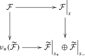
  is a pullback diagram, where all morphisms are the canonical ones and skyscraper sheaves supported at s are identified with their stalks.

Consider the comma category ${\overline{{{\,\mathrm{\mathsf {Tri}}\,}}}}(E)$ associated with a pair of functors

where $\mathbb {F}({\mathcal {G}}):= {\mathcal {G}}\Big |_{s_+} \oplus {\mathcal {G}}\Big |_{s_-}$ for any ${\mathcal {G}}\in {{\,\mathrm{\mathsf {VB}}\,}}(\mathbb {P}^1)$ and $\mathbb {G}= (\mathbb {C}\times \mathbb {C})\otimes _{\mathbb {C}} \,-\,$. By definition, any object of ${\overline{{{\,\mathrm{\mathsf {Tri}}\,}}}}(E)$ is a triple $\bigl ({\mathcal {G}}, V, \theta \bigr )$, where ${\mathcal {G}}$ is a locally free coherent sheaf on $\mathbb {P}^1$, V is a finite dimensional vector space over $\mathbb {C}$ and $\mathbb {G}(V) {\mathop {\longrightarrow }\limits ^{\theta }}\mathbb {F}({\mathcal {G}})$ is given by a pair of linear maps $V {\mathop {\longrightarrow }\limits ^{\theta _\pm }}{\mathcal {G}}\Big |_{s_\pm }$. The definition of morphisms in ${\overline{{{\,\mathrm{\mathsf {Tri}}\,}}}}(E)$ is straightforward.

The following result is a special case of [9, Theorem 16]; see also [11, Theorem 3.2].

Theorem 6.1

The functor ${{\,\mathrm{\mathsf {TF}}\,}}(E) {\mathop {\longrightarrow }\limits ^{\mathbb {E}}}{\overline{{{\,\mathrm{\mathsf {Tri}}\,}}}}(E),\; {\mathcal {F}}\mapsto \bigl ({\widetilde{{\mathcal {F}}}}, {\mathcal {F}}\big |_{s}, \theta _{{\mathcal {F}}}\bigr )$ is fully faithful. The essential image ${{\,\mathrm{\mathsf {Tri}}\,}}(E)$ of ${{\,\mathrm{\mathsf {TF}}\,}}(E)$ consists of those triples $\bigl ({\mathcal {G}}, V, \theta \bigr )$, for which both linear maps $\theta _\pm$ are surjective and the linear map $\tilde{\theta }= \left( \begin{array}{c} \theta _+ \\ \theta _- \end{array}\right) : V \longrightarrow {\mathcal {G}}\Big |_{s_+} \oplus {\mathcal {G}}\Big |_{s_-}$ is injective, whereas the essential image of the category ${{\,\mathrm{\mathsf {VB}}\,}}(E)$ consists of those triples $\bigl ({\mathcal {G}}, V, \theta \bigr )$, for which $\theta$ is an isomorphism. In other words, the functor ${{\,\mathrm{\mathsf {TF}}\,}}(E) {\mathop {\longrightarrow }\limits ^{\mathbb {E}}}{{\,\mathrm{\mathsf {Tri}}\,}}(E)$ is an equivalence of categories. Conversely, given an object ${\mathcal {T}}= \bigl ({\mathcal {G}}, V, \theta \bigr )$ of ${{\,\mathrm{\mathsf {Tri}}\,}}(E)$, consider the torsion free sheaf ${\mathcal {F}}$ on E defined as a pullback

(77)

in the category ${{\,\mathrm{\mathsf {Coh}}\,}}(E)$. Then we have: $\mathbb {E}({\mathcal {F}}) \cong {\mathcal {T}}$.

Remark 6.2

Let $({\mathcal {B}}, {{\,\mathrm{{\mathfrak {a}}}\,}}, \theta )$ be an object of ${{\,\mathrm{\mathsf {Tri}}\,}}(E)$, for which ${\mathcal {B}}$ is a sheaf of Lie algebras on $\mathbb {P}^1$, ${{\,\mathrm{{\mathfrak {a}}}\,}}$ is a Lie algebra and $\theta$ is a morphism of Lie algebras. Then the torsion free coherent sheaf ${\mathcal {A}}$ defined by the pullback diagram (77) corresponding to $({\mathcal {B}}, {{\,\mathrm{{\mathfrak {a}}}\,}}, \theta )$ is a sheaf of Lie algebras on E. It follows from (77) that the following sequences of vector spaces is exact:

$$\begin{aligned} 0 \rightarrow \Gamma (E, {\mathcal {A}}) \rightarrow \Gamma (\mathbb {P}^1, {\mathcal {B}}) \oplus {{\,\mathrm{{\mathfrak {a}}}\,}}\xrightarrow {\left( {\begin{matrix} {{\,\mathrm{\mathsf {ev}}\,}}_+ &{} \theta _+ \\ {{\,\mathrm{\mathsf {ev}}\,}}_- &{} \theta _-\end{matrix}}\right) } {\mathcal {B}}\Big |_{s_+} \oplus {\mathcal {B}}\Big |_{s_-} \rightarrow H^1(E, {\mathcal {A}}) \rightarrow H^1(\mathbb {P}^1, {\mathcal {B}}) \rightarrow 0, \end{aligned}$$

(78)

where $\Gamma (\mathbb {P}^1, {\mathcal {B}}) {\mathop {\longrightarrow }\limits ^{{{\,\mathrm{\mathsf {ev}}\,}}_\pm }}{\mathcal {B}}\Big |_{s_\pm }$ denotes the canonical evaluation map at the point $s_\pm$. $\lozenge$

6.2 Geometrization of twists of the standard Lie bialgebra structure on twisted loop algebras

Now we return to the setting of Section 3. Let ${{\,\mathrm{{\mathfrak {D}}}\,}}= {{\,\mathrm{{\mathfrak {C}}}\,}}\dotplus {{\,\mathrm{{\mathfrak {W}}}\,}}$ be a Manin triple as in Theorem 4.1. Let ${{\,\mathrm{{\mathfrak {V}}}\,}}_\pm \subset {{\,\mathrm{{\mathfrak {L}}}\,}}$ be Lie subalgebras from Lemma 4.4. Recall that ${{\,\mathrm{{\mathfrak {V}}}\,}}_\pm$ is a free module of rank q over $L_\pm = \mathbb {C}\bigl [t_{\pm }\bigr ] \subset R = \mathbb {C}\bigl [t, t^{-1}\bigr ]$, where $t_\pm = t^{\pm 1}$. In what follows, we shall view the projective line $\mathbb {P}^1$ as the pullback of the pair of morphisms

$$\begin{aligned} {{\,\mathrm{\mathsf {Spec}}\,}}(L_+) \longrightarrow {{\,\mathrm{\mathsf {Spec}}\,}}(R) \longleftarrow {{\,\mathrm{\mathsf {Spec}}\,}}(L_-), \end{aligned}$$

identifying ${{\,\mathrm{\mathsf {Spec}}\,}}(L_\pm )$ with open subsets $U_\pm \subset \mathbb {P}^1$ and ${{\,\mathrm{\mathsf {Spec}}\,}}(R)$ with $U := U_+ \cap U_-$. Let $s_\pm \in U_\pm$ be the point corresponding to the maximal ideal $(t_{\pm }) \subset L_\pm$, then $t_\pm$ is a local parameter at $s_\pm$.

Proposition 6.3

There exists a unique coherent sheaf of Lie algebras ${\mathcal {B}}$ on $\mathbb {P}^1$ such that $\Gamma (V, {\mathcal {B}}) \subset \mathbb {C}(t) \otimes _R {{\,\mathrm{{\mathfrak {L}}}\,}}$ for any open subset $V \subseteq \mathbb {P}^1$ and such that the following diagram of Lie algebras

(79)

is commutative. We have:

$$\begin{aligned} \Gamma (\mathbb {P}^1, {\mathcal {B}}) = {{\,\mathrm{{\mathfrak {V}}}\,}}_+ \cap {{\,\mathrm{{\mathfrak {V}}}\,}}_- \quad \mathrm{and} \quad H^1(\mathbb {P}^1, {\mathcal {B}}) = 0. \end{aligned}$$

(80)

The completion of the stalk of ${\mathcal {B}}$ at $s_{\pm }$ is naturally isomorphic to ${\widehat{{{\,\mathrm{{\mathfrak {W}}}\,}}}}_\pm$ as a Lie algebra over ${\widehat{L}}_\pm = \mathbb {C}\llbracket t_\pm \rrbracket$, where ${{\,\mathrm{{\mathfrak {W}}}\,}}_\pm$ is the Lie algebra from Lemma 4.4. In particular, we can identify the fiber ${\mathcal {B}}\Big |_{s_\pm }$ with the Lie algebra ${{\,\mathrm{{\mathfrak {w}}}\,}}_\pm := {\widehat{{{\,\mathrm{{\mathfrak {W}}}\,}}}}_\pm /t_\pm {\widehat{{{\,\mathrm{{\mathfrak {W}}}\,}}}}_\pm$.

Proof

Existence and uniqueness of ${\mathcal {B}}$ characterized by (79) is clear. We have the Mayer–Vietoris exact sequence

$$\begin{aligned} 0 \longrightarrow \Gamma (\mathbb {P}^1, {\mathcal {B}}) \longrightarrow \Gamma (U_+, {\mathcal {B}}) \oplus \Gamma (U_-, {\mathcal {B}}) \longrightarrow \Gamma (U, {\mathcal {B}}) \longrightarrow H^1(\mathbb {P}^1, {\mathcal {B}}) \longrightarrow 0. \end{aligned}$$

According to Lemma 4.4, we have: ${{\,\mathrm{{\mathfrak {L}}}\,}}= {{\,\mathrm{{\mathfrak {V}}}\,}}_+ + {{\,\mathrm{{\mathfrak {V}}}\,}}_-$. If follows from (79) that the formulae (80) are true. The remaining statements are obvious. $\square$

Next, we can define E via the pushout diagram (76). It follows that E is a nodal Weierstraß curve. Let ${\widehat{O}}_\pm$ be the completion of the stalk of ${\mathcal {O}}_{\mathbb {P}^1}$ at $s_\pm$, ${\widehat{O}}$ be the completion of the stalk of ${\mathcal {O}}_{E}$ at s and ${\widehat{Q}}$ be the total ring of quotients of ${\widehat{O}}$. Then we have: ${\widehat{O}}_\pm \cong \mathbb {C}\llbracket t_\pm \rrbracket$, ${\widehat{O}} \cong \mathbb {C}\llbracket t_+, t_-\rrbracket /(t_+ t_-)$ and ${\widehat{Q}} = \mathbb {C}(\!(t_+ )\!)\times \mathbb {C}(\!(t_- )\!)$. According to Lemma 4.3, the completed Lie algebra ${{\widehat{{{\,\mathrm{{\mathfrak {W}}}\,}}}}}$ is an ${\widehat{O}}$–module. We put:

$$\begin{aligned} {{\,\mathrm{{\mathfrak {w}}}\,}}:= {\widehat{{{\,\mathrm{{\mathfrak {W}}}\,}}}}/(t_+, t_-){\widehat{{{\,\mathrm{{\mathfrak {W}}}\,}}}} \subset {\widehat{{{\,\mathrm{{\mathfrak {W}}}\,}}}}_+/t_+ {\widehat{{{\,\mathrm{{\mathfrak {W}}}\,}}}}_+ \times {\widehat{{{\,\mathrm{{\mathfrak {W}}}\,}}}}_+/t_+ {\widehat{{{\,\mathrm{{\mathfrak {W}}}\,}}}}_- = {{\,\mathrm{{\mathfrak {w}}}\,}}_+ \times {{\,\mathrm{{\mathfrak {w}}}\,}}_-. \end{aligned}$$

Again, according to Lemma 4.3, the morphism of Lie algebras ${{\,\mathrm{{\mathfrak {w}}}\,}}{\mathop {\longrightarrow }\limits ^{\theta _\pm }}{{\,\mathrm{{\mathfrak {w}}}\,}}_\pm$ defined as the composition ${{\,\mathrm{{\mathfrak {w}}}\,}}\hookrightarrow {{\,\mathrm{{\mathfrak {w}}}\,}}_+ \times {{\,\mathrm{{\mathfrak {w}}}\,}}_- \twoheadrightarrow {{\,\mathrm{{\mathfrak {w}}}\,}}_\pm$ is surjective. It follows that $({{\,\mathrm{{\mathfrak {B}}}\,}}, {{\,\mathrm{{\mathfrak {w}}}\,}}, \theta )$ is an object of the category ${{\,\mathrm{\mathsf {Tri}}\,}}(E)$ from Theorem 6.1.

Proposition 6.4

Let ${\mathcal {A}}$ be the sheaf of Lie algebras on E, corresponding to the triple $({{\,\mathrm{{\mathfrak {B}}}\,}}, {{\,\mathrm{{\mathfrak {w}}}\,}}, \theta )$. Then $(E, {\mathcal {A}})$ is a geometric CYBE datum.

Proof

We keep the notation of Sect. 5.3. First observe that the canonical map ${{\,\mathrm{{\mathfrak {A}}}\,}}= \Gamma (U, {\mathcal {A}}) \rightarrow \Gamma \bigl (U, \nu _*({\mathcal {B}})\bigr ) = {{\,\mathrm{{\mathfrak {L}}}\,}}$ is an isomorphism of Lie algebras. This implies that ${\mathcal {A}}$ is ${{\,\mathrm{{\mathfrak {g}}}\,}}$–weakly locally free; see Proposition 3.4. Next, by Lemma 4.4, the linear map

$$\begin{aligned} \bigl ({{\,\mathrm{{\mathfrak {V}}}\,}}_+ \cap {{\,\mathrm{{\mathfrak {V}}}\,}}_-\bigr ) \oplus {{\,\mathrm{{\mathfrak {w}}}\,}}= \Gamma (\mathbb {P}^1, {\mathcal {B}}) \oplus {{\,\mathrm{{\mathfrak {w}}}\,}}\xrightarrow {\left( {\begin{matrix} {{\,\mathrm{\mathsf {ev}}\,}}_+ &{} \theta _+ \\ {{\,\mathrm{\mathsf {ev}}\,}}_- &{} \theta _-\end{matrix}}\right) } {\mathcal {B}}\Big |_{s_+} \oplus {\mathcal {B}}\Big |_{s_-} \cong {{\,\mathrm{{\mathfrak {w}}}\,}}_+ \oplus {{\,\mathrm{{\mathfrak {w}}}\,}}_- \end{aligned}$$

is an isomorphism. Since $H^1(\mathbb {P}^1, {\mathcal {B}}) = 0$, the exact sequence (78) implies that $H^0(E, {\mathcal {A}}) = 0 = H^1(E, {\mathcal {A}})$. Moreover, it follows from the construction of ${\mathcal {A}}$ that the canonical morphism of Lie algebras ${{\widehat{{{\,\mathrm{{\mathfrak {A}}}\,}}}}} = {\widehat{{\mathcal {A}}}}_s {\mathop {\longrightarrow }\limits ^{\nu ^*}}{\widehat{{\mathcal {B}}}}_{s_+} \times {\widehat{{\mathcal {B}}}}_{s_-} \cong {\widehat{{{\,\mathrm{{\mathfrak {W}}}\,}}}}_+ \times {\widehat{{{\,\mathrm{{\mathfrak {W}}}\,}}}}_-$ is injective and its image is the Lie algebra ${{\widehat{{{\,\mathrm{{\mathfrak {W}}}\,}}}}}$. Hence, ${\widetilde{{{\,\mathrm{{\mathfrak {A}}}\,}}}} = {\widehat{Q}} \otimes _{{\widehat{O}}} {{\widehat{{{\,\mathrm{{\mathfrak {A}}}\,}}}}}$ can be identified with the Lie algebra ${\widehat{{{\,\mathrm{{\mathfrak {D}}}\,}}}}$.

It follows from the construction of E that the differential form $\omega = \dfrac{dt}{t}$ is a generator of $\Gamma (E, \Omega _E)$. The following observation is crucial: under the isomorphism $\widetilde{{{\,\mathrm{{\mathfrak {A}}}\,}}} \rightarrow {{\widehat{{{\,\mathrm{{\mathfrak {D}}}\,}}}}}$ the bilinear form ${\widetilde{{{\,\mathrm{{\mathfrak {A}}}\,}}}} \times {\widetilde{{{\,\mathrm{{\mathfrak {A}}}\,}}}} {\mathop {\longrightarrow }\limits ^{{\widetilde{F}}^\omega _s}}\mathbb {C}$ given by (63) gets identified (up to an appropriate rescaling) with the bilinear form ${\widehat{{{\,\mathrm{{\mathfrak {D}}}\,}}}} \times {\widehat{{{\,\mathrm{{\mathfrak {D}}}\,}}}} {\mathop {\longrightarrow }\limits ^{{\widehat{F}}}}\mathbb {C}$, given by (28)! Summing up, ${\widetilde{{{\,\mathrm{{\mathfrak {A}}}\,}}}} = {{\widehat{{{\,\mathrm{{\mathfrak {A}}}\,}}}}} \dotplus {{\,\mathrm{{\mathfrak {A}}}\,}}$ is a Manin triple, isomorphic to the Manin triple ${\widehat{{{\,\mathrm{{\mathfrak {D}}}\,}}}} = {\widehat{{{\,\mathrm{{\mathfrak {W}}}\,}}}} \dotplus {{\,\mathrm{{\mathfrak {C}}}\,}}$. In particular, ${{\widehat{{{\,\mathrm{{\mathfrak {A}}}\,}}}}}$ is an isotropic Lie subalgebra of ${\widetilde{{{\,\mathrm{{\mathfrak {A}}}\,}}}}$.

All together, we have proven that ${\mathcal {A}}$ is an acyclic, ${{\,\mathrm{{\mathfrak {g}}}\,}}$–weakly locally free isotropic coherent sheaf of Lie algebras on E, as asserted. $\square$

Let $(E, {\mathcal {A}})$ be a geometric datum as in Proposition 6.4 above and $\rho \in \Gamma \bigl (U \times U \setminus \Sigma , {\mathcal {A}}\boxtimes {\mathcal {A}}\bigr )$ the corresponding geometric r–matrix. Recall that the construction of ${\mathcal {A}}$ also provides an isomorphism of Lie algebras ${{\,\mathrm{{\mathfrak {A}}}\,}}{\mathop {\longrightarrow }\limits ^{\cong }}{{\,\mathrm{{\mathfrak {L}}}\,}}$. Let ${\widetilde{U}} = {{\,\mathrm{\mathsf {Spec}}\,}}({\overline{R}}) {\mathop {\longrightarrow }\limits ^{\pi }}U = {{\,\mathrm{\mathsf {Spec}}\,}}(R)$ be the étale covering corresponding to the algebra extension $R \subseteq {\overline{R}}$. By Proposition 3.4, we have an isomorphism of Lie algebras $\Gamma \bigl ({\widetilde{U}}, \pi ^*({\mathcal {A}})\bigr ) \cong {\overline{R}} \otimes _{R} {{\,\mathrm{{\mathfrak {L}}}\,}}\cong {\overline{{{\,\mathrm{{\mathfrak {L}}}\,}}}}$. The pullback

$$\begin{aligned} \tilde{\rho }:= (\pi \times \pi )^*(\rho ) \in \Gamma \bigl ({\widetilde{U}} \times {\widetilde{U}} \setminus \widetilde{\Sigma }, \pi ^*({\mathcal {A}}) \boxtimes \pi ^*({\mathcal {A}})\bigr ) \end{aligned}$$

(81)

satisfies the equalities (54) and (55), where ${\widetilde{\Sigma }} = (\pi \times \pi )^{-1}(\Sigma )$. Trivializing $\pi ^*({\mathcal {A}})$ as above, we get from $\tilde{\rho }$ a genuine skew-symmetric non-degenerate solution of the classical Yang–Baxter Eq. (36). Our next goal is to compute this solution explicitly.

6.3 Geometric r–matrix corresponding to twists of the standard Lie bialgebra structure of a twisted loop algebra

Recall our notation: ${{\,\mathrm{{\mathfrak {g}}}\,}}$ is a finite dimensional complex simple Lie algebra of dimension q, $\sigma \in {{\,\mathrm{\mathsf {Aut}}\,}}_{\mathbb {C}}({{\,\mathrm{{\mathfrak {g}}}\,}})$ is an automorphism of order m, ${{\,\mathrm{{\mathfrak {g}}}\,}}= \oplus _{k = 0}^{m-1} {{\,\mathrm{{\mathfrak {g}}}\,}}_{k}$ the corresponding decomposition of ${{\,\mathrm{{\mathfrak {g}}}\,}}$ into a direct sum of eigenspaces of $\sigma$, $\gamma = \sum \limits _{k = 0}^{m-1} \gamma _{k}$ the decomposition of the Casimir element $\gamma \in {{\,\mathrm{{\mathfrak {g}}}\,}}\otimes {{\,\mathrm{{\mathfrak {g}}}\,}}$ with components $\gamma _{k} \in {{\,\mathrm{{\mathfrak {g}}}\,}}_{k} \otimes {{\,\mathrm{{\mathfrak {g}}}\,}}_{-k}$. Let ${{\,\mathrm{{\mathfrak {g}}}\,}}_{0} = {{\,\mathrm{{\mathfrak {g}}}\,}}_{0}^+ \oplus {{\,\mathrm{{\mathfrak {h}}}\,}}\oplus {{\,\mathrm{{\mathfrak {g}}}\,}}_{0}^-$ be a triangular decomposition as in Remark 3.6. We denote by $\gamma _{0}^{0}$ and $\gamma _{0}^{\pm }$ the projections of $\gamma _0$ on ${{\,\mathrm{{\mathfrak {h}}}\,}}\otimes {{\,\mathrm{{\mathfrak {h}}}\,}}$ and ${{\,\mathrm{{\mathfrak {g}}}\,}}_{0}^\pm \otimes {{\,\mathrm{{\mathfrak {g}}}\,}}_{0}^\mp$, respectively.

Proposition 6.5

Let ${{\,\mathrm{{\mathfrak {D}}}\,}}= {{\,\mathrm{{\mathfrak {C}}}\,}}\dotplus {{\,\mathrm{{\mathfrak {W}}}\,}}^\circ$ be the Manin triple (30), corresponding to the standard Lie bialgebra cobracket ${{\,\mathrm{{\mathfrak {L}}}\,}}{\mathop {\longrightarrow }\limits ^{\delta _\circ }}\wedge ^2({{\,\mathrm{{\mathfrak {L}}}\,}})$ and $(E, {\mathcal {A}}_\circ )$ be the corresponding geometric CYBE datum defined in Proposition 6.4. Then the trivialization of the corresponding geometric r-matrix (81) gives the following solution of (36):

$$\begin{aligned} r_\circ (x, y) = \left( \frac{\gamma _{0}^{0}}{2} + \gamma _{0}^-\right) + \frac{y^m}{x^m - y^m} \sum \limits _{k = 0}^{m-1} \left( \frac{x}{y}\right) ^k \gamma _k. \end{aligned}$$

(82)

Proof

Let $q_k = \dim _{\mathbb {C}}\bigl ({{\,\mathrm{{\mathfrak {g}}}\,}}_k\bigr )$ for $k \in \mathbb {Z}$. By Lemma 3.2, we can choose a basis $\bigl (g_k^{(1)}, \dots , g_k^{(q_k)}\bigr )$ of ${{\,\mathrm{{\mathfrak {g}}}\,}}_k$ such that $\kappa \Bigl (g_k^{(i)}, g_{-k}^{(j)}\Bigr ) = \delta _{ij}$ for all $1 \le i, j \le q_k$. For $k = 0$ we make an additional choice: let $(h_1, \dots , h_r)$ be a basis of ${{\,\mathrm{{\mathfrak {h}}}\,}}$ and $(e_1^\pm , \dots , e_{p}^\pm )$ a basis of ${{\,\mathrm{{\mathfrak {g}}}\,}}_0^\pm$ such that

$$\begin{aligned} \kappa (h_\imath , h_\jmath ) = \delta _{\imath \jmath } \; \text{ for } \text{ all }\; 1 \le \imath , \jmath \le r \; \text{ and }\; \kappa (e_\imath ^+, e_\jmath ^-) = \delta _{\imath \jmath } \; \text{ for } \text{ all }\; 1 \le \imath , \jmath \le p. \end{aligned}$$

Then we have the following basis of ${{\,\mathrm{{\mathfrak {L}}}\,}}= \bigoplus \limits _{k \in \mathbb {Z}} {{\,\mathrm{{\mathfrak {g}}}\,}}_k z^k$ viewed as a module over $R = \mathbb {C}\bigl [t, t^{-1}\bigr ]$:

$$\begin{aligned} \bigl (e_1^+, \dots , e_p^+, h_1, \dots , h_r, e_1^-, \dots , e_p^-, g_{1}^{(1)} z, \dots , g_{1}^{(q_1)} z, \dots , g_{m-1}^{(1)} z^{m-1}, \dots , g_{m-1}^{(q_{m-1})} z^{m-1}\bigr ) \end{aligned}$$

(83)

where $t = z^m$. As usual, let ${{\,\mathrm{{\mathfrak {L}}}\,}}\times {{\,\mathrm{{\mathfrak {L}}}\,}}{\mathop {\longrightarrow }\limits ^{K}}R$ be the Killing form. For any $\lambda \in \mathbb {C}^*$, let $\bigl (R/(t-\lambda )\bigr ) \otimes _{R} {{\,\mathrm{{\mathfrak {L}}}\,}}{\mathop {\longrightarrow }\limits ^{\varepsilon _\lambda }}{{\,\mathrm{{\mathfrak {g}}}\,}}$ be the Lie algebra isomorphism from Proposition 3.4 and $R {\mathop {\longrightarrow }\limits ^{{{\,\mathrm{\mathsf {ev}}\,}}_\lambda }}\mathbb {C}$ be the evaluation map. Then the diagram

is commutative and

$$\begin{aligned} \bigl (e_1^-, \dots , e_p^-, h_1, \dots , h_r, e_1^+, \dots , e_p^+, g_{-1}^{(1)} z^{-1}, \dots , g_{-1}^{(q_1)} z^{-1}, \dots , g_{1-m}^{(1)} z^{1-m}, \dots , g_{1-m}^{(q_{m-1})} z^{1-m}\bigr ) \end{aligned}$$

is the basis of ${{\,\mathrm{{\mathfrak {L}}}\,}}$ over R which is dual to (83) with respect to the Killing form K. Hence,

$$\begin{aligned} \chi = \left( \sum \limits _{\imath = 1}^p \bigl (e_\imath ^+ \otimes e_\imath ^- + e_\imath ^- \otimes e_\imath ^+ \bigr ) + \sum \limits _{l = 1}^r h_l \otimes h_l\right) + \left( \sum \limits _{k = 1}^{m-1} \sum \limits _{j = 1}^{q_k} g_k^{(j)} z^k \otimes g_{-k}^{(j)} z^{-k}\right) \in {{\,\mathrm{{\mathfrak {L}}}\,}}\otimes _R {{\,\mathrm{{\mathfrak {L}}}\,}}\end{aligned}$$

is the canonical Casimir element of ${{\,\mathrm{{\mathfrak {L}}}\,}}$ (viewed as a Lie algebra over R).

We identify $\rho$ with $\tilde{\rho } \in \Gamma \bigl ({\widetilde{U}} \times {\widetilde{U}} \setminus \widetilde{\Sigma }, \pi ^*({\mathcal {A}}) \boxtimes \pi ^*({\mathcal {A}})\bigr )$. To proceed with computations, we make the following choices: let (u, v) be coordinates on $\mathbb {C}^*\times \mathbb {C}^*\cong U \times U$ and (x, y) be coordinates on the étale covering $\mathbb {C}^*\times \mathbb {C}^*\cong {\widetilde{U}} \times {\widetilde{U}}$. We have: $u = x^m$ and $v = y^m$. Consider the following expression:

$$\begin{aligned} \widetilde{\chi } := \sum \limits _{k = 0}^{m-1} \gamma _k \left( \dfrac{x}{y}\right) ^k \in {{\,\mathrm{{\mathfrak {L}}}\,}}\otimes _{\mathbb {C}} {{\,\mathrm{{\mathfrak {L}}}\,}}\subseteq ({{\,\mathrm{{\mathfrak {g}}}\,}}\otimes {{\,\mathrm{{\mathfrak {g}}}\,}})\bigl [x, x^{-1}, y, y^{-1}\bigr ]. \end{aligned}$$

It is easy to see that $\widetilde{\chi }$ is mapped to $\chi$ under the canonical linear map ${{\,\mathrm{{\mathfrak {L}}}\,}}\otimes _{\mathbb {C}} {{\,\mathrm{{\mathfrak {L}}}\,}}\twoheadrightarrow {{\,\mathrm{{\mathfrak {L}}}\,}}\otimes _{R} {{\,\mathrm{{\mathfrak {L}}}\,}}$.

Recall that the geometric r-matrix $\rho$ corresponding to $(E, {\mathcal {A}})$ is given by the formula (74). For any $(k, i) \in \Upsilon$ we have $w_{(k, i)} \in {\widehat{{{\,\mathrm{{\mathfrak {D}}}\,}}}}$, given by the formula (69) with respect to the R-basis of ${{\,\mathrm{{\mathfrak {L}}}\,}}$ fixed above. Then there exist uniquely determined $b_{(k, i)} \in {\widehat{{{\,\mathrm{{\mathfrak {W}}}\,}}}}^\circ$ and $h_{(k, i)} \in {{\,\mathrm{{\mathfrak {L}}}\,}}\cong {{\,\mathrm{{\mathfrak {C}}}\,}}$ such that $b_{(k,\, i)} = w_{(k,\, i)} + h_{(k,\, i)}$. It is not hard to see that $h_{(k, i)} = 0$ for all $k \ne 0$. For $k = 0$, we have the following decompositions:

$$\begin{aligned} {\widehat{{{\,\mathrm{{\mathfrak {W}}}\,}}}}^\circ \ni \left\{ \begin{array}{ccl} (0, e_\imath ^-) &{} = &{} (-e_\imath ^-, 0) + (e_\imath ^-, e_\imath ^-) \\ (-e_\imath ^+, 0) &{} = &{} (-e_\imath ^+, 0) + (0, 0) \\ \left( -\frac{1}{2} h_l, \frac{1}{2} h_l\right) &{} = &{} (-h_l, 0) + \left( \frac{1}{2} h_l, \frac{1}{2} h_l\right) . \end{array} \right. \end{aligned}$$

All together, taking into account the formulae (69), (70) and (71), we obtain from (74) the following explicit expression:

$$\begin{aligned} r_\circ (x, y) = \frac{y^m}{x^m - y^m} \sum \limits _{k = 0}^{m-1} \left( \frac{x}{y}\right) ^k \gamma _k + \left( \sum \limits _{\imath = 1}^p e_\imath ^- \otimes e_\imath ^+ + \sum \limits _{l = 1}^r \frac{1}{2} h_l \otimes h_l\right) , \end{aligned}$$

which coincides with the formula (82), as asserted. $\square$

We get the following corollary, which seems to be well-known to the experts (another, more direct proof, can be found in [1]).

Corollary 6.6

We have the following formula for the standard Lie bialgebra cobracket:

$$\begin{aligned} {{\,\mathrm{{\mathfrak {L}}}\,}}{\mathop {\longrightarrow }\limits ^{\delta _\circ }}{{\,\mathrm{{\mathfrak {L}}}\,}}\wedge {{\,\mathrm{{\mathfrak {L}}}\,}}, \quad f(z) \mapsto \bigl [f(x) \otimes 1 + 1 \otimes f(y), r_\circ (x,y)\bigr ], \end{aligned}$$

where $r_\circ (x, y)$ is the standard r-matrix given by (82).

Remark 6.7

Let ${{\,\mathrm{{\mathfrak {g}}}\,}}= {{\,\mathrm{{\mathfrak {n}}}\,}}^{+} \dotplus {\tilde{{{\,\mathrm{{\mathfrak {h}}}\,}}}} \dotplus {{\,\mathrm{{\mathfrak {n}}}\,}}^{-}$ be a fixed triangular decomposition of the finite dimensional simple complex Lie algebra ${{\,\mathrm{{\mathfrak {g}}}\,}}$ corresponding to a Dynkin diagram $\Gamma$. Then any $\phi \in {{\,\mathrm{\mathsf {Aut}}\,}}(\Gamma )$ defines an automorphism ${\tilde{\phi }} \in {{\,\mathrm{\mathsf {Aut}}\,}}_{\mathbb {C}}({{\,\mathrm{{\mathfrak {g}}}\,}})$. Let $\sigma \in {{\,\mathrm{\mathsf {Aut}}\,}}_{\mathbb {C}}({{\,\mathrm{{\mathfrak {g}}}\,}})$ be a Coxeter automorphism corresponding to $\phi$ and m be the order of $\sigma$; see [6, Section 6] for an explicit description of $\sigma$. Then we have: ${{\,\mathrm{{\mathfrak {L}}}\,}}:= {{\,\mathrm{{\mathfrak {L}}}\,}}({{\,\mathrm{{\mathfrak {g}}}\,}}, \sigma ) \cong {{\,\mathrm{{\mathfrak {L}}}\,}}({{\,\mathrm{{\mathfrak {g}}}\,}}, {\tilde{\phi }})$; see [31, Proposition 8.1]. An advantage to use the Coxeter automorphism $\sigma$ to define twisted loop algebra is due to the fact that the fixed point Lie algebra $\left\{ a \in {{\,\mathrm{{\mathfrak {g}}}\,}}\, \big | \, \sigma (a) = a \right\}$ is abelian. In particular, the standard r-matrix (82) takes the following shape:

$$\begin{aligned} r_\circ (x, y) = \frac{\gamma _{0}}{2} + \frac{y^m}{x^m - y^m} \sum \limits _{k = 0}^{m-1} \left( \frac{x}{y}\right) ^k \gamma _k = \frac{\gamma _{0}}{2} + \frac{1}{\exp (w) -1} \sum \limits _{k = 0}^{m-1} \exp \left( \frac{k w}{m}\right) \gamma _j, \end{aligned}$$

(84)

where $\exp \left( \dfrac{w}{m}\right) = \dfrac{x}{y}$. For $\phi = \mathsf {id}$, this solution was discovered for the first time by Kulish (see [38, formula (38)]) and generalized by Belavin and Drinfeld (see [6, Proposition 6.1]) for an arbitrary $\phi$.

Remark 6.8

Let ${{\,\mathrm{{\mathfrak {g}}}\,}}= {{\,\mathrm{{\mathfrak {n}}}\,}}^{+} \dotplus {\tilde{{{\,\mathrm{{\mathfrak {h}}}\,}}}} \dotplus {{\,\mathrm{{\mathfrak {n}}}\,}}^{-}$ be again a fixed triangular decomposition of ${{\,\mathrm{{\mathfrak {g}}}\,}}$, $\Phi _+$ be the set of positive roots of $({{\,\mathrm{{\mathfrak {g}}}\,}}, {{\,\mathrm{{\mathfrak {h}}}\,}})$ and $\sigma = \mathsf {id}$. Then ${{\,\mathrm{{\mathfrak {L}}}\,}}= {{\,\mathrm{{\mathfrak {L}}}\,}}({{\,\mathrm{{\mathfrak {g}}}\,}}, \sigma ) = {{\,\mathrm{{\mathfrak {g}}}\,}}\bigl [z, z^{-1}\bigr ]$ and the standard r-matrix (82) takes the following form:

$$\begin{aligned} r_{\circ }(x, y) = \dfrac{1}{2}\Bigl (\dfrac{x+y}{x-y} \gamma + \sum \limits _{\alpha \in \Phi _+} e_{-\alpha } \wedge e_{\alpha }\Bigr ), \end{aligned}$$

(85)

which can be for instance found in [36]. It can be shown that the solution (85) is equivalent (in the sense of (38) and (39)) to the solution (84) (for the identity automorphism of the Dynkin diagram of ${{\,\mathrm{{\mathfrak {g}}}\,}}$); see for instance [1] for details. $\lozenge$

Theorem 6.9

For any skew-symmetric tensor $\texttt {t}\in \wedge ^2{{\,\mathrm{{\mathfrak {L}}}\,}}\subset ({{\,\mathrm{{\mathfrak {g}}}\,}}\otimes {{\,\mathrm{{\mathfrak {g}}}\,}})\bigl [x, x^{-1}, y, y^{-1}\bigr ]$ we put:

$$\begin{aligned} \delta _\texttt {t}= \delta _\circ + \partial _{\texttt {t}} \quad \text{ and } \quad r_{\texttt {t}}(x, y) = r_\circ (x, y) + \texttt {t}(x, y). \end{aligned}$$

(86)

Then ${{\,\mathrm{{\mathfrak {L}}}\,}}{\mathop {\longrightarrow }\limits ^{\delta _\texttt {t}}}{{\,\mathrm{{\mathfrak {L}}}\,}}\wedge {{\,\mathrm{{\mathfrak {L}}}\,}}$ is a Lie bialgebra cobracket if and only if $r_\texttt {t}(x, y)$ is a solution of the classical Yang–Baxter Eq. (36). In this case, let ${{\,\mathrm{{\mathfrak {D}}}\,}}= {{\,\mathrm{{\mathfrak {W}}}\,}}_\texttt {t}\dotplus {{\,\mathrm{{\mathfrak {C}}}\,}}$ be the corresponding Manin triple (see Theorem 4.1) and $(E, {\mathcal {A}}_\texttt {t})$ be the corresponding geometric CYBE datum (see Proposition 6.4). Then the geometric r-matrix $\rho _\texttt {t}$ of $(E, {\mathcal {A}}_\texttt {t})$ with respect to the trivialization, described at the end of Sect. 6.2, coincides with $r_\texttt {t}(x, y)$.

Proof

By Proposition 3.4, ${{\,\mathrm{{\mathfrak {L}}}\,}}^{\otimes 3}$ does not have any non-zero ad-invariant elements. Hence, Proposition 2.3 implies that $\delta _{\texttt {t}}$ is a Lie bialgebra cobracket if and only if $\texttt {t}$ satisfies the twist Eq. (6). On the other hand, since $r_\circ$ solves the CYBE, we can rewrite the CYBE for $r_\texttt {t}$ as

$$\begin{aligned}{}[[\texttt {t}, \texttt {t}]] + \bigl [r_\circ ^{12}, \texttt {t}^{13} + \texttt {t}^{23}\bigr ] + \bigl [r_\circ ^{13}, \texttt {t}^{23} + \texttt {t}^{21}\bigr ] + \bigl [r_\circ ^{23}, \texttt {t}^{21} + \texttt {t}^{31}\bigr ] = 0. \end{aligned}$$

We have: $\bigl [r_\circ ^{12}, \texttt {t}^{13} + \texttt {t}^{23}\bigr ] = - (\delta _\circ \otimes \mathbb {1})(\texttt {t})$. It follows that $r_\texttt {t}$ solves the CYBE if and only if ${{\,\mathrm{\mathsf {alt}}\,}}\bigl ((\delta _\circ \otimes \mathbb {1})(\texttt {t})\bigr ) = [[\texttt {t}, \texttt {t}]],$ implying the first statement.

As it was explained in the proof of Proposition 6.4, the Manin triple ${\widehat{{{\,\mathrm{{\mathfrak {D}}}\,}}}} = {\widehat{{{\,\mathrm{{\mathfrak {W}}}\,}}}}_\texttt {t}\dotplus {{\,\mathrm{{\mathfrak {C}}}\,}}$ is isomorphic to the geometric Manin triple ${\widetilde{{{\,\mathrm{{\mathfrak {A}}}\,}}}} = {{\widehat{{{\,\mathrm{{\mathfrak {A}}}\,}}}}}_{\texttt {t}} \dotplus {{\,\mathrm{{\mathfrak {A}}}\,}}$. Let ${\tilde{r}}_\texttt {t}(x, y)$ be the trivialization of the geometric r-matrix $\rho _\texttt {t}$ with respect to the trivialization ${{\,\mathrm{{\mathfrak {A}}}\,}}\cong {{\,\mathrm{{\mathfrak {L}}}\,}}$ introduced at the end of Sect. 6.2. Then we get the geometric Lie bialgebra cobracket

$$\begin{aligned} {{\,\mathrm{{\mathfrak {L}}}\,}}{\mathop {\longrightarrow }\limits ^{\delta }}{{\,\mathrm{{\mathfrak {L}}}\,}}\wedge {{\,\mathrm{{\mathfrak {L}}}\,}}, \; f(z) \mapsto \bigl [f(x) \otimes 1 + 1 \otimes f(y), {\tilde{r}}_\texttt {t}(x, y)\bigr ]. \end{aligned}$$

On the other hand, Corollary 6.6 implies that

$$\begin{aligned} \delta _\texttt {t}(f)&:= \delta _\circ (f) + \bigl [f(x) \otimes 1 + 1 \otimes f(y), \texttt {t}(x, y)\bigr ] \\&= \bigl [f(x) \otimes 1 + 1 \otimes f(y), r_\circ (x, y) + \texttt {t}(x, y)\bigr ]. \end{aligned}$$

According to Proposition 4.5 and Theorem 5.6, both Lie bialgebra cobrackets $\delta$ and $\delta _\texttt {t}$ are determined by the same Manin triple ${\widehat{{{\,\mathrm{{\mathfrak {D}}}\,}}}} = {\widehat{{{\,\mathrm{{\mathfrak {W}}}\,}}}}_\texttt {t}\dotplus {{\,\mathrm{{\mathfrak {C}}}\,}}$. It follows that $\delta = \delta _\texttt {t}$. Since ${{\,\mathrm{{\mathfrak {L}}}\,}}^{\otimes 2}$ has no non-zero ad-invariant elements (see Proposition 3.4), we conclude that ${\tilde{r}}_\texttt {t}(x, y) = r_\circ (x, y) + \texttt {t}(x, y) = r_\texttt {t}(x, y)$, as asserted. $\square$

6.4 On the Theory of trigonometric solutions of CYBE

Consider the setting of Remark 6.7. Let ${{\,\mathrm{{\mathfrak {g}}}\,}}= {{\,\mathrm{{\mathfrak {n}}}\,}}^{+} \dotplus {\tilde{{{\,\mathrm{{\mathfrak {h}}}\,}}}} \dotplus {{\,\mathrm{{\mathfrak {n}}}\,}}^{-}$ be a triangular decomposition of ${{\,\mathrm{{\mathfrak {g}}}\,}}$, $\Gamma$ be the Dynkin diagram of ${{\,\mathrm{{\mathfrak {g}}}\,}}$ and $\phi \in {{\,\mathrm{\mathsf {Aut}}\,}}(\Gamma )$. Let $\sigma \in {{\,\mathrm{\mathsf {Aut}}\,}}_{\mathbb {C}}({{\,\mathrm{{\mathfrak {g}}}\,}})$ be a Coxeter automorphism corresponding to $\phi$, m be the order of $\sigma$ and ${{\,\mathrm{{\mathfrak {L}}}\,}}:= {{\,\mathrm{{\mathfrak {L}}}\,}}({{\,\mathrm{{\mathfrak {g}}}\,}}, \sigma )$. Recall that ${{\,\mathrm{{\mathfrak {g}}}\,}}_{0} = {{\,\mathrm{{\mathfrak {h}}}\,}}$ is an abelian Lie algebra. For $1 \le k \le m-1$ and $\alpha \in {{\,\mathrm{{\mathfrak {h}}}\,}}^*$, let ${{\,\mathrm{{\mathfrak {g}}}\,}}_{k}^\alpha := \bigl \{x \in {{\,\mathrm{{\mathfrak {g}}}\,}}_{k} \, \big | \, [h, x] = \alpha (h)x \; \mathrm{for all} \; h \in {{\,\mathrm{{\mathfrak {h}}}\,}}\bigr \}.$ We put

$$\begin{aligned} \Lambda _k := \bigl \{\alpha \in {{\,\mathrm{{\mathfrak {h}}}\,}}^*\, \big | \, {{\,\mathrm{{\mathfrak {g}}}\,}}_{k}^\alpha \ne 0 \bigr \} \quad \mathrm{and} \quad \Xi := \left\{ (\alpha , k) \, \big | \, 1 \le k \le m - 1 \; \text{ and } \; \alpha \in \Lambda _k \right\} . \end{aligned}$$

Then we have a direct sum decomposition

$$\begin{aligned} {{\,\mathrm{{\mathfrak {g}}}\,}}= {{\,\mathrm{{\mathfrak {h}}}\,}}\oplus \bigoplus _{(\alpha , k) \in \Xi } {{\,\mathrm{{\mathfrak {g}}}\,}}_{k}^{\alpha }, \end{aligned}$$

(87)

and the vector space ${{\,\mathrm{{\mathfrak {g}}}\,}}_{k}^\alpha$ is one-dimensional for any $(\alpha , k) \in \Xi$.

The main advantage to define the twisted loop algebra ${{\,\mathrm{{\mathfrak {L}}}\,}}$ corresponding to $\nu \in {{\,\mathrm{\mathsf {Aut}}\,}}(\Gamma )$ using a Coxeter automorphism (even for $\phi = \mathsf {id}$) is due to the following special structure of the set $\Pi$ of positive simple roots of $({{\,\mathrm{{\mathfrak {L}}}\,}}, {{\,\mathrm{{\mathfrak {h}}}\,}})$: $\Pi = \bigl \{(\alpha , 1) \, \big | \, \alpha \in \Lambda _1\bigr \}.$ In particular, we have: $\big |\Lambda _1\big | = r + 1= \dim _{\mathbb {C}}({{\,\mathrm{{\mathfrak {h}}}\,}}) + 1$ and the elements of $\Lambda _1$ are in a bijection with the vertices of the affine Dynkin diagram ${\widehat{\Gamma }}$ such that ${{\,\mathrm{{\mathfrak {L}}}\,}}\cong {{\,\mathrm{{\mathfrak {G}}}\,}}_{{\widehat{\Gamma }}}$ via the Gabber–Kac isomorphism (20).

Recall that a Belavin–Drinfeld triple is a tuple $\bigl (\Gamma _1, \Gamma _2, \tau \bigr )$, where $\Gamma _i \subsetneqq \Lambda _1$ for $i = 1, 2$ are subsets and $\Gamma _1 {\mathop {\longrightarrow }\limits ^{\tau }}\Gamma _2$ is a bijection satisfying the following conditions:

• $\kappa \bigl (\tau (\alpha ), \tau (\beta )\bigr ) = \kappa (\alpha , \beta )$ for all $\alpha , \beta \in \Gamma _1$;

• for any $\alpha \in \Gamma _1$ there exists $l = l(\alpha ) \in \mathbb {N}$ such that $\alpha , \dots , \tau ^{l-1}(\alpha ) \in \Gamma _1$ but $\tau ^l(\alpha ) \notin \Gamma _1$.

For $i = 1, 2$, let ${{\,\mathrm{{\mathfrak {n}}}\,}}_i$ be the Lie subalgebra of ${{\,\mathrm{{\mathfrak {g}}}\,}}$ generated by the vector subspace $\oplus _{\alpha \in \Gamma _i} {{\,\mathrm{{\mathfrak {g}}}\,}}_1^{\alpha }$. Then ${{\,\mathrm{{\mathfrak {n}}}\,}}_i$ is isomorphic to the positive part of the semisimple Lie algebra defined by the Dynkin diagram $\Gamma _i$ and we have a direct sum decomposition

$$\begin{aligned} {{\,\mathrm{{\mathfrak {n}}}\,}}_i = \bigoplus _{(\alpha , k) \in \Xi _i} {{\,\mathrm{{\mathfrak {g}}}\,}}_{k}^{\alpha }. \end{aligned}$$

(88)

for an appropriate subset $\Xi _i \subset \Xi$. Fixing non-zero elements in $\left( {{\,\mathrm{{\mathfrak {g}}}\,}}_1^\alpha \right) _{\alpha \in \Lambda _1}$, one can extend the bijection $\Gamma _1 {\mathop {\longrightarrow }\limits ^{\tau }}\Gamma _2$ to an isomorphism of Lie algebras ${{\,\mathrm{{\mathfrak {n}}}\,}}_1 {\mathop {\longrightarrow }\limits ^{{\tilde{\tau }}}}{{\,\mathrm{{\mathfrak {n}}}\,}}_2$.

Let ${{\,\mathrm{{\mathfrak {g}}}\,}}{\mathop {\longrightarrow }\limits ^{\vartheta }}{{\,\mathrm{{\mathfrak {g}}}\,}}$ be a linear map defined as the composition where $\pi$ and $\imath$ are the canonical projection and embedding with respect to the direct sum decompositions (87) and (88). Then $\vartheta$ is nilpotent and $\vartheta ({{\,\mathrm{{\mathfrak {g}}}\,}}_k) \subset {{\,\mathrm{{\mathfrak {g}}}\,}}_k$ for all $1 \le k \le m-1$. Let $\psi = \dfrac{\vartheta }{\mathbb {1} - \vartheta } = \sum \limits _{l = 1}^\infty \vartheta ^l.$ It follows that $\psi ({{\,\mathrm{{\mathfrak {g}}}\,}}_k) \subset {{\,\mathrm{{\mathfrak {g}}}\,}}_k$ for all $1 \le k \le m-1$ as well.

For any Belavin–Drinfeld triple $\bigl (\Gamma _1, \Gamma _2, \tau \bigr )$, the system of linear equations

$$\begin{aligned} \bigl (\tau (\alpha ) \otimes \mathbb {1} + \mathbb {1} \otimes \alpha \bigr )\Bigl (\texttt {s}+ \frac{\gamma _{0}}{2}\Bigr ) = 0 \quad \text{ for } \text{ all } \; \alpha \in \Gamma _1 \end{aligned}$$

(89)

for $\texttt {s}\in {{\,\mathrm{{\mathfrak {h}}}\,}}\wedge {{\,\mathrm{{\mathfrak {h}}}\,}}$ is consistent; see [6, Lemma 6.8]. According to [6, Theorem 6.1], trigonometric solutions of (41) are parametrized by Belavin–Drinfeld quadruples $Q = \bigl (\bigl (\Gamma _1, \Gamma _2, \tau \bigr ), \texttt {s}\bigr )$, where $\bigl (\Gamma _1, \Gamma _2, \tau \bigr )$ is a Belavin–Drinfeld triple and $\texttt {s}\in {{\,\mathrm{{\mathfrak {h}}}\,}}\wedge {{\,\mathrm{{\mathfrak {h}}}\,}}$ satisfies (89). The solution of (41) corresponding to Q is given by the following formula:

$$\begin{aligned} \varrho _Q(w) = \varrho _\circ (w) + \texttt {s}+ \sum \limits _{j = 1}^{m-1} \left( - \exp \left( \frac{jw}{m}\right) (\psi \otimes \mathbb {1}) \gamma _j + \exp \left( -\frac{jw}{m}\right) (\mathbb {1} \otimes \psi ) \gamma _{-j}\right) , \end{aligned}$$

(90)

where $\varrho _\circ (w)$ is given by (84).

Let us rewrite the formula (90) in different terms. Choose elements $\bigl (g_{(\alpha , k)} \in {{\,\mathrm{{\mathfrak {g}}}\,}}_{k}^\alpha \bigr )_{(\alpha , k) \in \Xi }$ such that $\kappa \bigl (g_{(\alpha , k)}, g_{(\beta , l)}\bigr ) = \delta _{\alpha +\beta , 0} \delta _{k+l, 0}$. Then for any $1 \le k \le m-1$ we have: $\gamma _{\pm k} = \sum \limits _{\alpha \in \Xi _{\pm k}} g_{(\pm \alpha , \pm k)} \otimes g_{(\mp \alpha , \mp k)}.$ It follows that

$$\begin{aligned} \left\{ \begin{array}{l} (\psi \otimes \mathbb {1})(\gamma _k) \; \, = \sum \limits _{l = 1}^\infty \sum \limits _{\alpha \in \Xi _k} \vartheta ^l\bigl (g_{(\alpha , k)}) \otimes g_{(-\alpha , -k)} \\ (\mathbb {1} \otimes \psi )(\gamma _{-k}) = \sum \limits _{l = 1}^\infty \sum \limits _{\alpha \in \Xi _k} g_{(-\alpha , -k)} \otimes \vartheta ^l\bigl (g_{(\alpha , k)}). \end{array} \right. \end{aligned}$$

Consider the following expression

$$\begin{aligned} t_Q(x, y) := \texttt {s}+ \sum \limits _{l = 1}^\infty \sum \limits _{(\alpha , k) \in \Xi } \bigl (-\vartheta ^l\bigl (g_{(\alpha , k)}\bigr ) \otimes g_{(-\alpha , -k)} \left( \frac{x}{y}\right) ^k + g_{(-\alpha , -k)} \otimes \vartheta ^l\bigl (g_{(\alpha , k)}\bigr ) \left( \frac{y}{x}\right) ^k\Bigr ). \end{aligned}$$

(91)

Then we have:

$$\begin{aligned} r_Q(x, y) := r_\circ (x, y) + t_Q(x, y) = \varrho _Q(w) \end{aligned}$$

(92)

where x, y and w are related by the formula $\dfrac{x}{y} = \exp \left( \dfrac{w}{m}\right)$. In other words, $r_Q$ is the solution of the classical Yang–Baxter Eq. (36) corresponding to the Belavin–Drinfeld quadruple $Q = \bigl ((\Gamma _1, \Gamma _2, \tau ), \texttt {s}\bigr )$.

Corollary 6.10

For $az^k, bz^l \in {\overline{{{\,\mathrm{{\mathfrak {L}}}\,}}}}$ we put: $az^k \wedge b z^l := a x^k \otimes b y^l - b x^l \otimes a y^k \in {\overline{{{\,\mathrm{{\mathfrak {L}}}\,}}}} \wedge {\overline{{{\,\mathrm{{\mathfrak {L}}}\,}}}}$. Then $t_Q$ given by (91) can be viewed as an element of $\wedge ^2({{\,\mathrm{{\mathfrak {L}}}\,}})$. As a consequence, the trigonometric solution $r_Q(x, y)$ is of the form (86) and can be realized as the geometric r-matrix defined by an appropriate geometric CYBE datum $(E, {\mathcal {A}})$, where E is a nodal Weierstraß curve.

A proof of the following result is analogous to [7] and [36, Theorem 19].

Proposition 6.11

Let $r(x, y) = \dfrac{y^m}{x^m - y^m} \sum \limits _{j = 0}^{m-1} \left( \dfrac{x}{y}\right) ^j \gamma _j + g(x, y)$ be a solution of (36), where $\mathbb {C}^2 {\mathop {\longrightarrow }\limits ^{g}}{{\,\mathrm{{\mathfrak {g}}}\,}}\otimes {{\,\mathrm{{\mathfrak {g}}}\,}}$ is a holomorphic function. Then r is equivalent (in the sense of Sect. 5.1) to a trigonometric solution of (41).

Proof

For $a, b, c, d \in {{\,\mathrm{{\mathfrak {g}}}\,}}$ put: $[\!\langle a \otimes b , c \otimes d \rangle \!]:= [a, c] \otimes [b, d].$ Proceeding similarly to [7], one can deduce from (36) the following identities:

where $f(z) := \lfloor g(z, z) + \frac{1}{m} \sum \limits _{k= 1}^{m-1} k \gamma _k \rfloor$ (here, $\lfloor a \otimes b \rfloor = [a, b]$ for $a, b \in {{\,\mathrm{{\mathfrak {g}}}\,}}$). It follows that

$$\begin{aligned} \bigl [f(x) \otimes 1 + 1 \otimes f(y), r(x, y)\bigr ] = \dfrac{x}{m} \dfrac{\partial r}{\partial x}(x, y) + \dfrac{y}{m} \dfrac{\partial r}{\partial y}(x, y). \end{aligned}$$

Let ${\tilde{r}}(u, v) := r\left( \exp \left( \dfrac{u}{m}\right) , \exp \left( \dfrac{v}{m}\right) \right)$ and $h(u) := f\left( \exp \left( \dfrac{u}{m}\right) \right)$. Then $\mathbb {C}^2 {\mathop {\longrightarrow }\limits ^{{\tilde{r}}}}{{\,\mathrm{{\mathfrak {g}}}\,}}\otimes {{\,\mathrm{{\mathfrak {g}}}\,}}$ is a meromorphic solution of (36) equivalent to r (whose set of poles is given by the union of lines $\left\{ (u, v) \in \mathbb {C}^2 \, \big | \, u - v = 2\pi i k \right\}$ for $k \in \mathbb {Z}$), $\mathbb {C}{\mathop {\longrightarrow }\limits ^{h}}{{\,\mathrm{{\mathfrak {g}}}\,}}$ is a holomorphic function and

$$\begin{aligned} \bigl [h(u) \otimes 1 + 1 \otimes h(v), {\tilde{r}}(u, v)\bigr ] = \left( \dfrac{\partial }{\partial u} + \dfrac{\partial }{\partial v}\right) {\tilde{r}}(u, v). \end{aligned}$$

Let $(\mathbb {C}, 0) {\mathop {\longrightarrow }\limits ^{\varphi }}{{\,\mathrm{\mathsf {End}}\,}}_{\mathbb {C}}({{\,\mathrm{{\mathfrak {g}}}\,}})$ be the germ of a holomorphic function satisfying the differential equation ${\dot{\varphi }} = {{\,\mathrm{\mathsf {ad}}\,}}_h \circ \varphi$ and the initial condition $\varphi (0) = \mathbb {1}$, where $\mathbb {C}{\mathop {\longrightarrow }\limits ^{{{\,\mathrm{\mathsf {ad}}\,}}_h}}{{\,\mathrm{\mathsf {End}}\,}}_{\mathbb {C}}({{\,\mathrm{{\mathfrak {g}}}\,}})$ is given by the rule $\bigl ({{\,\mathrm{\mathsf {ad}}\,}}_h(u)\bigr )(\xi ) = \bigl [h(u), \xi \bigr ]$ for $u \in \mathbb {C}$ and $\xi \in {{\,\mathrm{{\mathfrak {g}}}\,}}$. Then $\varphi$ can be extended to a holomorphic function on the entire complex plane (see [36, Theorem 19]). The initial condition $\varphi (0) = \mathbb {1}$ and the continuity of $\varphi$ imply that $\det \bigl (\varphi (u)\bigr ) = 1$ for all $u \in \mathbb {C}$ (see the proof of [6, Proposition 2.2]). Hence, we have an entire function $\mathbb {C}{\mathop {\longrightarrow }\limits ^{\varphi }}{{\,\mathrm{\mathsf {Aut}}\,}}_{\mathbb {C}}({{\,\mathrm{{\mathfrak {g}}}\,}})$. Let

$$\begin{aligned} {\tilde{\rho }}(u, v) := \bigl (\varphi (u)^{-1} \otimes \varphi (v)^{-1}\bigr ) {\tilde{r}}(u, v) \end{aligned}$$

It follows that $\left( \dfrac{\partial }{\partial u} + \dfrac{\partial }{\partial v}\right) {\tilde{\rho }}(u, v) = 0$, i.e. $\tilde{\rho }(u, v) = \varrho (u-v)$ for some meromorphic solution $\mathbb {C}{\mathop {\longrightarrow }\limits ^{\varrho }}{{\,\mathrm{{\mathfrak {g}}}\,}}\otimes {{\,\mathrm{{\mathfrak {g}}}\,}}$ of (41), whose set of poles is $2 \pi i\mathbb {Z}$. It follows that $\varrho$ is a trigonometric solution of (41). $\square$

6.5 Concluding remarks on the geometrization of trigonometric solutions

Let $(E, {\mathcal {A}})$ be a geometric CYBE datum as in Proposition 6.4. Within that construction, we additionally made the following choices.

• $\mathbb {P}^{1} {\mathop {\longrightarrow }\limits ^{\nu }}E$ is a fixed normalization map. We have fixed homogeneous coordinates $(w_+: w_-)$ on $\mathbb {P}^1$ such that $\nu ^{-1}(s) = \left\{ s_+, s_-\right\}$, where $s_+ = (0: 1)$ and $s_- = (1: 0)$.

• We have an algebra isomorphism $\Gamma (U, {\mathcal {O}}) \cong \mathbb {C}\bigl [u, u^{-1}\bigr ]$ as well as an $\Gamma (U, {\mathcal {O}})$-$\mathbb {C}\bigl [u, u^{-1}\bigr ]$-equivariant isomorphism of Lie algebras ${{\,\mathrm{{\mathfrak {A}}}\,}}\cong {{\,\mathrm{{\mathfrak {L}}}\,}}= \bigoplus \limits _{k \in \mathbb {Z}} {{\,\mathrm{{\mathfrak {g}}}\,}}_k x^k,$ where $u = \dfrac{w_+}{w_-} = x^m$. We also put: $\omega = \dfrac{du}{u}$.

Let $p:= \nu \bigl ((1: 1)\bigr ) \in E$. Equipping $U \subset E$ with the usual group law (on the set of smooth point of a singular Weierstraß curve) with p being neutral element, the map $\mathbb {C}^*\rightarrow U, t \mapsto \nu \bigl (1:t\bigr )$ becomes a group isomorphism.

Consider the algebra homomorphism $\mathbb {C}\bigl [u, u^{-1}\bigr ] \rightarrow \mathbb {C}\llbracket z\rrbracket , u \mapsto \exp (z).$ As $(\exp (z) -1) \in \mathbb {C}\llbracket z\rrbracket$ is a local parameter, we get an induced algebra isomorphism ${\widehat{O}}_p \rightarrow \mathbb {C}\llbracket z\rrbracket$. In these terms, the differential form ${\widehat{\omega }}_p$ gets identified with dz. Moreover, the linear map ${\widehat{{{\,\mathrm{{\mathfrak {A}}}\,}}}}_p \rightarrow {{\,\mathrm{{\mathfrak {g}}}\,}}\llbracket z\rrbracket , \; a x^k \mapsto a \exp \left( \dfrac{z}{m}k\right)$ is a (${\widehat{O}}_p$–$\mathbb {C}\llbracket z\rrbracket$)–equivariant isomorphism of Lie algebras. Consider the étale covering $\mathbb {C}^*= {\widetilde{U}} \rightarrow U = \mathbb {C}^*$ of degree m, given by the formula $x \mapsto x^m = u$. It extends to a finite morphism $\mathbb {P}^1 {\mathop {\longrightarrow }\limits ^{\tilde{\pi }}}\mathbb {P}^1, (w_+: w_-) \mapsto (w_+^m: w_-^m)$. Since $\tilde{\pi }(s_\pm ) = s_\pm$ and (76) is a pulldown diagram, we obtain an induced finite morphism $E {\mathop {\longrightarrow }\limits ^{\pi }}E$. Let ${\widetilde{{\mathcal {A}}}} = \pi ^*({\mathcal {A}})$. Then we have the following commutative diagram.

(93)

Then $\varrho \in \Gamma \bigl ((E \times U) \setminus \Sigma , {\mathcal {A}}\boxtimes {\mathcal {A}}\bigr )$, $\rho \in \Gamma \bigl ((U \times U) \setminus \Sigma , {\mathcal {A}}\boxtimes {\mathcal {A}}\bigr )$, ${\tilde{\rho }} \in \Gamma \bigl (({\widetilde{U}} \times {\widetilde{U}}) \setminus \widetilde{\Sigma }, {\widetilde{{\mathcal {A}}}} \boxtimes {\widetilde{{\mathcal {A}}}}\bigr )$ and ${{\bar{\rho }}} \in \overline{\widetilde{{{\,\mathrm{{\mathfrak {A}}}\,}}}_{(p)} \otimes {\widehat{{{\,\mathrm{{\mathfrak {A}}}\,}}}}_p}$ are identified with each other under the corresponding maps. Taking the trivialization $\Gamma ({\widetilde{U}}, {\mathcal {A}}) \cong {\overline{{{\,\mathrm{{\mathfrak {L}}}\,}}}} = {{\,\mathrm{{\mathfrak {g}}}\,}}\bigl [x, x^{-1}\bigr ]$, we get a solution of (36)

$$\begin{aligned} r(x, y) = r_\circ (x, y) + \texttt {t}(x, y) = \left( \frac{y^m}{x^m - y^m} \sum \limits _{k = 0}^{m-1} \left( \frac{x}{y}\right) ^k \gamma _k\right) + \frac{\gamma _{0}}{2} + \texttt {t}(x, y), \end{aligned}$$

where $\texttt {t}\in \wedge ^2{{\,\mathrm{{\mathfrak {L}}}\,}}\subset ({{\,\mathrm{{\mathfrak {g}}}\,}}\otimes {{\,\mathrm{{\mathfrak {g}}}\,}})\bigl [x, x^{-1}, y, y^{-1}\bigr ]$. Making the substitutions $x = \exp \left( \dfrac{z}{m}\right)$ and $y = \exp \left( \dfrac{w}{m}\right)$, we obtain the solution

$$\begin{aligned} r(z, w) = \left( \frac{1}{\exp (z-w) -1}\sum \limits _{k = 0}^{m-1} \exp \left( \frac{z-w}{m} k\right) \gamma _k\right) + \frac{\gamma _{0}}{2} + \texttt {t}\left( \exp \left( \dfrac{z}{m}\right) , \exp \left( \dfrac{w}{m}\right) \right) . \end{aligned}$$

(94)

The corresponding element of $\bigl ({{\,\mathrm{{\mathfrak {g}}}\,}}(\!(z)\!)\otimes {{\,\mathrm{{\mathfrak {g}}}\,}}\bigr )\llbracket w\rrbracket$ viewed as a solution of (47), coincides with the image of ${{\bar{\rho }}}$ under the isomorphism $\overline{\widetilde{{{\,\mathrm{{\mathfrak {A}}}\,}}}_{(p)} \otimes {\widehat{{{\,\mathrm{{\mathfrak {A}}}\,}}}}_p} \cong \bigl ({{\,\mathrm{{\mathfrak {g}}}\,}}(\!(z)\!)\otimes {{\,\mathrm{{\mathfrak {g}}}\,}}\bigr )\llbracket w\rrbracket$.

Remark 6.12

The set of Manin triples ${{\,\mathrm{{\mathfrak {L}}}\,}}\times {{\,\mathrm{{\mathfrak {L}}}\,}}^\ddagger = {{\,\mathrm{{\mathfrak {C}}}\,}}\, \dotplus \, {{\,\mathrm{{\mathfrak {W}}}\,}}$ from Theorem 4.1 admits a natural involution ${{\,\mathrm{{\mathfrak {W}}}\,}}\mapsto {{\,\mathrm{{\mathfrak {W}}}\,}}^\ddagger$ induced by the Lie algebra automorphism

$$\begin{aligned} {{\,\mathrm{{\mathfrak {L}}}\,}}\times {{\,\mathrm{{\mathfrak {L}}}\,}}^\ddagger \longrightarrow {{\,\mathrm{{\mathfrak {L}}}\,}}\times {{\,\mathrm{{\mathfrak {L}}}\,}}^\ddagger , \; (f, g) \mapsto (g^\ddagger , f^\ddagger ) \end{aligned}$$

(95)

Note that (95) is an involution which fixes the Lie subalgebra ${{\,\mathrm{{\mathfrak {C}}}\,}}$. Let $(E, {\mathcal {A}})$ end $(E, {\mathcal {A}}^\ddagger )$ be the geometric CYBE data from Proposition 6.4, corresponding to ${{\,\mathrm{{\mathfrak {W}}}\,}}$ and ${{\,\mathrm{{\mathfrak {W}}}\,}}^\ddagger$, respectively. It is not hard to see that ${\mathcal {A}}^\ddagger \cong \imath ^*({\mathcal {A}})$, where $E {\mathop {\longrightarrow }\limits ^{\imath }}E$ is the involution, induced by the involution $\mathbb {P}^1 \rightarrow \mathbb {P}^1, \, (w_+: w_-) \mapsto (w_-: w_+)$. It is clear that $\imath (p) = p$. Moreover, the solutions r(z, w) and $r^\ddagger (z, w)$ corresponding to ${{\,\mathrm{{\mathfrak {W}}}\,}}$ and ${{\,\mathrm{{\mathfrak {W}}}\,}}^\ddagger$ and given by (94) are related by the formula: $r^\ddagger (z, w) = r(-z, -w)$. $\lozenge$

Summary. Let $\texttt {t}\in \wedge ^2{{\,\mathrm{{\mathfrak {L}}}\,}}$ be a twist of the standard Lie bialgebra cobracket ${{\,\mathrm{{\mathfrak {L}}}\,}}{\mathop {\longrightarrow }\limits ^{\delta _\circ }}{{\,\mathrm{{\mathfrak {L}}}\,}}\wedge {{\,\mathrm{{\mathfrak {L}}}\,}}$. Then $r_\texttt {t}(x, y) = r_\circ (x, y) + \texttt {t}(x, y)$ is a solution of (36), which is equivalent to a trigonometric solution $\varrho _\texttt {t}$ of (41) with respect to the equivalence relations (38) and (39). On the other hand, any trigonometric solution of (41) is equivalent to a solution $r_\texttt {t}(x, y)$ for some $\texttt {t}\in \wedge ^2{{\,\mathrm{{\mathfrak {L}}}\,}}$. Moreover, it was shown in [1] that for two twists $\texttt {t}', \texttt {t}'' \in \wedge ^2{{\,\mathrm{{\mathfrak {L}}}\,}}$ of $\delta _\circ$ the corresponding Lie bialgebras $({{\,\mathrm{{\mathfrak {L}}}\,}}, \delta _{\texttt {t}'})$ and $({{\,\mathrm{{\mathfrak {L}}}\,}}, \delta _{\texttt {t}''})$ are related by an R–linear automorphism of ${{\,\mathrm{{\mathfrak {L}}}\,}}$ if and only if the solutions $\varrho _{\texttt {t}'}$ and $\varrho _{\texttt {t}''}$ are equivalent.

Remark 6.13

The presented way of geometrization of twists of the standard Lie bialgebra structure can be viewed as an alternative approach to classification of trigonometric solutions of (41). On the other hand, methods developed in this work are adaptable for a study of analogues of trigonometric solutions of (41) for simple Lie algebras defined over algebraically non-closed fields like $\mathbb {R}$ (what is interesting because of applications to classical integrable systems [3, 44]) or $\mathbb {C}(\!(h)\!)$ (motivated by the problem of quantization of Lie bialgebras; see [23, 33, 34]). We are going to return to these questions in the future.$\lozenge$

7 Explicit Computations

7.1 On explicit geometrization of certain solutions for $\mathfrak {sl}_n(\mathbb {C})$

Let ${\mathcal {P}}$ be a simple vector bundle on a Weierstraß curve E (i.e. ${{\,\mathrm{\mathsf {End}}\,}}_E({\mathcal {P}}) = \mathbb {C}$) of rank n and degree d. Then $\mathsf {gcd}(n, d) = 1$ and for any other simple vector bundle ${\mathcal {Q}}$ with the same rank and degree there exists a line bundle ${\mathcal {L}}\in {{\,\mathrm{\mathsf {Pic}}\,}}^0(E)$ such that ${\mathcal {Q}}\cong {\mathcal {P}}\otimes {\mathcal {L}}$. Conversely, for any $(n,d) \in \mathbb {N}\times \mathbb {Z}$ satisfying the condition $\gcd (n, d) = 1$, there exists a simple vector bundle of rank n and degree d on E; see [2, 10, 12] for the case when E is elliptic, nodal and cuspidal, respectively. In what follows, we put $c := n - d$.

Let ${\mathcal {A}}= { Ad}_E({\mathcal {P}})$ be the sheaf of Lie algebras on E given by the short exact sequence

$$\begin{aligned} 0 \longrightarrow {\mathcal {A}}\longrightarrow { End}_E({\mathcal {P}}) {\mathop {\longrightarrow }\limits ^{\mathsf {tr}}}{\mathcal {O}}\longrightarrow 0. \end{aligned}$$

(96)

From what was said above we see that ${\mathcal {A}}= {\mathcal {A}}_{(c,d)}$ does not depend (up to an automorphism) on the particular choice of simple vector bundle ${\mathcal {P}}$ and is uniquely determined by the pair (c, d). For any $p \in E$ we have: ${\mathcal {A}}\big |_{p} \cong {{\,\mathrm{{\mathfrak {g}}}\,}}= \mathfrak {sl}_n(\mathbb {C})$. Simplicity of ${\mathcal {P}}$ implies that $H^0(E, {\mathcal {A}}) = 0 = H^1(E, {\mathcal {A}})$. It follows that the pair $(E, {\mathcal {A}})$ is a geometric CYBE datum.

Let $K = K_{(c,d)} := \left( \begin{array}{cc} 0 &{} I_d \\ I_c &{} 0 \end{array} \right)$ and $T = T_{(c, d)}(u_-) = \left( \begin{array}{cc} I_c &{} 0 \\ 0 &{} u_-^{-1} I_d \end{array} \right)$, where $c = n-d$. We put: ${{\,\mathrm{{\mathfrak {c}}}\,}}_{(c, d)} := \bigl \{\bigl (a, \mathsf {Ad}_{K}(a)\bigr ) \, \big | \, a \in {{\,\mathrm{{\mathfrak {g}}}\,}}\bigr \}$ (where $\mathsf {Ad}_{K}(a) := K a K^{-1}$) and

$$\begin{aligned} {\widehat{{{\,\mathrm{{\mathfrak {W}}}\,}}}}_{(c, d)}^{\mathrm {trg}} = \bigl (\mathbb {1} \times \mathsf {Ad}_{T}\bigr )\Bigl (\bigl (u_+ {{\,\mathrm{{\mathfrak {g}}}\,}}\llbracket u_{+}\rrbracket \times \{0\}\bigr ) + \bigl (\{0\} \times u_{-} {{\,\mathrm{{\mathfrak {g}}}\,}}\llbracket u_{-}\rrbracket \bigr ) + {{\,\mathrm{{\mathfrak {c}}}\,}}_{(c, d)}\Bigr ) \subseteq {\widehat{{{\,\mathrm{{\mathfrak {D}}}\,}}}} = {\widehat{{{\,\mathrm{{\mathfrak {L}}}\,}}}}_+ \times {\widehat{{{\,\mathrm{{\mathfrak {L}}}\,}}}}_-,\end{aligned}$$

where ${\widehat{{{\,\mathrm{{\mathfrak {L}}}\,}}}}_\pm = {{\,\mathrm{{\mathfrak {g}}}\,}}(\!(u_\pm )\!)$.

Theorem 7.1

Let E be a nodal Weierstraß curve, s be its singular point and ${\mathcal {A}}= {\mathcal {A}}_{(c, d)}$ be a sheaf of Lie algebras attached to the pair (c, d), where $c, d \in \mathbb {N}$ are coprime. Then the Manin triple ${\widetilde{{{\,\mathrm{{\mathfrak {A}}}\,}}}}_s = {{\widehat{{{\,\mathrm{{\mathfrak {A}}}\,}}}}}_s \dotplus {{\,\mathrm{{\mathfrak {A}}}\,}}_{(s)}$ is isomorphic to the Manin triple ${\widehat{{{\,\mathrm{{\mathfrak {D}}}\,}}}} = {\widehat{{{\,\mathrm{{\mathfrak {W}}}\,}}}}_{(c, d)}^{\mathrm {trg}} \dotplus {{\,\mathrm{{\mathfrak {C}}}\,}}$.

Proof

Let us first recall our notation and give an explicit description of the sheaf ${\mathcal {A}}$. We choose homogeneous coordinates $(w_+: w_-)$ on $\mathbb {P}^1$ and view them as global sections: $w_\pm \in \Gamma \bigl (\mathbb {P}^1, {\mathcal {O}}_{\mathbb {P}^1}(1)\bigr )$. Let $s_\pm \in \mathbb {P}^1$ be the point of vanishing of $w_\pm$, i.e. $s_+ = (0: 1)$ and $s_- = (1: 0)$. We put: $U_\pm := \mathbb {P}^1 \setminus \{s_\pm \}$, $U = U_+ \cap U_-$ and $u_\pm := \dfrac{w_\pm }{w_\mp }$. It is clear that $s_\pm \in U_\pm$ and that the rational function $u_\pm$ is a local parameter at $s_\pm$. We put: $L_\pm := \Gamma \bigl (U_\pm , {\mathcal {O}}_{\mathbb {P}^1}\bigr ) \cong \mathbb {C}[u_\pm ]$. Let ${\widehat{O}}_{\pm }$ be the completion of the stalk of ${\mathcal {O}}_{\mathbb {P}^1}$ at $s_\pm$ and ${\widehat{Q}}_\pm$ be the corresponding quotient field. Then we have: ${\widehat{O}}_{\pm } \cong \mathbb {C}\llbracket u_\pm \rrbracket$ and ${\widehat{Q}}_{\pm } \cong \mathbb {C}(\!(u_\pm )\!)$ Finally, let $R:= \Gamma \bigl (U, {\mathcal {O}}_{\mathbb {P}^1}\bigr ) \cong \mathbb {C}\bigl [u_\pm , u_\pm ^{-1}\bigr ] = \mathbb {C}\bigl [u, u^{-1}\bigr ],$ where $u = u_+ = u_-^{-1}$. We fix the following trivializations:

$$\begin{aligned} \Gamma \bigl (U_\pm , {\mathcal {O}}_{\mathbb {P}^1}(1)\bigr ) {\mathop {\longrightarrow }\limits ^{\xi _\pm }}L_\pm , \; f \mapsto \dfrac{f}{w_\mp \big |_{U_\pm }}. \end{aligned}$$

(97)

As a consequence, for any $c, d \in \mathbb {N}_0$ and ${\mathcal {G}}= {\mathcal {G}}_{(c, d)}:= {\mathcal {O}}_{\mathbb {P}^1}^{\oplus c} \oplus \bigl ({\mathcal {O}}_{\mathbb {P}^1}(1)\bigr )^{\oplus d}$ we have the induced trivializations $\Gamma \bigl (U_\pm , {\mathcal {G}}\bigr ) {\mathop {\longrightarrow }\limits ^{\xi _\pm ^{\mathcal {G}}}}L_\pm ^{\oplus n}$, where $n = c + d$. Let ${\mathcal {B}}= {\mathcal {B}}_{(c, d)} := {Ad }({\mathcal {G}})$. Then $\xi ^{\mathcal {G}}_\pm$ induces trivializations $\Gamma \bigl (U_\pm , {\mathcal {B}}\bigr ) {\mathop {\longrightarrow }\limits ^{\xi _\pm ^{\mathcal {B}}}}{{\,\mathrm{{\mathfrak {g}}}\,}}[u_\pm ]$. Let ${\widehat{{\mathcal {B}}}}_{\pm }$ be the completion of the stalk of ${\mathcal {B}}$ at $s_{\pm }$, $\widetilde{{\mathcal {B}}}_{\pm }$ its rational envelope and ${\mathcal {B}}\big |_{s_\pm }$ the fiber of ${\mathcal {B}}$ over $s_\pm$. Then we get induced isomorphisms

$$\begin{aligned} {\widehat{{\mathcal {B}}}}_\pm {\mathop {\longrightarrow }\limits ^{{\widehat{\xi }}^{\mathcal {B}}_\pm }}{{\,\mathrm{{\mathfrak {g}}}\,}}\llbracket u_\pm \rrbracket , \, \widetilde{{\mathcal {B}}}_\pm {\mathop {\longrightarrow }\limits ^{\widetilde{\xi }^{\mathcal {B}}_\pm }}{{\,\mathrm{{\mathfrak {g}}}\,}}(\!(u_\pm )\!)\quad \text{ and }\quad {\mathcal {B}}\big |_{s_\pm } {\mathop {\longrightarrow }\limits ^{{\bar{\xi }}^{\mathcal {B}}_\pm }}{{\,\mathrm{{\mathfrak {g}}}\,}}. \end{aligned}$$

We define a nodal Weierstraß curve E via the pushout diagram (76). We recall now the description of the sheaf ${\mathcal {A}}$ given in [15, Proposition 3.3] (see also [17, Section 5.1.2]). Consider the embedding of Lie algebras ${{\,\mathrm{{\mathfrak {g}}}\,}}{\mathop {\longrightarrow }\limits ^{\tilde{\theta }_{(c,d)}}}{{\,\mathrm{{\mathfrak {g}}}\,}}\times {{\,\mathrm{{\mathfrak {g}}}\,}}, \; a \mapsto \bigl (a, \mathsf {Ad}_{K}(a)\bigr ).$ Then ${\mathcal {A}}$ is defined via the following pullback diagram in the category ${{\,\mathrm{\mathsf {Coh}}\,}}(E)$:

(98)

where we view ${{\,\mathrm{{\mathfrak {g}}}\,}}$ and ${{\,\mathrm{{\mathfrak {g}}}\,}}\times {{\,\mathrm{{\mathfrak {g}}}\,}}$ as skyscraper sheaves supported at s and ${{\bar{\xi }}}$ is the composition

$$\begin{aligned} \nu _*({\mathcal {B}}) {\mathop {\longrightarrow }\limits ^{{{\,\mathrm{\mathsf {ev}}\,}}}}{\mathcal {B}}\Big |_{s_+} \times {\mathcal {B}}\Big |_{s_-} \xrightarrow {{\bar{\xi }}^{\mathcal {B}}_+ \times {\bar{\xi }}^{\mathcal {B}}_-} {{\,\mathrm{{\mathfrak {g}}}\,}}\times {{\,\mathrm{{\mathfrak {g}}}\,}}. \end{aligned}$$

In the notation of Theorem 6.1, $\bigl ({\mathcal {B}}, {{\,\mathrm{{\mathfrak {g}}}\,}}, (\mathbb {1}, \mathsf {Ad}_K)\bigr )$ is a triple corresponding to ${\mathcal {A}}$. Let ${\widehat{O}}$ be the completion of the stalk of ${\mathcal {O}}_E$ at s and ${\widehat{Q}}$ be the corresponding total ring of fractions. Then we have: $\Gamma \bigl (U, {\mathcal {O}}_E\bigr ) \cong \Gamma \bigl (\nu ^{-1}(U), {\mathcal {O}}_{\mathbb {P}^1}\bigr ) \cong \mathbb {C}\bigl [u, u^{-1}\bigr ]$, ${\widehat{O}} \cong \mathbb {C}\llbracket u_+, u_-\rrbracket /(u_+ u_-)$ and ${\widehat{Q}} \cong {\widehat{Q}}_+ \times {\widehat{Q}}_- = \mathbb {C}(\!(u_+)\!)\times \mathbb {C}(\!(u_-)\!)$.

From (98) we get the following commutative diagram of Lie algebras:

(99)

It follows that the image of ${\widehat{{\mathcal {A}}}}_s$ in ${{\,\mathrm{{\mathfrak {g}}}\,}}\llbracket u_+\rrbracket \times {{\,\mathrm{{\mathfrak {g}}}\,}}\llbracket u_-\rrbracket$ under the composition of two left vertical maps in (99) is the Lie algebra $\bigl (u_+ {{\,\mathrm{{\mathfrak {g}}}\,}}[u_{+}] \times \{0\}\bigr ) + \bigl (\{0\} \times u_{-} {{\,\mathrm{{\mathfrak {g}}}\,}}[u_{-}]\bigr ) + {{\,\mathrm{{\mathfrak {c}}}\,}}_{(c, d)}$. Passing to the rational hulls, we end up with the embedding of Lie algebras

$$\begin{aligned} {\widehat{{\mathcal {A}}}}_s \hookrightarrow \widetilde{{\mathcal {A}}}_s {\mathop {\longrightarrow }\limits ^{\cong }}\widetilde{{\mathcal {B}}}_+ \times \widetilde{{\mathcal {B}}}_- \xrightarrow {\widetilde{\xi }_+^{\mathcal {B}}\times \widetilde{\xi }_-^{\mathcal {B}}} {{\,\mathrm{{\mathfrak {g}}}\,}}(\!(u_+)\!)\times {{\,\mathrm{{\mathfrak {g}}}\,}}(\!(u_-)\!). \end{aligned}$$

On the other hand, the trivialization $\Gamma \bigl (U_+, {\mathcal {B}}\bigr ) {\mathop {\longrightarrow }\limits ^{\xi _+^{\mathcal {B}}}}{{\,\mathrm{{\mathfrak {g}}}\,}}[u]$ restricts to an isomorphism $\Gamma (U, {\mathcal {B}}) {\mathop {\longrightarrow }\limits ^{\xi _\circ ^{\mathcal {B}}}}{{\,\mathrm{{\mathfrak {g}}}\,}}\bigl [u, u^{-1}\bigr ]$ and induces the isomorphisms of Lie algebras $\Gamma (U, {\mathcal {A}}) {\mathop {\longrightarrow }\limits ^{\xi }}{{\,\mathrm{{\mathfrak {g}}}\,}}\bigl [u, u^{-1}\bigr ]$ given as the composition $\Gamma (U, {\mathcal {A}}) {\mathop {\longrightarrow }\limits ^{\nu ^*}}\Gamma (U, {\mathcal {B}}) {\mathop {\longrightarrow }\limits ^{\xi _\circ ^{\mathcal {B}}}}{{\,\mathrm{{\mathfrak {g}}}\,}}\bigl [u, u^{-1}\bigr ].$ We get the induced isomorphism $\widetilde{{\mathcal {B}}}_+ \times \widetilde{{\mathcal {B}}}_- \xrightarrow {\widetilde{\xi }_+^{\mathcal {B}}\times \breve{\xi }^{\mathcal {B}}_+} {{\,\mathrm{{\mathfrak {g}}}\,}}(\!(u_+)\!)\times {{\,\mathrm{{\mathfrak {g}}}\,}}(\!(u_-)\!)$ as well as the following commutative diagram:

It follows that the image of $\Gamma (U, {\mathcal {A}})$ under the embedding

$$\begin{aligned} \Gamma (U, {\mathcal {A}}) \hookrightarrow \widetilde{{\mathcal {A}}}_s \hookrightarrow \widetilde{{\mathcal {B}}}_+ \times \widetilde{{\mathcal {B}}}_- \xrightarrow {\widetilde{\xi }^{\mathcal {B}}_+ \times \breve{\xi }^{\mathcal {B}}_+} {{\,\mathrm{{\mathfrak {g}}}\,}}(\!(u_+)\!)\times {{\,\mathrm{{\mathfrak {g}}}\,}}(\!(u_-)\!)\end{aligned}$$

is the Lie algebra ${{\,\mathrm{{\mathfrak {C}}}\,}}= \bigl \{(a u_+^n, a u_-^n) \, \big | \, a \in {{\,\mathrm{{\mathfrak {g}}}\,}}, n \in \mathbb {Z}\bigr \}$.

The formal trivializations $\widetilde{\xi }^{\mathcal {B}}_-$ and $\breve{\xi }^{\mathcal {B}}_+$ are related by the following commutative diagram

It follows that the image of ${\widehat{{\mathcal {A}}}}_s$ under the embedding

$$\begin{aligned} {\widehat{{\mathcal {A}}}}_s \hookrightarrow \widetilde{{\mathcal {A}}}_s \hookrightarrow \widetilde{{\mathcal {B}}}_+ \times \widetilde{{\mathcal {B}}}_- \xrightarrow {\widetilde{\xi }^{\mathcal {B}}_+ \times \breve{\xi }^{\mathcal {B}}_+} {{\,\mathrm{{\mathfrak {g}}}\,}}(\!(u_+)\!)\times {{\,\mathrm{{\mathfrak {g}}}\,}}(\!(u_-)\!), \end{aligned}$$

is the Lie algebra ${\widehat{{{\,\mathrm{{\mathfrak {W}}}\,}}}}_{(c, d)}^{\mathrm {trg}} = \bigl (\mathbb {1} \times \mathsf {Ad}_{T}\bigr )\Bigl (\bigl (u_+ {{\,\mathrm{{\mathfrak {g}}}\,}}\llbracket u_{+}\rrbracket \times \{0\}\bigr ) + \bigl (\{0\} \times u_{-} {{\,\mathrm{{\mathfrak {g}}}\,}}\llbracket u_{-}\rrbracket \bigr ) + {{\,\mathrm{{\mathfrak {c}}}\,}}_{(c, d)}\Bigr ),$ as asserted. $\square$

Example 7.2

Let ${{\,\mathrm{{\mathfrak {g}}}\,}}= \mathfrak {sl}_2(\mathbb {C})$ and $h = \left( \begin{array}{cc} 1 &{} 0 \\ 0 &{} -1 \end{array} \right) ,$ $e = \left( \begin{array}{cc} 0 &{} 1 \\ 0 &{} 0 \end{array} \right)$, $f = \left( \begin{array}{cc} 0 &{} 0 \\ 1 &{} 0 \end{array} \right)$. Then ${\widehat{{{\,\mathrm{{\mathfrak {W}}}\,}}}}_{(1, 1)}^{\mathrm {trg}} = \bigl (u_+ {{\,\mathrm{{\mathfrak {g}}}\,}}\llbracket u_+\rrbracket \times \{0\}\bigr ) + \bigl (\{0\} \times u_-^2 {{\,\mathrm{{\mathfrak {g}}}\,}}\llbracket u_-\rrbracket \bigr ) + {{\,\mathrm{{\mathfrak {u}}}\,}}$, where

$$\begin{aligned} {{\,\mathrm{{\mathfrak {u}}}\,}}= \bigl \langle (0, u_{-} h), (0, u_{-} f), (0, f), (f, u_{-} e), (e, u^{-1}_{-} f), (h, -h)\bigr \rangle _{\mathbb {C}}. \end{aligned}$$

The formula (74) gives the following solution of (36):

$$\begin{aligned} r_{(1, 1)}^{\mathrm {trg}}(u, v) = \dfrac{1}{4} \dfrac{u+v}{u-v} h \otimes h + \dfrac{u}{u-v} f \otimes e + \dfrac{v}{u-v} e \otimes f + (v-u) f \otimes f. \end{aligned}$$

(100)

Remark 7.3

Let E be a Weierstraß curve and ${\mathcal {A}}= {\mathcal {A}}_{(n ,d)}$ be the sheaf of Lie algebras attached to a pair (n, d), where $0< d < n$ and $\mathsf {gcd}(n, d) = 1$. Explicit expressions for the corresponding geometric r-matrix $\rho ^{E}_{(n, d)}$ are known.

1. Let E be an elliptic curve. The corresponding solution $r^{\mathrm {ell}}_{(c, d)}(x, y)$ of (36) is an elliptic solution discovered by Belavin [5]; see e.g. [16, Theorem 5.5]. For any $p \in E$, we have the Manin triple $\widetilde{{{\,\mathrm{{\mathfrak {A}}}\,}}}_p = {\widehat{{{\,\mathrm{{\mathfrak {A}}}\,}}}}_p \dotplus {{\,\mathrm{{\mathfrak {A}}}\,}}_{(p)}$, which can be identified with a Manin triple of the form ${{\,\mathrm{{\mathfrak {g}}}\,}}(\!(z )\!)= {{\,\mathrm{{\mathfrak {g}}}\,}}\llbracket z \rrbracket \dotplus {{\,\mathrm{{\mathfrak {W}}}\,}}_{(c, d)}^{\mathrm {ell}}$ for an appropriate Lagrangian subalgebra ${{\,\mathrm{{\mathfrak {W}}}\,}}_{(c, d)}^{\mathrm {ell}} \subset {{\,\mathrm{{\mathfrak {g}}}\,}}(\!(z )\!)$. This Manin triple appeared for the first time in the work of Reyman and Semenov-Tyan-Shansky [44]. A description of the Lie algebra ${{\,\mathrm{{\mathfrak {W}}}\,}}_{(c, d)}^{\mathrm {ell}}$ via generators and relations was given for $(c, d) = (1, 1)$ by Golod [29], and for arbitrary (c, d) by Skrypnyk [46].

2. Let E be nodal. The (quasi-)trigonometric solution $r^{\mathrm {trg}}_{(c, d)}(x, y)$ of (36) was computed in [15, Theorem A]. We recall the corresponding formula. Let

$$\begin{aligned} {\bar{\Phi }} := \bigl \{(i, j) \in \mathbb {N}^2 \,\big |\, 1 \le i, j \le n \bigr \} \cong \mathbb {Z}_n \times \mathbb {Z}_n \quad \text{ and } \quad \Phi _+ := \bigl \{(i, j) \in {\bar{\Phi }} \,\big |\, i < j \bigr \}.\end{aligned}$$

Then we have a permutation ${\bar{\Phi }} {\mathop {\longrightarrow }\limits ^{\tau }}{\bar{\Phi }}, \; (i, j) \mapsto (i+c, j+c)$ of order n. For any $\alpha \in \Phi _+$, let $p(\alpha ) = \min \left\{ k \in \mathbb {N}\, \big |\, \tau ^k(\alpha ) \notin \Phi _+\right\} .$ For any $1 \le i \le n-1$, we put: $q_i := \tau ^{i}(\varepsilon ) - \tau ^{i-1}(\varepsilon )$ and $f_i := \frac{1}{2}\bigl (\tau ^{i}(\varepsilon ) + \tau ^{i-1}(\varepsilon )\bigr ) - \frac{1}{n} I,$ where I is the identity matrix and $\varepsilon = e_{11}$ is the first matrix unit. Then $(q_1, \dots , q_{n-1})$ is a basis of the standard Cartan part ${{\,\mathrm{{\mathfrak {h}}}\,}}$ of the Lie algebra ${{\,\mathrm{{\mathfrak {g}}}\,}}$. Let $(q_1^*, \dots , q_{n-1}^*)$ be the dual basis of ${{\,\mathrm{{\mathfrak {h}}}\,}}$ with respect to the trace form. The solution of (36) corresponding to $(E, {\mathcal {A}})$ is given by the formula

$$\begin{aligned} r_{(c, d)}^{\mathrm {trg}}(x, y) = r_{\circ }(x, y) + \texttt {t}_{(c, d)}(x, y), \end{aligned}$$

(101)

where $r_{\circ }(x, y)$ is the standard trigonometric r-matrix (85) and

$$\begin{aligned} \texttt {t}_{(c, d)}(x,y)&= \sum \limits _{\alpha \in \Phi _+}\Bigl (\Bigl (\sum \limits _{k = 1}^{p(\alpha )-1} e_{\tau ^k(\alpha )} \wedge e_{-\alpha }\Bigr ) + x e_{\tau ^{p(\alpha )}(\alpha )} \otimes e_{-\alpha } - y e_{-\alpha } \otimes x e_{\tau ^{p(\alpha )}(\alpha )}\Bigr ) \\&\quad + \sum \limits _{i=1}^{n-1} q_i^*\otimes f_i. \end{aligned}$$

For $(c, d) = (1, 1)$ we recover the formula (100) above.

3. Let E be cuspidal. The corresponding rational solution $r^{\mathrm {rat}}_{(c, d)}(x, y)$ of (36) was computed in [16, Theorem 9.6 and Example 9.7]. The Manin triple $\widetilde{{{\,\mathrm{{\mathfrak {A}}}\,}}}_s = {\widehat{{{\,\mathrm{{\mathfrak {A}}}\,}}}}_s \dotplus {{\,\mathrm{{\mathfrak {A}}}\,}}_{(s)}$ (where s is the singular point of E) has the form ${{\,\mathrm{{\mathfrak {g}}}\,}}(\!(z^{-1})\!)= {\widehat{{{\,\mathrm{{\mathfrak {W}}}\,}}}}_{(c, d)}^{\mathrm {rat}} \dotplus {{\,\mathrm{{\mathfrak {g}}}\,}}[z]$ and the corresponding Lagrangian subalgebra ${\widehat{{{\,\mathrm{{\mathfrak {W}}}\,}}}}_{(c, d)}^{\mathrm {rat}} \subset {{\,\mathrm{{\mathfrak {g}}}\,}}(\!(z^{-1})\!)$ was explicitly described in [16, Lemma 9.2]. $\lozenge$

7.2 Explicit geometrization of quasi-constant solutions of CYBE

Let ${{\,\mathrm{{\mathfrak {g}}}\,}}$ be a simple Lie algebra. According to the Whitehead’s lemma, we have: $H^1\bigl ({{\,\mathrm{{\mathfrak {g}}}\,}}, \wedge ^2({{\,\mathrm{{\mathfrak {g}}}\,}})\bigr ) = 0$. Moreover, it can be shown that any Lie bialgebra structure ${{\,\mathrm{{\mathfrak {g}}}\,}}{\mathop {\longrightarrow }\limits ^{\delta }}{{\,\mathrm{{\mathfrak {g}}}\,}}\otimes {{\,\mathrm{{\mathfrak {g}}}\,}}$ is of the form $\delta = \partial _\texttt {t}$, where $\texttt {t}\in {{\,\mathrm{{\mathfrak {g}}}\,}}\otimes {{\,\mathrm{{\mathfrak {g}}}\,}}$ is such that

$$\begin{aligned}{}[\texttt {t}^{12}, \texttt {t}^{13}] + [\texttt {t}^{12}, \texttt {t}^{23}] + [\texttt {t}^{13}, \texttt {t}^{23}] = 0 \quad \mathrm{and} \quad \texttt {t}^{12} + \texttt {t}^{21} = \lambda \gamma \end{aligned}$$

(102)

for some $\lambda \in \mathbb {C}$, i.e. $\texttt {t}$ is a solution of the classical Yang–Baxter equation for constants (cCYBE); see e.g. [24, Section 5.1]. Of course, without loss of generality we may assume that $\lambda \in \left\{ 0, 1\right\}$.

The following result is due to Stolin [49].

Theorem 7.4

Solutions of cCYBE can be described in the following terms.

• (a) Tensors $\texttt {t}\in {{\,\mathrm{{\mathfrak {g}}}\,}}\otimes {{\,\mathrm{{\mathfrak {g}}}\,}}$ satisfying

  $$\begin{aligned}{}[\texttt {t}^{12}, \texttt {t}^{13}] + [\texttt {t}^{12}, \texttt {t}^{23}] + [\texttt {t}^{13}, \texttt {t}^{23}] = 0 \quad \mathrm{and} \quad \texttt {t}^{12} + \texttt {t}^{21} = \gamma \end{aligned}$$

  (103)

  stand in bijection with Manin triples ${{\,\mathrm{{\mathfrak {d}}}\,}}= {{\,\mathrm{{\mathfrak {c}}}\,}}\dotplus {{\,\mathrm{{\mathfrak {w}}}\,}}$, where

  $$\begin{aligned} {{\,\mathrm{{\mathfrak {c}}}\,}}= \bigl \{(a, a) \, |\, a \in {{\,\mathrm{{\mathfrak {g}}}\,}}\bigr \} \subset {{\,\mathrm{{\mathfrak {d}}}\,}}:= {{\,\mathrm{{\mathfrak {g}}}\,}}\times {{\,\mathrm{{\mathfrak {g}}}\,}}\end{aligned}$$

  and the bilinear form ${{\,\mathrm{{\mathfrak {d}}}\,}}\times {{\,\mathrm{{\mathfrak {d}}}\,}}{\mathop {\longrightarrow }\limits ^{F}}\mathbb {C}$ is given by the rule:

  $$\begin{aligned} F\bigl ((a', b'), (a'', b'')\bigr ) = \kappa (a', a'') - \kappa (b', b''). \end{aligned}$$

• (b) Tensors $\texttt {t}\in {{\,\mathrm{{\mathfrak {g}}}\,}}\otimes {{\,\mathrm{{\mathfrak {g}}}\,}}$ satisfying

  $$\begin{aligned}{}[\texttt {t}^{12}, \texttt {t}^{13}] + [\texttt {t}^{12}, \texttt {t}^{23}] + [\texttt {t}^{13}, \texttt {t}^{23}] = 0 \quad \mathrm{and} \quad \texttt {t}^{12} + \texttt {t}^{21} = 0 \end{aligned}$$

  (104)

  stand in bijection with Manin triples ${{\,\mathrm{{\mathfrak {d}}}\,}}= {{\,\mathrm{{\mathfrak {c}}}\,}}\dotplus {{\,\mathrm{{\mathfrak {w}}}\,}}$, where

  $$\begin{aligned} {{\,\mathrm{{\mathfrak {c}}}\,}}= \bigl \{a \, |\, a \in {{\,\mathrm{{\mathfrak {g}}}\,}}\bigr \} \subset {{\,\mathrm{{\mathfrak {d}}}\,}}:= {{\,\mathrm{{\mathfrak {g}}}\,}}[\varepsilon ]/(\varepsilon ^2)\end{aligned}$$

  and the bilinear form bilinear form ${{\,\mathrm{{\mathfrak {d}}}\,}}\times {{\,\mathrm{{\mathfrak {d}}}\,}}{\mathop {\longrightarrow }\limits ^{F}}\mathbb {C}$ is given by the rule:

  $$\begin{aligned} F\bigl ((a' + \varepsilon b'), (a'' + \varepsilon b'')\bigr ) = \kappa (a', b'') + \kappa (a'', b'). \end{aligned}$$

Comment to the proof. The correspondence between solutions of cCYBE and Manin triples is as follows. Let $(g_1, \dots , g_q)$ be a basis of ${{\,\mathrm{{\mathfrak {g}}}\,}}$.

• (a) Let $((w_1^+, w_1^-), \dots , (w_q^+, w_q^-)\bigr )$ be the basis of ${{\,\mathrm{{\mathfrak {w}}}\,}}\subset {{\,\mathrm{{\mathfrak {d}}}\,}}= {{\,\mathrm{{\mathfrak {g}}}\,}}\times {{\,\mathrm{{\mathfrak {g}}}\,}}$, which is dual to the basis $\bigl ((g_1, g_1), \dots , (g_q, g_q)\bigr )$ of ${{\,\mathrm{{\mathfrak {c}}}\,}}$. Then the solution of (103) corresponding to ${{\,\mathrm{{\mathfrak {w}}}\,}}$ is given by the formula

  $$\begin{aligned} \texttt {t}:= \sum \limits _{i = 1}^q g_i \otimes w_i^+; \end{aligned}$$

  (105)

  see [49, Section 6].

• (b) Similarly, let $\bigl ( h_1 + \varepsilon g_1^*, \dots , h_q + \varepsilon g_q^*\bigr )$ be the basis of ${{\,\mathrm{{\mathfrak {w}}}\,}}\subset {{\,\mathrm{{\mathfrak {d}}}\,}}= {{\,\mathrm{{\mathfrak {g}}}\,}}[\varepsilon ]/(\varepsilon ^2)$, which is dual to the basis $\bigl (g_1, \dots , g_q)$ of ${{\,\mathrm{{\mathfrak {c}}}\,}}$. Then the solution of (104) corresponding to ${{\,\mathrm{{\mathfrak {w}}}\,}}$ is given by the formula

  $$\begin{aligned} \texttt {t}:= \sum \limits _{i = 1}^q g_i \otimes h_i = - \sum \limits _{i = 1}^q h_i \otimes g_i; \end{aligned}$$

  (106)

  see [49, Theorem 3.12].

Remark 7.5

All solutions of (103) were classified by Belavin and Drinfeld in [8, Section 6]. On the other hand, let ${{\,\mathrm{{\mathfrak {g}}}\,}}= \mathfrak {sl}_n(\mathbb {C})$ and $a, b \in {{\,\mathrm{{\mathfrak {g}}}\,}}$ be such that $[a, b] = 0$. Then $\texttt {t}= a \wedge b$ satisfies (104). This implies that classification of all solutions of (104) is a representation-wild problem; see [27]. $\lozenge$

Remark 7.6

Any solution $\texttt {t}\in {{\,\mathrm{{\mathfrak {g}}}\,}}\otimes {{\,\mathrm{{\mathfrak {g}}}\,}}$ of cCYBE defines a solution of CYBE.

• (a) If $\texttt {t}\in {{\,\mathrm{{\mathfrak {g}}}\,}}\otimes {{\,\mathrm{{\mathfrak {g}}}\,}}$ satisfies (103) then $r(x, y) = \dfrac{y}{x-y} \gamma + \texttt {t}$ satisfies (36).

• (b) If $\texttt {t}\in {{\,\mathrm{{\mathfrak {g}}}\,}}\otimes {{\,\mathrm{{\mathfrak {g}}}\,}}$ satisfies (104) then $r(x, y) = \dfrac{1}{x-y} \gamma + \texttt {t}$ satisfies (36).

Such solutions of CYBE are called quasi-constant. $\lozenge$

Theorem 7.7

Let ${{\,\mathrm{{\mathfrak {g}}}\,}}\times {{\,\mathrm{{\mathfrak {g}}}\,}}= {{\,\mathrm{{\mathfrak {c}}}\,}}\dotplus {{\,\mathrm{{\mathfrak {w}}}\,}}$ be a Manin triple as in Theorem 7.4 and $\texttt {t}\in {{\,\mathrm{{\mathfrak {g}}}\,}}\otimes {{\,\mathrm{{\mathfrak {g}}}\,}}$ be the corresponding solution of (103), given by the formula (105). Choose homogeneous coordinates on $\mathbb {P}^1$ and define a nodal Weierstraß curve E via the pushout diagram (76), where $s_+ = (0: 1)$ and $s_- = (1: 0)$. Define the sheaf of Lie algebras ${\mathcal {A}}$ as the pullback

(107)

in the category ${{\,\mathrm{\mathsf {Coh}}\,}}(E)$, where ${\mathcal {B}}:= {{\,\mathrm{{\mathfrak {g}}}\,}}\otimes _{\mathbb {C}} \bigl (\nu _*({\mathcal {O}}_{\mathbb {P}^1})\bigr )$, whereas ${{\,\mathrm{{\mathfrak {w}}}\,}}$ and ${{\,\mathrm{{\mathfrak {g}}}\,}}\times {{\,\mathrm{{\mathfrak {g}}}\,}}$ are considered as skyscraper shaves supported at the singular point $s \in E$ and ${{\,\mathrm{\mathsf {ev}}\,}}$ is induced by the canonical isomorphisms ${\mathcal {O}}_{\mathbb {P}^1}\Big |_{s_\pm } \cong \mathbb {C}$. Then $(E, {\mathcal {A}})$ is a geometric CYBE datum and the corresponding geometric r-matrix is the quasi-constant solution $r(x, y) = \dfrac{y}{x-y} \gamma + \texttt {t}$ of (36).

Proof

It follows from the definition of ${\mathcal {A}}$ that ${{\,\mathrm{{\mathfrak {A}}}\,}}= \Gamma (U, {\mathcal {A}}) = \Gamma (U, {\mathcal {B}}) \cong {{\,\mathrm{{\mathfrak {L}}}\,}}= {{\,\mathrm{{\mathfrak {g}}}\,}}\bigl [z, z^{-1}\bigr ]$. Next, $\Gamma (E, {\mathcal {B}}) \cong {{\,\mathrm{{\mathfrak {g}}}\,}}$ and $H^1(E, {\mathcal {B}}) = 0$. From (107) we obtain an exact sequence

$$\begin{aligned} 0 \longrightarrow H^0(E, {\mathcal {A}}) \longrightarrow {{\,\mathrm{{\mathfrak {c}}}\,}}\dotplus {{\,\mathrm{{\mathfrak {w}}}\,}}{\mathop {\longrightarrow }\limits ^{\cong }}({{\,\mathrm{{\mathfrak {g}}}\,}}\times {{\,\mathrm{{\mathfrak {g}}}\,}}) \longrightarrow H^1(E, {\mathcal {A}}) \longrightarrow 0, \end{aligned}$$

which implies that $H^0(E, {\mathcal {A}}) = 0 = H^1(E, {\mathcal {A}})$. From (58) we get a direct sum decomposition ${\widetilde{{{\,\mathrm{{\mathfrak {A}}}\,}}}} = {{\widehat{{{\,\mathrm{{\mathfrak {A}}}\,}}}}} \dotplus {{\,\mathrm{{\mathfrak {A}}}\,}}$, where ${{\widehat{{{\,\mathrm{{\mathfrak {A}}}\,}}}}}$ is the completion of the stalk of ${\mathcal {A}}$ at s and ${\widetilde{{{\,\mathrm{{\mathfrak {A}}}\,}}}}$ is its rational hull. We have: ${\widetilde{{{\,\mathrm{{\mathfrak {A}}}\,}}}} \cong {{\,\mathrm{{\mathfrak {g}}}\,}}(\!(x_+)\!)\times {{\,\mathrm{{\mathfrak {g}}}\,}}(\!(x_-)\!)$ and ${{\,\mathrm{{\mathfrak {A}}}\,}}\cong \bigl \{\bigl (a x_+^k, a x_-^{-k}\bigr ) \, \big | \, a \in {{\,\mathrm{{\mathfrak {g}}}\,}}, k \in \mathbb {N}_0 \bigr \}.$ Moreover, it follows from (107) that ${{\widehat{{{\,\mathrm{{\mathfrak {A}}}\,}}}}} \cong x_+ {{\,\mathrm{{\mathfrak {g}}}\,}}\llbracket x_+\rrbracket + x_- {{\,\mathrm{{\mathfrak {g}}}\,}}\llbracket x_-\rrbracket + {{\,\mathrm{{\mathfrak {w}}}\,}}.$ In particular, ${{\widehat{{{\,\mathrm{{\mathfrak {A}}}\,}}}}}$ is a Lagrangian Lie subalgebra of ${\widetilde{{{\,\mathrm{{\mathfrak {A}}}\,}}}}$ and $(E, {\mathcal {A}})$ is a geometric CYBE datum, as asserted.

The recipe to compute the geometric r-matrix of $(E, {\mathcal {A}})$ is given by (74). Let $(g_1, \dots , g_q)$ be a basis of ${{\,\mathrm{{\mathfrak {g}}}\,}}$, $(g^*_1, \dots , g^*_q)$ be the corresponding dual basis with respect to the Killing form and $\bigl (a_{(k, i)} = g_i z^k \, | \, 1 \le i \le q, k \in \mathbb {Z}\bigr )$ be the corresponding basis of ${{\,\mathrm{{\mathfrak {L}}}\,}}$. Note that the elements $w_{(k,\, i)}$ defined by (69) belong to $x_+ {{\,\mathrm{{\mathfrak {g}}}\,}}\llbracket x_+\rrbracket + x_- {{\,\mathrm{{\mathfrak {g}}}\,}}\llbracket x_-\rrbracket + {{\,\mathrm{{\mathfrak {w}}}\,}}$ for $k \ne 0$. As a consequence, the elements $h_{(k, i)}$ given by (70) are zero for $k \ne 0$.

Let $\bigl ((w_1^+, w_1^-), \dots , (w_q^+, w_q^-)\bigr )$ be a basis of ${{\,\mathrm{{\mathfrak {w}}}\,}}$ dual to the basis $\bigl ((g_1, g_1), \dots , (g_q, g_q)\bigr )$ of ${{\,\mathrm{{\mathfrak {c}}}\,}}$. For any $1 \le i \le q$ there exists a uniquely determined element $v_i \in {{\,\mathrm{{\mathfrak {g}}}\,}}$ such that $(-g_i^*, 0) + (v_i, v_i) = (-w_i^+, -w_i^-)$. It follows from (70) that $h_{(0, i)} = v_i = - w_i^-$ for all $1 \le i \le q$ and $w_i^+ = g_i^*+ w_i^-$ (here we use that $K\bigl (g_i, g^*_j) = \kappa (g_i, g^*_j) = \delta _{ij}$). From (74) we conclude that

$$\begin{aligned} r(x, y)&= \frac{y}{x-y} \gamma + \sum \limits _{i = 1}^q w_i^- \otimes g_i = \frac{y}{x-y} \gamma + \sum \limits _{i = 1}^q (w_i^+ - g_i^*) \otimes g_i \\&= \frac{x}{x-y} \gamma - \sum \limits _{i = 1}^q w_i^+ \otimes g_i. \end{aligned}$$

Since r(x, y) is skew-symmetric, we have:

$$\begin{aligned} r(x, y) = - r^{21}(y, x) = \frac{y}{x-y} \gamma + \sum \limits _{i = 1}^q g_i \otimes w_i^+, \end{aligned}$$

as asserted. $\square$

Remark 7.8

An analogous statement is true for the rational quasi-constant solutions. Let ${{\,\mathrm{{\mathfrak {g}}}\,}}[\varepsilon ]/(\varepsilon ^2) = {{\,\mathrm{{\mathfrak {c}}}\,}}\dotplus {{\,\mathrm{{\mathfrak {w}}}\,}}$ be a Manin triple as in Theorem 7.4 and $\texttt {t}\in {{\,\mathrm{{\mathfrak {g}}}\,}}\otimes {{\,\mathrm{{\mathfrak {g}}}\,}}$ be the corresponding solution of (104). Choose homogeneous coordinates on $\mathbb {P}^1$ and define a cuspidal Weierstraß curve E via the pulldown diagram

(108)

where the image of $\tilde{\eta }$ is the scheme supported at (1 : 0). Similarly to the nodal case, we define the sheaf of Lie algebras ${\mathcal {A}}$ as the pullback

(109)

where ${\mathcal {B}}:= {{\,\mathrm{{\mathfrak {g}}}\,}}\otimes _{\mathbb {C}} \bigl (\nu _*({\mathcal {O}}_{\mathbb {P}^1})\bigr )$. Let U be the regular part of E. Then we have: ${{\,\mathrm{{\mathfrak {A}}}\,}}= \Gamma (U, {\mathcal {A}}) \cong {{\,\mathrm{{\mathfrak {g}}}\,}}[z]$. As in the nodal case, it follows that $\widetilde{{{\,\mathrm{{\mathfrak {A}}}\,}}}_s = {\widehat{{{\,\mathrm{{\mathfrak {A}}}\,}}}}_s \dotplus {{\,\mathrm{{\mathfrak {A}}}\,}}_{(s)}$ is a Manin triple, which can be identified with the Manin triple ${{\,\mathrm{{\mathfrak {g}}}\,}}(\!(z^{-1} )\!)= {\widehat{{{\,\mathrm{{\mathfrak {A}}}\,}}}} \dotplus {{\,\mathrm{{\mathfrak {g}}}\,}}[z],$ where the symmetric non-degenerate bilinear form $\widetilde{{{\,\mathrm{{\mathfrak {A}}}\,}}}_s \times \widetilde{{{\,\mathrm{{\mathfrak {A}}}\,}}}_s {\mathop {\longrightarrow }\limits ^{F_s^\omega }}\mathbb {C}$ can be identified with

$$\begin{aligned} {{\,\mathrm{{\mathfrak {g}}}\,}}(\!(z^{-1} )\!)\times {{\,\mathrm{{\mathfrak {g}}}\,}}(\!(z^{-1} )\!){\mathop {\longrightarrow }\limits ^{F}}\mathbb {C}, (a z^k, b z^l) \mapsto \delta _{k+l+1, 0} \kappa (a, b). \end{aligned}$$

(110)

In these terms, we have: ${\widehat{{{\,\mathrm{{\mathfrak {A}}}\,}}}} = z^{-2} {{\,\mathrm{{\mathfrak {g}}}\,}}\llbracket z^{-1}\rrbracket + {{\,\mathrm{{\mathfrak {w}}}\,}}$, where we identify ${{\,\mathrm{{\mathfrak {w}}}\,}}\subseteq {{\,\mathrm{{\mathfrak {g}}}\,}}[\varepsilon ]/(\varepsilon ^2)$ with a subspace of ${{\,\mathrm{{\mathfrak {g}}}\,}}+ z^{-1} {{\,\mathrm{{\mathfrak {g}}}\,}}$. It is precisely the setting of Stolin’s theory of rational solutions [48]. As in the nodal case, one can derive from the formula (75) that the corresponding geometric r-matrix is given by the formula

$$\begin{aligned} r(x, y) = \dfrac{1}{x-y}\gamma - \texttt {t}= \dfrac{1}{x-y}\gamma + \sum \limits _{i = 1}^q h_i \otimes g_i, \end{aligned}$$

where $\bigl (h_1 + \varepsilon g_1^*, \dots , h_q + \varepsilon g_q^*\bigr )$ is the basis of ${{\,\mathrm{{\mathfrak {w}}}\,}}\subset {{\,\mathrm{{\mathfrak {d}}}\,}}= {{\,\mathrm{{\mathfrak {g}}}\,}}[\varepsilon ]/(\varepsilon ^2)$ dual to $\bigl (g_1, \dots , g_q)$.

8. Appendices

1.1 8.1. Road map to this work

Let ${{\,\mathrm{{\mathfrak {K}}}\,}}$ be the Kac–Moody Lie algebra over $\mathbb {C}$ associated with an arbitrary symmetrizable generalized Cartan matrix A. It is well-known ${{\,\mathrm{{\mathfrak {K}}}\,}}$ admits a natural triangular decomposition ${{\,\mathrm{{\mathfrak {K}}}\,}}= {{\,\mathrm{{\mathfrak {K}}}\,}}_+ \oplus {{\,\mathrm{{\mathfrak {H}}}\,}}\oplus {{\,\mathrm{{\mathfrak {K}}}\,}}_-.$ Moreover, ${{\,\mathrm{{\mathfrak {K}}}\,}}$ has finite dimensional root spaces as well as an essentially unique non-degenerate symmetric invariant bilinear form ${{\,\mathrm{{\mathfrak {K}}}\,}}\times {{\,\mathrm{{\mathfrak {K}}}\,}}{\mathop {\longrightarrow }\limits ^{B}}\mathbb {C}$ (which coincides with the Killing form if ${{\,\mathrm{{\mathfrak {K}}}\,}}$ is finite dimensional); see [31]. As discovered by Drinfeld [22], ${{\,\mathrm{{\mathfrak {K}}}\,}}$ has a structure of a Lie bialgebra ${{\,\mathrm{{\mathfrak {K}}}\,}}{\mathop {\longrightarrow }\limits ^{\delta _\circ }}{{\,\mathrm{{\mathfrak {K}}}\,}}\otimes {{\,\mathrm{{\mathfrak {K}}}\,}}$, called in this paper standard. Existence of $\delta _\circ$ follows from the root space decomposition of ${{\,\mathrm{{\mathfrak {K}}}\,}}$ and as well as invariancy and non-degeneracy of the bilinear form B. The action of $\delta _\circ$ on the Cartan–Weyl generators of ${{\,\mathrm{{\mathfrak {K}}}\,}}$ can be expressed purely in terms of the entries of the matrix A.

The Lie algebra ${{\,\mathrm{{\mathfrak {E}}}\,}}= {{\,\mathrm{{\mathfrak {K}}}\,}}\times {{\,\mathrm{{\mathfrak {K}}}\,}}$ is also equipped with a symmetric non-degenerate invariant bilinear form

$$\begin{aligned} {{\,\mathrm{{\mathfrak {E}}}\,}}\times {{\,\mathrm{{\mathfrak {E}}}\,}}{\mathop {\longrightarrow }\limits ^{F}}\mathbb {C}, \; \bigl ((a_1, b_1), (a_2, b_2)\bigr )\mapsto B(a_1, a_2) - B(b_1, b_2). \end{aligned}$$

Identifying ${{\,\mathrm{{\mathfrak {K}}}\,}}$ with the diagonal in ${{\,\mathrm{{\mathfrak {E}}}\,}}$, we get a direct sum decomposition ${{\,\mathrm{{\mathfrak {E}}}\,}}= {{\,\mathrm{{\mathfrak {K}}}\,}}\dotplus {{\,\mathrm{{\mathfrak {W}}}\,}}_\circ ,$ where ${{\,\mathrm{{\mathfrak {W}}}\,}}_\circ = \bigl \{\bigl ((c_+, h), (c_-, -h)\bigr ) \in ({{\,\mathrm{{\mathfrak {K}}}\,}}_+ \oplus {{\,\mathrm{{\mathfrak {H}}}\,}})\times ({{\,\mathrm{{\mathfrak {K}}}\,}}_- \oplus {{\,\mathrm{{\mathfrak {H}}}\,}}) \, \big | \, c_\pm \in {{\,\mathrm{{\mathfrak {K}}}\,}}_\pm , h\in {{\,\mathrm{{\mathfrak {H}}}\,}}\bigr \}.$ Moreover, ${{\,\mathrm{{\mathfrak {K}}}\,}}$ and ${{\,\mathrm{{\mathfrak {W}}}\,}}_\circ$ are Lagrangian Lie subalgebras of ${{\,\mathrm{{\mathfrak {E}}}\,}}$ with respect to the form F. The Manin triple ${{\,\mathrm{{\mathfrak {E}}}\,}}= {{\,\mathrm{{\mathfrak {K}}}\,}}\dotplus {{\,\mathrm{{\mathfrak {W}}}\,}}_\circ$ “determines” the cobracket $\delta _\circ$ in the following sense:

$$\begin{aligned} F\bigl (\delta _\circ (c), w_1 \otimes w_2\bigr ) = B\bigl (c, [w_1, w_2]\bigr ) \quad \mathrm{for all} \quad c \in {{\,\mathrm{{\mathfrak {K}}}\,}}\; \text{ and } \; w_1, w_2 \in {{\,\mathrm{{\mathfrak {W}}}\,}}_\circ . \end{aligned}$$

Following the work of Karolinsky and Stolin [35], we study “twisted” Lie bialgebra cobrackets of the form $\delta _{\texttt {t}} = \delta _\circ + \partial _{\texttt {t}}$, where $\texttt {t}\in \wedge ^2({{\,\mathrm{{\mathfrak {K}}}\,}})$ and $\partial _{\texttt {t}}(a) = \bigl [a\otimes 1 + 1 \otimes a, \texttt {t}\bigr ]$ for $a \in {{\,\mathrm{{\mathfrak {K}}}\,}}$. By Proposition 2.3 (see also [35, Theorem 7]), $\delta _\texttt {t}$ is a Lie bialgebra cobracket if and only if the tensor

$$\begin{aligned} \bigl ({{\,\mathrm{\mathsf {alt}}\,}}\bigl ((\delta _\circ \otimes \mathbb {1})(\texttt {t})\bigr ) - [\texttt {t}^{12}, \texttt {t}^{13}] - [\texttt {t}^{12}, \texttt {t}^{23}] - [\texttt {t}^{13}, \texttt {t}^{23}] \in {{\,\mathrm{{\mathfrak {K}}}\,}}^{\otimes 3} \end{aligned}$$

is ad-invariant, where ${{\,\mathrm{\mathsf {alt}}\,}}(a\otimes b \otimes c) := a\otimes b \otimes c + c \otimes a \otimes b + b \otimes c \otimes a$ for $a, b, c \in {{\,\mathrm{{\mathfrak {K}}}\,}}$. In Section 2, we elaborate a general framework to study twists of a given Lie bialgebra structure (generalizing and extending results known in the finite dimensional case [35]) and prove that such $\texttt {t}$ are parametrized by Manin triples of the form ${{\,\mathrm{{\mathfrak {E}}}\,}}= {{\,\mathrm{{\mathfrak {K}}}\,}}\dotplus {{\,\mathrm{{\mathfrak {W}}}\,}},$ where ${{\,\mathrm{{\mathfrak {W}}}\,}}$ is a Lie subalgebra of ${{\,\mathrm{{\mathfrak {E}}}\,}}$ commensurable with ${{\,\mathrm{{\mathfrak {W}}}\,}}_\circ$; see Theorem 2.10.

From the point of view of applications in the theory of classical integrable systems as well as from the purely algebraic point of view, the most interesting and rich case is when is an affine Kac–Moody algebra. Then the center ${{\,\mathrm{{\mathfrak {Z}}}\,}}$ of the Lie algebra is one-dimensional. Let ${{\,\mathrm{{\mathfrak {G}}}\,}}= \widetilde{{{\,\mathrm{{\mathfrak {G}}}\,}}}/{{\,\mathrm{{\mathfrak {Z}}}\,}}$ be the “reduced” affine Lie algebra, where . It follows from the explicit formulae for $\delta _\circ$ that one gets an induced Lie bialgebra cobracket ${{\,\mathrm{{\mathfrak {G}}}\,}}{\mathop {\longrightarrow }\limits ^{\delta _\circ }}{{\,\mathrm{{\mathfrak {G}}}\,}}\otimes {{\,\mathrm{{\mathfrak {G}}}\,}}$. An inconspicuous but decisive advantage to pass from ${{\,\mathrm{{\mathfrak {K}}}\,}}$ to ${{\,\mathrm{{\mathfrak {G}}}\,}}$ is due to the fact that for any $n \in \mathbb {N}$, the n-fold tensor product ${{\,\mathrm{{\mathfrak {G}}}\,}}^{\otimes n}$ does not have non-zero ad-invariant elements; see Proposition 3.4. As a consequence, $\texttt {t}\in \wedge ^2({{\,\mathrm{{\mathfrak {G}}}\,}})$ defines a twisted Lie bialgebra cobracket ${{\,\mathrm{{\mathfrak {G}}}\,}}{\mathop {\longrightarrow }\limits ^{\delta _\texttt {t}}}{{\,\mathrm{{\mathfrak {G}}}\,}}\otimes {{\,\mathrm{{\mathfrak {G}}}\,}}$ if and only if it satisfies the twist equation

$$\begin{aligned} \bigl ({{\,\mathrm{\mathsf {alt}}\,}}\bigl ((\delta _\circ \otimes \mathbb {1})(\texttt {t})\bigr ) - [\texttt {t}^{12}, \texttt {t}^{13}] - [\texttt {t}^{12}, \texttt {t}^{23}] - [\texttt {t}^{13}, \texttt {t}^{23}] = 0 \end{aligned}$$

introduced in [35], which is an incarnation of the classical Yang–Baxter equation

$$\begin{aligned} \bigl [{r}^{12}(x_1, x_2), {r}^{23}(x_2, x_3)\bigr ] + \bigl [{r}^{12}(x_1, x_2), {r}^{13}(x_1, x_3)\bigr ] + \bigl [{r}^{13}(x_1, x_3), {r}^{23}(x_2, x_3)\bigr ] = 0. \end{aligned}$$

To see the latter statement, recall that the “reduced” affine Lie algebra ${{\,\mathrm{{\mathfrak {G}}}\,}}$ is isomorphic to a twisted loop algebra ${{\,\mathrm{{\mathfrak {L}}}\,}}= {{\,\mathrm{{\mathfrak {L}}}\,}}({{\,\mathrm{{\mathfrak {g}}}\,}}, \sigma )$, where ${{\,\mathrm{{\mathfrak {g}}}\,}}$ is a finite dimensional simple Lie algebra and $\sigma$ is an automorphism of its Dynkin diagram [18, 31].

Let us for simplicity assume that the affine Cartan matrix A corresponds to an extended Dynkin diagram. In this case, the automorphism $\sigma$ is trivial and ${{\,\mathrm{{\mathfrak {L}}}\,}}= {{\,\mathrm{{\mathfrak {g}}}\,}}\bigl [z, z^{-1}\bigr ]$ is the usual loop algebra. We have a non-degenerate invariant bilinear form

$$\begin{aligned} {{\,\mathrm{{\mathfrak {L}}}\,}}\times {{\,\mathrm{{\mathfrak {L}}}\,}}{\mathop {\longrightarrow }\limits ^{B}}\mathbb {C}, \quad B(a z^k, bz^l) = \kappa (a, b) \delta _{k+l, 0}, \end{aligned}$$

where $\kappa$ denotes the Killing form of ${{\,\mathrm{{\mathfrak {g}}}\,}}$. A theorem due to Gabber and Kac asserts that there exists an isomorphism of Lie algebras ${{\,\mathrm{{\mathfrak {G}}}\,}}{\mathop {\longrightarrow }\limits ^{\cong }}{{\,\mathrm{{\mathfrak {L}}}\,}}$ identifying both non-degenerate invariant bilinear forms on ${{\,\mathrm{{\mathfrak {G}}}\,}}$ and ${{\,\mathrm{{\mathfrak {L}}}\,}}$ up to a rescaling; see [31, Theorem 8.5]. We show (see Corollary 6.6) that under this identification, the standard Lie bialgebra cobracket $\delta _\circ$ on ${{\,\mathrm{{\mathfrak {L}}}\,}}$ is given by the formula

$$\begin{aligned}{{\,\mathrm{{\mathfrak {L}}}\,}}{\mathop {\longrightarrow }\limits ^{\delta _\circ }}\wedge ^2({{\,\mathrm{{\mathfrak {L}}}\,}}), \, f(z) \mapsto \bigl [f(x) \otimes 1 + 1 \otimes f(y), r_\circ (x, y)\bigr ],\end{aligned}$$

where $r_{\circ }(x, y) = \dfrac{1}{2}\Bigl (\dfrac{x+y}{x-y} \gamma + \sum \limits _{\alpha } e_{-\alpha } \wedge e_{\alpha }\Bigr )$ is the “standard” solution of CYBE. As a consequence, twists of the standard Lie bialgebra cobracket ${{\,\mathrm{{\mathfrak {L}}}\,}}{\mathop {\longrightarrow }\limits ^{\delta _\circ }}\wedge ^2({{\,\mathrm{{\mathfrak {L}}}\,}})$ have the form

$$\begin{aligned} {{\,\mathrm{{\mathfrak {L}}}\,}}{\mathop {\longrightarrow }\limits ^{\delta _\texttt {t}}}\wedge ^2({{\,\mathrm{{\mathfrak {L}}}\,}}), \, f(z) \mapsto \bigl [f(x) \otimes 1 + 1 \otimes f(y), r_\texttt {t}(x, y)\bigr ], \end{aligned}$$

where $\texttt {t}(x, y) \in ({{\,\mathrm{{\mathfrak {g}}}\,}}\otimes {{\,\mathrm{{\mathfrak {g}}}\,}})\bigl [x, x^{-1}, y, y^{-1}\bigr ]$ is such that $r_\texttt {t}(x, y) = r_\circ (x, y) + \texttt {t}(x, y)$ is a solution of CYBE; see Theorem 6.9. It turns out that any such solution of CYBE is equivalent (with respect to the equivalence relation given by (38) and (39)) to a trigonometric solution of CYBE with one spectral parameter (41); see Proposition 6.11. Trigonometric solutions of CYBE were completely classified by Belavin and Drinfeld [6]. However, our work is completely independent of that classification and in particular provides an alternative approach to the theory of trigonometric solutions of CYBE.

The latter point is explained by the algebro-geometric perspective on Lie bialgebra structures on twisted loop algebras. To proceed to this, we first show that twists $\texttt {t}\in \wedge ^2({{\,\mathrm{{\mathfrak {L}}}\,}})$ of the standard Lie bialgebra cobracket ${{\,\mathrm{{\mathfrak {L}}}\,}}{\mathop {\longrightarrow }\limits ^{\delta _\circ }}\wedge ^2({{\,\mathrm{{\mathfrak {L}}}\,}})$ are in bijection with Manin triples

$$\begin{aligned} {\mathfrak {D}} = {{\,\mathrm{{\mathfrak {C}}}\,}}\, \dotplus \, {{\,\mathrm{{\mathfrak {W}}}\,}}, \; {{\,\mathrm{{\mathfrak {W}}}\,}}\asymp {{\,\mathrm{{\mathfrak {W}}}\,}}^\circ , \end{aligned}$$

where ${\mathfrak {D}} = {{\,\mathrm{{\mathfrak {L}}}\,}}_+ \times {{\,\mathrm{{\mathfrak {L}}}\,}}_- = {{\,\mathrm{{\mathfrak {L}}}\,}}\times {{\,\mathrm{{\mathfrak {L}}}\,}}^\ddagger$ and ${{\,\mathrm{{\mathfrak {C}}}\,}}= \bigl \{(f, f^\ddagger ) \,|\, f \in {{\,\mathrm{{\mathfrak {L}}}\,}}\bigr \}$; see Theorem 4.1. If ${{\,\mathrm{{\mathfrak {L}}}\,}}= {{\,\mathrm{{\mathfrak {L}}}\,}}({{\,\mathrm{{\mathfrak {g}}}\,}}, \sigma ) \subseteq {{\,\mathrm{{\mathfrak {g}}}\,}}\bigl [z_+, z_+^{-1}\bigr ]$ then ${{\,\mathrm{{\mathfrak {L}}}\,}}^\ddagger := {{\,\mathrm{{\mathfrak {L}}}\,}}\bigl ({{\,\mathrm{{\mathfrak {g}}}\,}}, \sigma ^{-1}\bigr ) \subseteq {{\,\mathrm{{\mathfrak {g}}}\,}}\bigl [z_-, z_-^{-1}\bigr ]$ and $\bigl (az_+^k)^\ddagger = a z_{-}^{-k}$. The key statement is that ${{\,\mathrm{{\mathfrak {W}}}\,}}$ is stable under multiplications by the elements of the algebra

$$\begin{aligned} \mathbb {C}[t_+, t_-]/(t_+ t_-) \cong \bigl \{(f_+, f_-) \in \mathbb {C}\bigl [t_+] \times \mathbb {C}[t_-] \,|\, f_+(0) = f_-(0) \bigr \}, \end{aligned}$$

where $t_\pm = z_\pm ^m$ and m is the order of the automorphism $\sigma$; see Lemma 4.3. Its proof uses the fact that any bounded coisotropic Lie subalgebra of ${{\,\mathrm{{\mathfrak {L}}}\,}}$ is stable under the multiplication by the elements of $\mathbb {C}[t]$; see Theorem 3.11. In its turn, the proof of Theorem 3.11 is based on properties of affine root systems as well as on the result of Kac and Wang [32, Proposition 2.8].

The crux of our work is that Manin triples ${\mathfrak {D}} = {{\,\mathrm{{\mathfrak {C}}}\,}}\, \dotplus \, {{\,\mathrm{{\mathfrak {W}}}\,}}, \; {{\,\mathrm{{\mathfrak {W}}}\,}}\asymp {{\,\mathrm{{\mathfrak {W}}}\,}}^\circ$ are of algebro-geometric nature. Projecting the Lie algebra ${{\,\mathrm{{\mathfrak {W}}}\,}}$ to each factor ${{\,\mathrm{{\mathfrak {L}}}\,}}_\pm$ of ${\mathfrak {D}}$, we get a pair of Lie algebras ${{\,\mathrm{{\mathfrak {W}}}\,}}_\pm \subset {{\,\mathrm{{\mathfrak {L}}}\,}}_\pm$, which can be glued to a Lie algebra bundle ${\mathcal {B}}$ on the projective line $\mathbb {P}^1$, whose generic fibers are isomorphic to the Lie algebra ${{\,\mathrm{{\mathfrak {g}}}\,}}$; see Proposition 6.3. Let ${{\,\mathrm{{\mathfrak {w}}}\,}}= {{\,\mathrm{{\mathfrak {W}}}\,}}/(t_+, t_-){{\,\mathrm{{\mathfrak {W}}}\,}}$, ${{\,\mathrm{{\mathfrak {w}}}\,}}_\pm = {{\,\mathrm{{\mathfrak {W}}}\,}}_\pm /t_\pm {{\,\mathrm{{\mathfrak {W}}}\,}}$ and ${{\,\mathrm{{\mathfrak {w}}}\,}}{\mathop {\hookrightarrow }\limits ^{\theta }}{{\,\mathrm{{\mathfrak {w}}}\,}}_+ \times {{\,\mathrm{{\mathfrak {w}}}\,}}_-$ be the canonical embedding. Using the theory of torsion free sheaves on singular projective curves developed in [9, 11], we attach to the datum $({\mathcal {B}}, {{\,\mathrm{{\mathfrak {w}}}\,}}, \theta )$ a sheaf of Lie algebras ${\mathcal {A}}$ on a plane nodal cubic curve $E = \overline{V(u^2 - v^3 - v^2)} \subset \mathbb {P}^2$; see Proposition 6.4. This sheaf has the following properties.

• ${\mathcal {A}}\big |_p \cong {{\,\mathrm{{\mathfrak {g}}}\,}}$ for all $p \in \breve{E}$, where $\breve{E}$ is the smooth part of E.

• ${\mathcal {A}}$ has vanishing cohomology: $H^0(E, {\mathcal {A}}) = 0 = H^1(E, {\mathcal {A}})$.

• ${\mathcal {A}}_s$ is a Lagrangian Lie subalgebra of the rational hull of ${\mathcal {A}}$ (which is a simple Lie algebra over the field of rational functions of E), where s is the unique singular point of E.

The constructed geometric datum $(E, {\mathcal {A}})$ fits precisely into the framework of the algebro-geometric theory of solutions of CYBE developed by Burban and Galinat [14, Theorem 4.3]. In that work, the authors constructed a canonical section (called geometric r-matrix)

$$\begin{aligned} \rho \in \Gamma \bigl (\breve{E} \times \breve{E}\setminus \Sigma , {\mathcal {A}}\boxtimes {\mathcal {A}}), \; \mathrm{where} \; \Sigma \subset \breve{E} \times \breve{E} \; \text { is the diagonal}, \; \end{aligned}$$

which satisfies a sheaf-theoretic version of the classical Yang–Baxter equation:

$$\begin{aligned} \bigl [\rho ^{12}, \rho ^{13}\bigr ] + \bigl [\rho ^{13}, \rho ^{23}\bigr ] + \bigl [\rho ^{12}, \rho ^{23}\bigr ] = 0 \; \text{ and } \; \rho (p_1, p_2) = - \rho ^{21}(p_2, p_1) \; \mathrm{for} \; p_1, p_2 \in \breve{E}. \end{aligned}$$

In [14, Proposition 4.12] it was shown that $\Gamma (\breve{E}, {\mathcal {A}})$ is a Lie bialgebra: the linear map

$$\begin{aligned} \Gamma (\breve{E}, {\mathcal {A}}) {\mathop {\longrightarrow }\limits ^{\delta _\rho }}\Gamma (\breve{E}, {\mathcal {A}}) \otimes \Gamma (\breve{E}, {\mathcal {A}}), \; f(t) \mapsto \bigl [f(u) \otimes 1 + 1 \otimes f(v), \rho (u, v)\bigr ] \end{aligned}$$

is a skew-symmetric one-cocycle satisfying the co-Jacobi identity. It follows from the construction of $(E, {\mathcal {A}})$ that $\Gamma (\breve{E}, {\mathcal {O}}_E) \cong \mathbb {C}\bigl [t, t^{-1}\bigr ]$ and $\Gamma (\breve{E}, {\mathcal {A}}) \cong {{\,\mathrm{{\mathfrak {L}}}\,}}$. In Theorem 6.9 we show that Lie bialgebras $\bigl (\Gamma (\breve{E}, {\mathcal {A}}), \delta _\rho \bigr )$ and $({{\,\mathrm{{\mathfrak {L}}}\,}}, \delta _\texttt {t})$ are isomorphic. This statement also allows to identify the trivialized geometric r-matrix $\rho$ with the solution $r_\texttt {t}(x,y) = r_\circ (x, y) + \texttt {t}(x, y)$ of CYBE. The latter fact in particular means that any trigonometric solution of CYBE arises from an appropriate geometric datum $(E, {\mathcal {A}})$, concluding the geometrization programme started in [14].

In Sect. 7, we deal with concrete examples. In Theorem 7.7, we describe Manin triples

$$\begin{aligned} {{\,\mathrm{{\mathfrak {g}}}\,}}(\!(z_+ )\!)\times {{\,\mathrm{{\mathfrak {g}}}\,}}(\!(z_- )\!)= {{\,\mathrm{{\mathfrak {g}}}\,}}\bigl [z, z^{-1} \bigr ] \dotplus {\widehat{{{\,\mathrm{{\mathfrak {W}}}\,}}}}, \end{aligned}$$

corresponding to quasi-constant trigonometric solutions of CYBE. In Theorem 7.1, we describe the corresponding Lagrangian subalgebras ${\widehat{{{\,\mathrm{{\mathfrak {W}}}\,}}}}$ for a special class of (quasi)-trigonometric solutions of CYBE for ${{\,\mathrm{{\mathfrak {g}}}\,}}= \mathfrak {sl}_n(\mathbb {C})$, which were obtained in [15, Theorem A].

1.2 8.2. Infinite dimensional Lie bialgebras

As usual, let ${{\,\mathrm{{\mathfrak {g}}}\,}}$ be a finite dimensional simple complex Lie algebra and r(x, y) be a solution of the classical Yang–Baxter Eq. (36). There are several essentially different possibilities to attach to r(x, y) a Lie bialgebra.

1. There is a “universal procedure”, applicable for all three types of solutions of (41): elliptic, trigonometric and rational. As was explained in Sect. 5.1, any solution of (47) defines a Manin triple of the form ${{\,\mathrm{{\mathfrak {g}}}\,}}(\!(z)\!)= {{\,\mathrm{{\mathfrak {g}}}\,}}\llbracket z\rrbracket \dotplus {{\,\mathrm{{\mathfrak {W}}}\,}}$ and the linear map

$$\begin{aligned} {{\,\mathrm{{\mathfrak {W}}}\,}}{\mathop {\longrightarrow }\limits ^{\delta _r}}{{\,\mathrm{{\mathfrak {W}}}\,}}\otimes {{\,\mathrm{{\mathfrak {W}}}\,}}, \, w(z) \mapsto \bigl [w(x) \otimes 1 + 1 \otimes w(y), r(x, y)\bigr ] \end{aligned}$$

is a Lie bialgebra cobracket on ${{\,\mathrm{{\mathfrak {W}}}\,}}$. For elliptic solutions, such Manin triples appeared for the first time in [44]. A description of the corresponding Lie algebras ${{\,\mathrm{{\mathfrak {W}}}\,}}$ via generators and relations was given in [29, 46].

2. Let $\varrho (z)$ be a trigonometric solution of CYBE with the lattice of poles $2\pi i \mathbb {Z}$. Then there exists $\sigma \in {{\,\mathrm{\mathsf {Aut}}\,}}_{\mathbb {C}}({{\,\mathrm{{\mathfrak {g}}}\,}})$ such that

$$\begin{aligned} \varrho (z + 2\pi i) = \bigl (\sigma \otimes \mathbb {1}_{{{\,\mathrm{{\mathfrak {g}}}\,}}}\bigr ) \varrho (z) = \bigl (\mathbb {1}_{{{\,\mathrm{{\mathfrak {g}}}\,}}} \otimes \sigma ^{-1}\bigr ) \varrho (z). \end{aligned}$$

Moreover, there exists $m \in \mathbb {N}$ such that $\sigma ^m = \mathbb {1}_{{{\,\mathrm{{\mathfrak {g}}}\,}}}$; see [6, Theorem 6.1]. It turns out that (after an appropriate change of coordinates) $\varrho$ defines a Lie bialgebra cobracket on the twisted loop algebra ${{\,\mathrm{{\mathfrak {L}}}\,}}= {{\,\mathrm{{\mathfrak {L}}}\,}}({{\,\mathrm{{\mathfrak {g}}}\,}}, \sigma )$, which is a twist of the standard Lie bialgebra structure on ${{\,\mathrm{{\mathfrak {L}}}\,}}$. In this paper we prove that such twists are classified by Manin triples of the form

$$\begin{aligned} {{\,\mathrm{{\mathfrak {L}}}\,}}\times {{\,\mathrm{{\mathfrak {L}}}\,}}^\ddagger = {{\,\mathrm{{\mathfrak {C}}}\,}}\dotplus {{\,\mathrm{{\mathfrak {W}}}\,}}, \quad {{\,\mathrm{{\mathfrak {W}}}\,}}\asymp {{\,\mathrm{{\mathfrak {W}}}\,}}^\circ , \end{aligned}$$

where ${{\,\mathrm{{\mathfrak {C}}}\,}}= \bigl \{(f, f^\ddagger ) \, \big |\, f \in {{\,\mathrm{{\mathfrak {L}}}\,}}\bigr \} \cong {{\,\mathrm{{\mathfrak {L}}}\,}}$ and ${{\,\mathrm{{\mathfrak {W}}}\,}}^\circ$ is the Lie algebra corresponding to the standard Lie bialgebra cobracket on ${{\,\mathrm{{\mathfrak {L}}}\,}}$. From this perspective, the theory of trigonometric solutions of CYBE appears in a parallel way to the theory of of solutions of cCYBE. Methods developed in this work should be applicable to study analogues of trigonometric solutions of CYBE for simple Lie algebras defined over arbitrary fields.

3. Lie bialgebra structures on the Lie algebra ${{\,\mathrm{{\mathfrak {g}}}\,}}\llbracket z\rrbracket$ were studied in [40]. For any

$$\begin{aligned} r(x, y) \in \left\{ 0,\, \dfrac{1}{2}\Bigl (\dfrac{x+y}{x-y} \gamma + \sum \limits _{\alpha \in \Phi _+} e_{-\alpha } \wedge e_{\alpha }\Bigr ), \, \dfrac{1}{x-y} \gamma , \, \dfrac{xy}{x-y} \gamma \right\} \end{aligned}$$

(111)

we have the corresponding Lie bialgebra cobrackets ${{\,\mathrm{{\mathfrak {g}}}\,}}\llbracket z\rrbracket {\mathop {\longrightarrow }\limits ^{\delta _r}}{{\,\mathrm{{\mathfrak {g}}}\,}}\llbracket x\rrbracket \otimes {{\,\mathrm{{\mathfrak {g}}}\,}}\llbracket y\rrbracket$. It turns out that for any other Lie bialgebra cobracket ${{\,\mathrm{{\mathfrak {g}}}\,}}\llbracket z\rrbracket {\mathop {\longrightarrow }\limits ^{\delta }}{{\,\mathrm{{\mathfrak {g}}}\,}}\llbracket x\rrbracket \otimes {{\,\mathrm{{\mathfrak {g}}}\,}}\llbracket y\rrbracket$, the corresponding Drinfeld double ${\mathfrak {D}}\bigl ({{\,\mathrm{{\mathfrak {g}}}\,}}\llbracket z\rrbracket , \delta \bigr )$ is isomorphic to ${\mathfrak {D}}\bigl ({{\,\mathrm{{\mathfrak {g}}}\,}}\llbracket z\rrbracket , \delta _r\bigr )$ for some r(x, y) from the list (111); see [40, Theorem 2.10].

4. Let $r(x, y) = r_{\mathsf {st}}(x, y) + p(x, y)$ be a solution of CYBE, where $p(x, y) \in ({{\,\mathrm{{\mathfrak {g}}}\,}}\otimes {{\,\mathrm{{\mathfrak {g}}}\,}})[x, y]$ and

$$\begin{aligned} r_{\mathsf {st}}(x, y) = \left\{ \begin{array}{ll} \dfrac{\gamma }{x-y} &{} \text {rational case}\\ \dfrac{y}{x-y} \gamma &{} \text {quasi-trigonometric case} \\ \dfrac{xy}{x-y} \gamma &{} \text {quasi-rational case}. \end{array} \right. \end{aligned}$$

For any such r(x, y) we have a Lie bialgebra cobracket ${{\,\mathrm{{\mathfrak {g}}}\,}}[z] {\mathop {\longrightarrow }\limits ^{\delta _r}}{{\,\mathrm{{\mathfrak {g}}}\,}}[x] \otimes {{\,\mathrm{{\mathfrak {g}}}\,}}[y].$ Such Lie bialgebra structures of ${{\,\mathrm{{\mathfrak {g}}}\,}}[z]$ are controlled by Manin triples of different shapes (depending on $r_{\mathsf {st}}(x, y)$). According to [48], rational solutions of (36) are parametrized by Manin triples of the form

$$\begin{aligned} {{\,\mathrm{{\mathfrak {g}}}\,}}(\!(z^{-1})\!)= {{\,\mathrm{{\mathfrak {g}}}\,}}[z] \dotplus {{\,\mathrm{{\mathfrak {W}}}\,}}, \quad {{\,\mathrm{{\mathfrak {W}}}\,}}\asymp z^{-1} {{\,\mathrm{{\mathfrak {g}}}\,}}\llbracket z^{-1}\rrbracket . \end{aligned}$$

The theory of Manin triples for quasi-trigonometric and quasi-rational solutions od CYBE is given in [36] and [50], respectively. It turns out that any quasi-trigonometric solution is equivalent (with respect to the transformation rules (38) and (39)) to a trigonometric solution of (41); see [36]. Therefore, quasi-trigonometric solutions of CYBE can be used to define Lie bialgebra cobrackets both on ${{\,\mathrm{{\mathfrak {g}}}\,}}[z]$ and ${{\,\mathrm{{\mathfrak {g}}}\,}}\bigl [z, z^{-1}\bigr ]$.

5. A relation between trigonometric and quasi-trigonometric solutions was also explored in [1, Section 4.2 and Section 4.3]. In particular, let ${{\,\mathrm{{\mathfrak {g}}}\,}}= \mathfrak {sl}_n(\mathbb {C})$ and $\varrho (z)$ be a trigonometric solution of (41) such that the corresponding monodromy automorphism $\sigma \in {{\,\mathrm{\mathsf {Aut}}\,}}_{\mathbb {C}}({{\,\mathrm{{\mathfrak {g}}}\,}})$ induces the trivial automorphism of the Dynkin diagram of ${{\,\mathrm{{\mathfrak {g}}}\,}}$. Then $\varrho (z)$ is equivalent to a quasi-trigonometric solution; see [1, Lemma 4.10 and Remark 4.11].

1.3 8.3. Twists of the standard Lie bialgebra structure on a twisted loop algebra

Let ${{\,\mathrm{{\mathfrak {g}}}\,}}$ be a finite dimensional simple complex Lie algebra, $\sigma \in {{\,\mathrm{\mathsf {Aut}}\,}}_{\mathbb {C}}({{\,\mathrm{{\mathfrak {g}}}\,}})$ be an automorphism of finite order m and ${{\,\mathrm{{\mathfrak {L}}}\,}}= {{\,\mathrm{{\mathfrak {L}}}\,}}({{\,\mathrm{{\mathfrak {g}}}\,}}, \sigma )$ be the corresponding twisted loop algebra. In [1] it is shown that results of this work (in particular, Proposition 6.11 and Theorem 6.9) can be used to extend the Belavin–Drinfeld classification of trigonometric solutions of CYBE to a classification of twists of the standard Lie bialgebra cobracket ${{\,\mathrm{{\mathfrak {L}}}\,}}{\mathop {\longrightarrow }\limits ^{\delta _\circ }}\wedge ^2({{\,\mathrm{{\mathfrak {L}}}\,}})$. The key observation is thereby that for two classical twists $\texttt {t},\texttt {t}' \in \wedge ^2({{\,\mathrm{{\mathfrak {L}}}\,}})$ of $\delta _\circ$ the Lie bialgebras $({{\,\mathrm{{\mathfrak {L}}}\,}},\delta _\texttt {t})$ and $({{\,\mathrm{{\mathfrak {L}}}\,}},\delta _{\texttt {t}'})$ are isomorphic via some R–linear automorphism of ${{\,\mathrm{{\mathfrak {L}}}\,}}$ if and only if there exists a holomorphic germ $(\mathbb {C},0) {\mathop {\longrightarrow }\limits ^{\phi }}{{\,\mathrm{\mathsf {Aut}}\,}}_\mathbb {C}({{\,\mathrm{{\mathfrak {g}}}\,}})$ such that

$$\begin{aligned} r_{\texttt {t}'}\left( \exp \left( \dfrac{u}{m}\right) , \exp \left( \dfrac{v}{m}\right) \right) = (\phi (u) \otimes \phi (v))r_\texttt {t}\left( \exp \left( \dfrac{u}{m}\right) , \exp \left( \dfrac{v}{m}\right) \right) ; \end{aligned}$$

(112)

see [1, Theorem 3.7 and Theorem 5.8]. A proof of this statement uses the algebro-geometric theory of the CYBE developed in Section 5 and Theorem 6.9. In particular, as an intermediate step it is shown that the sheaves of Lie algebras ${\mathcal {A}}_\texttt {t}$ and ${\mathcal {A}}_{\texttt {t}'}$ from Theorem 6.9 are isomorphic in this case.

In the setting of Remark 6.7 (i.e. when $\sigma$ is a Coxeter automorphism of a diagram automorphism of ${{\,\mathrm{{\mathfrak {g}}}\,}}$) this fact already yields the desired classification of classical twists of $\delta _\circ$. Combining Proposition 6.11 with the classification of trigonometric solutions of (41) presented in Sect. 6.4 it follows that $r_\texttt {t}$ is equivalent to $r_Q$ given by formula (92) for an appropriate Belavin–Drinfeld quadruple Q. It follows that $({{\,\mathrm{{\mathfrak {L}}}\,}},\delta _\texttt {t})$ is isomorphic to $({{\,\mathrm{{\mathfrak {L}}}\,}},\delta _Q)$, where $\delta _Q= \delta _\circ + \partial _{t_Q}$ and $t_Q$ is given by (91).

For an arbitrary automorphism $\sigma$ this classification needs a slight adjustment; see [1, Lemma 3.2] as well as [6, Lemma 6.22]. We keep the notation of Sect. 3.2. In this setting, a Belavin–Drinfeld quadruple $Q = \bigl ((\Gamma _1,\Gamma _2,\tau ),\texttt {s}\bigr )$ consists of (possibly empty) proper subsets $\Gamma _1,\Gamma _2$ of the set $\Pi \subset {{\,\mathrm{{\mathfrak {h}}}\,}}^*\times \mathbb {N}_0$ of simple roots of $({{\,\mathrm{{\mathfrak {L}}}\,}}, {{\,\mathrm{{\mathfrak {h}}}\,}})$, a bijection $\Gamma _1 {\mathop {\longrightarrow }\limits ^{\tau }}\Gamma _2$ and a tensor $\texttt {s}\in \wedge ^2({{\,\mathrm{{\mathfrak {h}}}\,}})$ satisfying the following conditions:

• $\kappa \bigl (\tau (\alpha ), \tau (\alpha ')\bigr ) = \kappa (\alpha , \alpha ')$ for all $(\alpha , k), (\alpha ', k')\in \Gamma _1$;

• for any $(\alpha , k) \in \Gamma _1$ there exists $l \in \mathbb {N}$ such that $(\alpha , k), \dots , \tau ^{l-1}(\alpha , k) \in \Gamma _1$ but $\tau ^l(\alpha , k) \notin \Gamma _1$;

• $\bigl (\beta \otimes \mathbb {1} + \mathbb {1} \otimes \alpha \bigr )\Bigl (\texttt {s}+ \dfrac{\gamma _{0}}{2}\Bigr ) = 0$ for all $(\alpha , k) \in \Gamma _1$, where $\tau (\alpha , k) = (\beta , t)$.

For $i \in \{1,2\}$ consider Lie algebras ${{\,\mathrm{{\mathfrak {s}}}\,}}_i^\pm := \langle \!\langle x_j^\pm \, \big | \, j \in \Gamma _i \rangle \!\rangle \subset {{\,\mathrm{{\mathfrak {L}}}\,}}$ and ${{\,\mathrm{{\mathfrak {s}}}\,}}_i := \langle \!\langle x_j^+, x_j^- \, \big | \, j \in \Gamma _i \rangle \!\rangle \subset {{\,\mathrm{{\mathfrak {L}}}\,}}$, where $x_j^\pm \in {{\,\mathrm{{\mathfrak {L}}}\,}}_{(\pm \alpha _j, \pm s_j)} = {{\,\mathrm{{\mathfrak {g}}}\,}}_{\pm \alpha _j} z^{\pm s_j}$ are Chevalley generators of ${{\,\mathrm{{\mathfrak {L}}}\,}}$ corresponding to $(\pm \alpha _j, \pm s_j) \in \Pi ^\pm$. Since $\Gamma _i$ is a proper subset of $\Pi$, the Lie algebra ${{\,\mathrm{{\mathfrak {s}}}\,}}_i$ is finite dimensional and semisimple. It is clear that $\tau$ induces an isomorphism ${{\,\mathrm{{\mathfrak {s}}}\,}}_1 {\mathop {\longrightarrow }\limits ^{\tilde{\tau }}}{{\,\mathrm{{\mathfrak {s}}}\,}}_2$ given by the formula $x_j^\pm \longmapsto x_{\tau (j)}^\pm$ for all $j \in \Gamma _1$ (where we identify $\Pi$ with $\bigl \{0, 1, \dots , r\bigr \}$). We have: ${\tilde{\tau }}({{\,\mathrm{{\mathfrak {s}}}\,}}_1^\pm ) = {{\,\mathrm{{\mathfrak {s}}}\,}}_2^\pm$.

It is clear that there exists a finite subset $\Phi _i \subset \Phi \setminus \{(0,0)\}$ and a Lie subalgebra ${{\,\mathrm{{\mathfrak {h}}}\,}}_i \subset {{\,\mathrm{{\mathfrak {h}}}\,}}$ such that ${{\,\mathrm{{\mathfrak {s}}}\,}}_i = {{\,\mathrm{{\mathfrak {h}}}\,}}_i \oplus \oplus _{(\alpha ,k) \in \Phi _i}{{\,\mathrm{{\mathfrak {L}}}\,}}_{(\alpha ,k)}$ and ${{\,\mathrm{{\mathfrak {s}}}\,}}_i^\pm = \oplus _{(\alpha ,k) \in \Phi ^\pm _i}{{\,\mathrm{{\mathfrak {L}}}\,}}_{(\alpha ,k)}$, where $\Phi _i^\pm = \Phi _i \cap \Phi _\pm$. Let $\vartheta$ be the nilpotent $\mathbb {C}$-linear endomorphism of ${{\,\mathrm{{\mathfrak {L}}}\,}}$ given as the composition

where $\pi$ and $\imath$ are the canonical projection and embedding with respect to the direct sum decomposition ${{\,\mathrm{{\mathfrak {L}}}\,}}= \oplus _{(\alpha ,k) \in \Phi }{{\,\mathrm{{\mathfrak {L}}}\,}}_{(\alpha ,k)}$. We put: $\psi = \dfrac{\vartheta }{\mathbb {1} - \vartheta } = \sum \limits _{l = 1}^\infty \vartheta ^l \in {{\,\mathrm{\mathsf {End}}\,}}_\mathbb {C}({{\,\mathrm{{\mathfrak {L}}}\,}})$. Finally, let us choose a family $\bigl (b_{(\alpha ,k)} \in {{\,\mathrm{{\mathfrak {L}}}\,}}_{(\alpha ,k)}\bigr )_{(\alpha ,k) \in \Phi _1}$ such that $B\bigl (b_{(\alpha ,k)},b_{(\beta ,t)}\bigr ) = \delta _{\alpha +\beta ,0}\, \delta _{k+t,0}$ for all $(\alpha ,k), (\beta , t) \in \Phi _1$. The following statement is one of main results of [1].

Theorem. Let $Q = \bigl ((\Gamma _1,\Gamma _2,\tau ),\texttt {s}\bigr )$ be a Belavin–Drinfeld quadruple and

$$\begin{aligned} \texttt {t}_Q = \texttt {s}+ \sum _{(\alpha ,k)\in \Phi _1^+} b_{(-\alpha ,-k)} \wedge \psi (b_{(\alpha ,k)} \in \wedge ^2({{\,\mathrm{{\mathfrak {L}}}\,}}). \end{aligned}$$

Then $\delta _Q = \delta _\circ + \partial _{\texttt {t}_Q}$ is a twist of the standard Lie bialgebra cobracket ${{\,\mathrm{{\mathfrak {L}}}\,}}{\mathop {\longrightarrow }\limits ^{\delta _\circ }}\wedge ^2({{\,\mathrm{{\mathfrak {L}}}\,}})$. Conversely, let $\texttt {t}\in \wedge ^2({{\,\mathrm{{\mathfrak {L}}}\,}})$ be such ${{\,\mathrm{{\mathfrak {L}}}\,}}{\mathop {\longrightarrow }\limits ^{\delta _\texttt {t}}}\wedge ^2({{\,\mathrm{{\mathfrak {L}}}\,}})$ is a Lie bialgebra cobracket. Then there exists a Belavin–Drinfeld quadruple Q and an R-linear automorphism of ${{\,\mathrm{{\mathfrak {L}}}\,}}$ giving an isomorphism of Lie bialgebras $({{\,\mathrm{{\mathfrak {L}}}\,}}, \delta _\texttt {t})$ and $({{\,\mathrm{{\mathfrak {L}}}\,}}, \delta _Q)$.

Note that

$$\begin{aligned} r_Q(x, y) = \left( \frac{\gamma _{0}^{0}}{2} + \gamma _{0}^-\right) + \frac{y^m}{x^m - y^m} \sum \limits _{k = 0}^{m-1} \left( \frac{x}{y}\right) ^k \gamma _k + \texttt {s}+ \sum _{(\alpha ,k)\in \Phi _1^+} b_{(-\alpha ,-k)} \wedge \psi (b_{(\alpha ,k)}. \end{aligned}$$

is a solution of CYBE. In [1] these solutions are called $\sigma$-trigonometric.

References

Abedin, R., Maximov, S.: Classification of classical twists of the standard Lie bialgebra structure on a loop algebra. J. Geom. Phys. 164, 104149 (2021)
Atiyah, M.: Vector bundles over an elliptic curve. Proc. Lond. Math. Soc. (3) 7, 414–452 (1957)
Babelon, O., Bernard, D., Talon, M.: Introduction to classical integrable systems. Cambridge University Press, NY (2003)
Barth, W., Hulek, K., Peters, C., Van de Ven, A.: Compact complex surfaces, Ergebnisse der Mathematik und ihrer Grenzgebiete (3), vol. 4. Springer, NY (2004)
Belavin, A.: Discrete groups and integrability of quantum systems. Funct. Anal. Appl. 14(4), 18–26 (1980)
Belavin, A., Drinfeld, V.: Solutions of the classical Yang-Baxter equation for simple Lie algebras. Funct. Anal. Appl. 16(3), 159–180 (1983)
Belavin, A., Drinfeld, V.: The classical Yang–Baxter equation for simple Lie algebras. Funct. Anal. Appl. 17(3), 69–70 (1983)
Belavin, A., Drinfeld, V.: Triangle equations and simple Lie algebras, Classic Reviews in Mathematics and Mathematical Physics, 1. Harwood Academic Publishers, Amsterdam (1998)
Bodnarchuk, L., Burban, I., Drozd, Yu., Greuel, G.-M.: Vector bundles and torsion free sheaves on degenerations of elliptic curves, Global aspects of complex geometry, 83–128. Springer, NY (2006)
Bodnarchuk, L., Drozd, Yu.: Stable vector bundles over cuspidal cubics. Cent. Eur. J. Math. 1(4), 650–660 (2003)
Burban, I.: Abgeleitete Kategorien und Matrixprobleme, PhD Thesis, Kaiserslautern 2003, available at https://kluedo.ub.uni-kl.de/frontdoor/index/index/year/2003/docId/1434
Burban, I.: Stable vector bundles on a rational curve with one node. Ukraïn. Mat. Zh. 55(7), 867–874 (2003)
Burban, I., Drozd, Yu.: Maximal Cohen-Macaulay modules over surface singularities, Trends in representation theory of algebras and related topics. EMS Ser. Congr. Rep., Eur. Math. Soc., Zürich , 101–166 (2008)
Burban, I., Galinat, L.: Torsion free sheaves on Weierstraß cubic curves and the classical Yang–Baxter equation. Comm. Math. Phys. 364(1), 123–169 (2018)
Burban, I., Galinat, L., Stolin, A.: Simple vector bundles on a nodal Weierstraß cubic and quasi-trigonometric solutions of CYBE. J. Phys. A Math. Theor. 50, 454002 (2017)
Burban, I., Henrich, T.: Vector bundles on plane cubic curves and the classical Yang-Baxter equation. J. Eur. Math. Soc. 17(3), 591–644 (2015)
Burban, I., Kreußler, B.: Vector bundles on degenerations of elliptic curves and Yang–Baxter equations. Mem. AMS 220(1035), (2012)
Carter, R.W.: Lie algebras of finite and affine type, Cambridge Studies in Advanced Mathematics 96. Cambridge University Press, Cambridge (2005)
Chari, V., Pressley, A.: A guide to quantum groups. Cambridge University Press, NY (1994)
Cherednik, I.: Determination of \(\tau \)-functions for generalized affine Lie algebras. Funct. Anal. Appl. 17(3), 93–95 (1983)
Drinfeld, V.: Hamiltonian structures on Lie groups, Lie bialgebras and the geometric meaning of classical Yang-Baxter equations. Dokl. Akad. Nauk SSSR 268(2), 285–287 (1983)
Drinfeld, V.: Quantum groups. J. Soviet Math. 41(2), 898–915 (1988)
Etingof, P., Kazhdan, D.: Quantization of Lie bialgebras II. Selecta Math. 4(2), 213–231 (1998)
Etingof, P., Schiffmann, O.: Lectures on quantum groups. International Press, Ny (2002)
Galinat, L.: Algebro-geometric aspects of the classical Yang–Baxter equation, Dissertation, University of Cologne, https://kups.ub.uni-koeln.de/6809/
Gelfand, I., Cherednik, I.: Abstract Hamiltonian formalism for classical Yang–Baxter sheaves. Uspekhi Mat. Nauk 38(231), 3–21 (1983)
Gelfand, I., Ponomarev, V.: Remarks on the classification of a pair of commuting linear transformations in a finite-dimensional space. Funct. Anal. Appl. 3(4), 81–82 (1969)
Gerstenhaber, M., Schack, S.: Algebraic cohomology and deformation theory, Deformation theory of algebras and structures and applications (Il Ciocco, 1986), 11–264, NATO Adv. Sci. Inst. Ser. C Math. Phys. Sci., 247, Kluwer Acad. Publ., Dordrecht, (1988)
Golod, P.: Hamiltonian systems connected with anisotropic affine Lie algebras and higher Landau-Lifshits equations. Dokl. Akad. Nauk Ukrain. SSR Ser. A no. 5, 6–8 (1984)
Helgason, S.: Differential geometry, Lie groups, and symmetric spaces, Pure and Applied Mathematics 80. Academic Press Inc., New York (1978)
Kac, V.: Infinite-dimensional Lie algebras. Cambridge University Press, Cambridge (1990)
Kac, V., Wang, S.: On automorphisms of Kac-Moody algebras and groups. Adv. Math. 92(2), 129–195 (1992)
Kadets, B., Karolinsky, E., Pop, I., Stolin, A.: Classification of quantum groups and Belavin-Drinfeld cohomologies. Comm. Math. Phys. 344(1), 1–24 (2016)
Karolinsky, E., Pianzola, A., Stolin, A.: Classification of quantum groups via Galois cohomology. Comm. Math. Phys. 377(2), 1099–1129 (2020)
Karolinsky, E., Stolin, A.: Classical dynamical r-matrices, Poisson homogeneous spaces, and Lagrangian subalgebras. Lett. Math. Phys. 60(3), 257–274 (2002)
Khoroshkin, S., Pop, I., Samsonov, M., Stolin, A., Tolstoy, V.: On some Lie bialgebra structures on polynomial algebras and their quantization. Comm. Math. Phys. 282(3), 625–662 (2008)
Kiranagi, B.S.: Semisimple Lie algebra bundles. Bull Math. Soc. Sci. Math. R. S. Roumanie (NS) 27(3), 253–257 (1983)
Kulish, P.: Quantum difference nonlinear Schrödinger equation. Lett. Math. Phys. 5(3), 191–197 (1981)
Lu, J.-H., Weinstein, A.: Poisson Lie groups, dressing transformations, and Bruhat decompositions. J. Differential Geom. 31(2), 501–526 (1990)
Montaner, F., Stolin, A., Zelmanov, E.: Classification of Lie bialgebras over current algebras. Selecta Math. 16(4), 935–962 (2010)
Onishchik, A., Vinberg, E.: Lie groups and algebraic groups. Springer Series in Soviet Mathematics, Springer, Berlin (1990)
Parshin, A.: Integrable systems and local fields. Comm. Algebra 29(9), 4157–4181 (2001)
Polishchuk, A.: Geometrization of trigonometric solutions of the associative and classical Yang–Baxter equations, arXiv:2006.06101
Reyman, A., Semenov-Tian-Shansky, M.: Lie algebras and Lax equations with spectral parameter on an elliptic curve, Zap. Nauchn. Semin. Leningr. Otd. Mat. Inst. Steklova 150, 104–118 (1986)
Reyman, A., Semenov-Tian-Shansky, M.: Integrable systems II, Dynamical systems VII. Encycl. Math. Sci. 16, 83–259 (1994)
Skrypnyk, T.: Quasi-periodic functions on the torus and sl(n)-elliptic Lie algebra. J. Math. Phys. 53, 023502 (2012)
Semenov-Tian-Shansky, M.: Dressing transformations and Poisson group actions. Publ. Res. Inst. Math. Sci. 21(6), 1237–1260 (1985)
Stolin, A.: On rational solutions of Yang-Baxter equations. Maximal orders in loop algebra. Comm. Math. Phys. 141(3), 533–548 (1991)
Stolin, A.: Some remarks on Lie bialgebra structures on simple complex Lie algebras. Comm. Algebra 27(9), 4289–4302 (1999)
Stolin, A., Yermolova-Magnusson, J.: The 4th structure. Czechoslovak J. Phys. 56(10–11), 1293–1297 (2006)
Acknowledgements
The work of both authors was supported by the DFG project Bu-1866/5-1. We are grateful to Stepan Maximov and Alexander Stolin for fruitful discussions as well as to both anonymous referees for their helpful comments and remarks.
Funding
Open Access funding enabled and organized by Projekt DEAL.
Author information
Authors and Affiliations
Corresponding author
Additional information
Communicated by C. Schweigert.
Publisher's Note
Springer Nature remains neutral with regard to jurisdictional claims in published maps and institutional affiliations.