Digital Signatures Based on the Hardness of Ideal Lattice Problems in All Rings

Abstract

Many practical lattice-based schemes are built upon the Ring-SIS or Ring-LWE problems, which are problems that are based on the presumed difficulty of finding low-weight solutions to linear equations over polynomial rings $\mathbb {Z}_q[\mathbf{x}]/\langle \mathbf{f}\rangle$. Our belief in the asymptotic computational hardness of these problems rests in part on the fact that there are reduction showing that solving them is as hard as finding short vectors in all lattices that correspond to ideals of the polynomial ring $\mathbb {Z}[\mathbf{x}]/\langle \mathbf{f}\rangle$. These reductions, however, do not give us an indication as to the effect that the polynomial $\mathbf{f}$, which defines the ring, has on the average-case or worst-case problems.

As of today, there haven’t been any weaknesses found in Ring-SIS or Ring-LWE problems when one uses an $\mathbf{f}$ which leads to a meaningful worst-case to average-case reduction, but there have been some recent algorithms for related problems that heavily use the algebraic structures of the underlying rings. It is thus conceivable that some rings could give rise to more difficult instances of Ring-SIS and Ring-LWE than other rings. A more ideal scenario would therefore be if there would be an average-case problem, allowing for efficient cryptographic constructions, that is based on the hardness of finding short vectors in ideals of $\mathbb {Z}[\mathbf{x}]/\langle \mathbf{f}\rangle$ for every $\mathbf{f}$.

In this work, we show that the above may actually be possible. We construct a digital signature scheme based (in the random oracle model) on a simple adaptation of the Ring-SIS problem which is as hard to break as worst-case problems in every $\mathbf{f}$ whose degree is bounded by the parameters of the scheme. Up to constant factors, our scheme is as efficient as the highly practical schemes that work over the ring $\mathbb {Z}[\mathbf{x}]/\langle \mathbf{x}^n+1\rangle$.

V. Lyubashevsky—Supported by the SNSF ERC Transfer Grant CRETP2-166734 – FELICITY.

These keywords were added by machine and not by the authors. This process is experimental and the keywords may be updated as the learning algorithm improves.

1 Introduction

One of the attractive features of lattice cryptography is that one can construct cryptographic primitives whose security is based on the hardness of worst-case lattice problems [Ajt96]. More concretely, average-case problems such as ${\textsc {SIS}}$ and ${\textsc {LWE}}$ are defined in such a way that an adversary who is able to solve these problems could then be used to find short vectors in any lattice. While the worst-case to average-case reductions do not help us figure out the exact parameter settings that make SIS and LWE hard, they definitely deserve the credit for leading researchers to the right definitions of these problems.

Recent years have seen numerous cryptographic protocols constructed based on SIS and LWE. These schemes, however, are not particularly efficient because SIS and LWE inherently give rise to key sizes and/or outputs which are $\tilde{O}(\lambda ^2)$ in the security parameter $\lambda$. For this reason, almost all of the practical lattice-based constructions are built upon the average-case problems Ring-SIS and Ring-LWE. The algebraic structure underlying Ring-SIS and Ring-LWE problems are polynomial rings of the form $\mathbb {Z}_q[\mathbf{x}]/\langle \mathbf{f}\rangle$, and it was shown in [PR06, LM06, SSTX09, LPR13] that solving Ring-SIS and Ring-LWE over this ring implies finding short vectors in all ideals of $\mathbb {Z}[\mathbf{x}]/\langle \mathbf{f}\rangle$. Notice that these are somewhat weaker statements than the proof for SIS and LWE because one needs to first pick the ring $\mathbb {Z}[\mathbf{x}]/\langle \mathbf{f}\rangle$ where the worst-case problems are believed to be hard.

As of today, there have not been any attacks on worst-case problems in any ring, nor on the Ring-SIS or Ring-LWE problems in rings for which there exist non-vacuous (i.e. the reduction is not from a problem that is easy) worst-case to average-case reductions. For this reason, most proposals choose to work with cyclotomic rings, such as $\mathbb {Z}[\mathbf{x}]/\langle \mathbf{x}^{2^k}+1\rangle$, due to their particularly nice algebraic structure for implementation purposes. Cyclotomics also have the feature that the decision version of the Ring-LWE problem in these rings is hard [LPR13], which makes them even more useful for cryptographic applications.

While the Ring-SIS and Ring-LWE problems remain hard, there have been some recent works that were able to solve other problems in certain rings by taking advantage of the algebraic structure. The work of Cramer et al. [CDPR16], which built on the approach of Campbell et al. [CGS14], showed that the log-unit lattice of cyclotomic rings is efficiently decodable. When combined with a polynomial-time quantum algorithm of Biasse and Song [BS16] (building upon [EHKS14, CGS14]) for finding generators of principal ideals, one obtains a quantum polynomial-time algorithm for finding a $2^{\tilde{O}(\sqrt{n})}$-approximate shortest vector problem in principal ideals of cyclotomic rings.

The simultaneous works of Albrecht et al. [ABD16] and Cheon et al. [CJL16] exploited the sub-field structure of number fields to give sub-exponential algorithms for the NTRU problem in which the secret polynomials are very small. This is an approach that is very similar to an early idea mentioned in [GS02, Sect. 6]. While it is interesting to note that none of these attacks say anything about worst-case problems or average-case Ring-SIS and Ring-LWE, they do point out that the choice ring can affect the hardness of problems. For this reason, there have been proposals for using alternative rings (e.g. Bernstein et al. [BCLvV16] suggested using rings $\mathbb {Z}[\mathbf{x}]/\langle \mathbf{x}^p-\mathbf{x}-1\rangle$) which do not have the algebraic structure exploited by the aforementioned algorithms. But in the absence of attacks on any of the current constructions, it is of course not clear whether one is more secure than the other.

1.1 Our Result

A more ideal situation would be if one could build efficient cryptographic schemes that are simultaneously based on the hardness of average-case (and therefore worst-case) problems in every ring. In this work we show that this indeed may be possible. We construct a digital signature scheme which is up to constant factors, in terms of running time and key/signature sizes, as efficient as the most practical signature schemes [Lyu12, GLP12, DDLL13] (i.e. the key sizes, running time, and output sizes are all $\tilde{O}(\lambda )$), and is based on the hardness of the Ring-SIS problem in every ring $\mathbb {Z}[\mathbf{x}]/\langle \mathbf{f}\rangle$, with the obvious restriction that the degree of $\mathbf{f}$ is bounded by the parameters of the scheme.

In the Ring-SIS problem over the ring $\mathbb {Z}_q[\mathbf{x}]/\langle \mathbf{f}\rangle$, called $\mathbf{f}$-${\textsc {SIS}}$, one is given k uniformly random polynomials $\mathbf{a}_1,\ldots ,\mathbf{a}_k$ and is asked to find elements $\mathbf{z}_1,\ldots ,\mathbf{z}_k$ with small coefficients such that $\sum \mathbf{a}_i\mathbf{z}_i=\mathbf{0}$ in the ring $\mathbb {Z}_q[\mathbf{x}]/\langle \mathbf{f}\rangle$. A simple, yet very important, observation is that the input to this problem only very loosely depends on the polynomial $\mathbf{f}$. In particular, for all $\mathbf{f}$ of the same degree, this input has the exact same distribution.

If we then defined a problem over the ring $\mathbb {Z}_q[\mathbf{x}]$ that required finding a combination of the $\mathbf{a}_i$ such that $\sum \mathbf{a}_i\mathbf{z}_i=\mathbf{0}$, then these $\mathbf{z}_i$ would also be a solution to $\sum \mathbf{a}_i\mathbf{z}_i=\mathbf{0}\bmod \mathbf{f}$ for any $\mathbf{f}$. If the degree of $\mathbf{f}$ is larger than the degree of $\mathbf{z}_i$, then as long as one of the $\mathbf{z}_i$ is non-zero in $\mathbb {Z}_q[\mathbf{x}]$, it is also non-zero in $\mathbb {Z}_q[\mathbf{x}]/\langle \mathbf{f}\rangle$.

The intuition for building a digital signature scheme is to let the public key be random polynomials $\mathbf{a}_1,\ldots ,\mathbf{a}_k$ in $\mathbb {Z}_q[\mathbf{x}]$ of bounded degree $n-1$, and $\mathbf{t}=\sum \mathbf{a}_i\mathbf{s}_i$ where all operations are performed over $\mathbb {Z}_q[\mathbf{x}]$. We would like to choose the $\mathbf{s}_i$ such that their degree d is somewhat less than n, and also such that the function f defined as $f(\mathbf{s}_1,\ldots ,\mathbf{s}_k)=\sum \mathbf{a}_i\mathbf{s}_i$ is compressing. One can then adapt the “Fiat-Shamir with Aborts” technique for $\varSigma$-protocols from [Lyu09, Lyu12] to create a signature $(\mathbf{z}_1,\ldots ,\mathbf{z}_k)$ that is independent of $\mathbf{s}_i$ and satisfies some linear relation relating $\mathbf{a}_i,\mathbf{t}$ and the “commit” and “challenge” steps of the $\varSigma$-protocol.

It can be then shown that an adversary who can break the unforgeability security property of the digital scheme can be used to extract polynomials with small norms $\mathbf{z}_1,\ldots ,\mathbf{z}_k$ and $\mathbf{c}$ that satisfy the equation $\sum \mathbf{a}_i\mathbf{z}_i=\mathbf{t}\mathbf{c}$ over $\mathbb {Z}_q[\mathbf{x}]$. We then show that a solution to this equation that satisfies certain conditions on the coefficient sizes and degrees of polynomials $\mathbf{z}_i$, $\mathbf{c}$, as well as the polynomials $\mathbf{s}_i$ that were used to construct $\mathbf{t}$, implies a solution to the $\mathbf{f}$-${\textsc {SIS}}$ problem for any $\mathbf{f}$ whose degree is between $d+\deg (\mathbf{c})$ and n.¹ When combined with the worst-case to average-case reduction from finding short vectors in ideals of $\mathbb {Z}[\mathbf{x}]/\langle \mathbf{f}\rangle$ to the $\mathbf{f}$-${\textsc {SIS}}$ problem from [LM06], this gives a reduction from worst-case lattice problems in ideals of any ring $\mathbb {Z}[\mathbf{x}]/\langle \mathbf{f}\rangle$ to the hardness of breaking the signature scheme.

A Note on the Definition of Length. It should be pointed out that the quality of the worst-case to $\mathbf{f}$-${\textsc {SIS}}$ reduction in [LM06] depends on $\mathbf{f}$. If we define the norms of elements in $\mathbb {Z}_q[\mathbf{x}]/\langle \mathbf{f}\rangle$ by computing a standard norm on their coefficients (e.g. the $\ell _\infty$-norm), then it is possible that a solution to $\mathbf{f}$-${\textsc {SIS}}$ does not lead to finding short vectors in the lattice. [LM06] defined the “expansion factor” of $\mathbf{f}$ which determined how much coefficients of polynomial products could grow when multiplied modulo $\mathbf{f}$. For some $\mathbf{f}$, this growth could be exponential, and one would lose this factor in the reductions, thus making them vacuous. In later works [PR07, LPR13], it was shown that using coefficient sizes is not the most natural way to define the length of elements in $\mathbb {Z}_q[\mathbf{x}]/\langle \mathbf{f}\rangle$. If one instead uses the “canonical embedding” norm whose definition itself depends on $\mathbf{f}$, then a lot of the issues concerning the expansion factor disappear, and one can achieve meaningful reductions for all polynomials $\mathbf{f}$.

In this current work, though, we cannot use a definition of norm that depends on $\mathbf{f}$ because there is no $\mathbf{f}$ in our average-case problem! We therefore need to use the most natural definition for small elements that is independent of any ring. For this, we go back to the definition that simply looks at the coefficients of the polynomials. The reason that we believe that this is most natural is because for many rings, a small coefficient norm implies a small norm in the canonical embedding. Unfortunately, there are rings for which this does not hold true (these are the ones with the large expansion factor), but it seems impossible to define a norm that is independent of $\mathbf{f}$ in which products of small elements remain small in $\mathbb {Z}_q[\mathbf{x}]/\langle \mathbf{f}\rangle$ for all $\mathbf{f}$. We do want to point out that all polynomials that have been proposed for applications such as cyclotomics (of reasonable degree) and others, such as $\mathbf{x}^p-\mathbf{x}-1$, have small expansion factors. In particular, any polynomial of the form $\mathbf{x}^n$+$\sum \limits _{i=0}^{\lfloor n/2\rfloor }a_i\mathbf{x}^i$ where $a_i$ are small, has a relatively small expansion factor [LM06]. Thus the signature scheme in this paper is as hard to break as finding short vectors all such rings $\mathbb {Z}_q[\mathbf{x}]/\langle \mathbf{f}\rangle$, of which there are exponentially many.

1.2 Discussion and Open Problems

While our scheme has keys and ciphertexts which are of size $\tilde{O}(\lambda )$ in the security parameter, just like in signature schemes based on the Ring-SIS and Ring-LWE problems, the concrete instantiations are worse (see Fig. 1) than those of the most practical schemes. Compared to BLISS [DDLL13], the secret key is about 20 times larger, the public key 10 times, and the signature about 30 times. We did not optimize our scheme using the tricks from [GLP12, DDLL13] such as compressing the signature using Huffman codes and altering the random oracle to allow us to output one less polynomial in the signature. A rough estimate shows that these improvements would decrease our signature size by about $20\,\%$, which would still not make it competitive with the best constructions. The biggest contributor to the superiority of the current state-of-the-art schemes is that they are based on Ring-LWE rather than Ring-SIS.

It was shown in [Lyu12] that by creating the public key for the signature scheme based on LWE (or an inhomogeneous version of SIS where there is a unique solution), one can reduce the key/signature sizes by about an order of magnitude. There seems to be a major roadblock to getting a reduction from such problems to those that work over the ring $\mathbb {Z}_q[\mathbf{x}]$, though. As we mentioned in the previous section, one reason that we were able to give a reduction from $\mathbf{f}$-${\textsc {SIS}}$ to Ring-SIS over $\mathbb {Z}_q[\mathbf{x}]$ is because the input to $\mathbf{f}$-${\textsc {SIS}}$ does not really depend on $\mathbf{f}$. In an inhomogeneous version of $\mathbf{f}$-${\textsc {SIS}}$, however, where one is given $\mathbf{a}_1,\ldots ,\mathbf{a}_k$ and $\mathbf{t}=\sum \mathbf{a}_i\mathbf{s}_i\in \mathbb {Z}_q[\mathbf{x}]/\langle \mathbf{f}\rangle$, where $\mathbf{t}$ is not statistically-close to uniform in $\mathbb {Z}_q[\mathbf{x}]/\langle \mathbf{f}\rangle$, the value of $\mathbf{t}$ very much depends on $\mathbf{f}$. Thus it is not clear to us how to transform this into an instance that is at the same time independent from $\mathbf{f}$, yet somehow retains pseudo-randomness.

In addition to being able to create more efficient signatures based on the hardness of worst-case problems over all rings, getting such a reduction from $\mathbf{f}$-${\textsc {LWE}}$ would then allow for efficient constructions of encryption schemes and a myriad of other primitives with the same hardness guarantees. We therefore believe that finding such a reduction would be truly an outstanding result. A slightly weaker, yet also very interesting achievement, would be to construct schemes which are simultaneously as hard as problems over a few different types of rings. The trivial solution would be to simply combine two schemes over two different rings, so the question here is whether it is possible to get something more efficient than the trivial construction.

Of a more theoretical nature is the direction of trying to understand the real hardness of our new average case problems without relating them to $\mathbb {Z}_q[\mathbf{x}]/\langle \mathbf{f}\rangle$. The average-case problems that we define in this paper operate over the ring $\mathbb {Z}_q[\mathbf{x}]$, so perhaps showing that they are as hard as solving lattice problems over ideals in $\mathbb {Z}[\mathbf{x}]/\langle \mathbf{f}\rangle$ is not the most “natural” reduction. It would therefore be an interesting problem if one could give a reduction to our average-case problem from a different worst-case problem, perhaps more directly related to the ring $\mathbb {Z}_q[\mathbf{x}]$.

1.3 Paper Organization

In Sect. 2 we introduce the notation and definitions that are used throughout the paper. Section 3 presents the new average-case problems defined over the ring $\mathbb {Z}_q[\mathbf{x}]$ and lemmas showing their relation to lattice problems over all polynomial rings. In Sect. 4, we describe a signature scheme and prove its security based on the hardness of our new average-case problems.

2 Preliminaries

2.1 Notation

Throughout the paper, R will denote the polynomial ring $\mathbb {Z}_q[\mathbf{x}]$. We will also assume that all polynomial operations occur in this ring (thus we will not write $\bmod \, q$, as it is implicit). Elements of this ring can be represented by polynomials $\mathbf{a}=\sum \limits _{i=0}^\infty a_i\mathbf{x}^i$ where $a_i\in \{-\lfloor \frac{q}{2} \rfloor ,\ldots ,\lfloor \frac{q-1}{2}\rfloor \}.$ For a polynomial $\mathbf{a}\in R$ with a finite degree $\deg (\mathbf{a})$, we denote $\Vert \mathbf{a}\Vert _\infty$ to mean $\max \limits _{a_i}|a_i|$ and $\Vert \mathbf{a}\Vert _1$ to be $\sum \limits _{i=0}^{\deg (\mathbf{a})-1}|a_i|$.

We will write ${R^{<n}}$ to mean the set of all polynomials in R of degree less than n, and to be polynomials with $\Vert \mathbf{a}\Vert _\infty \le i$. For a polynomial $\mathbf{a}\in R$ and a monic polynomial $\mathbf{f}$ of degree n, the expression $\mathbf{a}\bmod \mathbf{f}$ denotes the unique polynomial $\mathbf{a}'$ in ${R^{<n}}$ for which there exists an $\mathbf{r}\in \mathbb {Z}_q[\mathbf{x}]$ such that $\mathbf{a}'+\mathbf{r}\mathbf{f}=\mathbf{a}$.

There is a natural mapping between polynomial in $\mathbb {Z}[\mathbf{x}]$ of degree $n-1$ and vectors in $\mathbb {Z}^n$ that simply maps each coefficient of the polynomial to a vector coordinate. We will make use of this mapping implicitly throughout the paper – that is elements in $\mathbb {Z}^n$ are simultaneously polynomials in ${R^{<n}}$. If $\mathbf{a}_1,\ldots ,\mathbf{a}_k$ are elements in $\mathbb {Z}^n$, then their concatenation $(\mathbf{a}_1~|~\ldots ~|~\mathbf{a}_k)$ is a vector in $\mathbb {Z}^{kn}$.

For a set S, we denote $s\mathop {\leftarrow }\limits ^{{\scriptscriptstyle \$}}S$ to mean that s is chosen uniformly at random from S. For a distribution D, we write $s\mathop {\leftarrow }\limits ^{{\scriptscriptstyle \$}}D$ to mean that s is chosen according to the distribution D.

2.2 Lattice Problems

Definition 2.1

(Approximate shortest vector proble). Let $\varLambda$ be a lattice corresponding to an ideal in the polynomial ring $\mathbb {Z}[\mathbf{x}]/\langle \mathbf{f}\rangle$ and $\gamma \ge 1$ be some real. The $\mathbf{f}$-$\text{ SVP }_\gamma (\varLambda )$ problem asks to find an element $\mathbf{v}\in \varLambda$ such that $\Vert \mathbf{v}\Vert _\infty \le \gamma \cdot \min \limits _{\mathbf{w}\in \varLambda \setminus \{\mathbf{0}\}}(\Vert \mathbf{w}\Vert _\infty )$.

Definition 2.2

(Ring-SIS). The homogeneous $\mathbf{f}$-${\textsc {SIS}}$ problem is defined as follows. An instance of the $\mathbf{f}$-${\textsc {SIS}}_{k,q,\beta }$ problem consists of $\mathbf{a}_1,\ldots ,\mathbf{a}_k\mathop {\leftarrow }\limits ^{{\scriptscriptstyle \$}}\mathbb {Z}_q[\mathbf{x}]/\langle \mathbf{f}\rangle$. A solution to the problem is k elements $\mathbf{z}_1,\ldots ,\mathbf{z}_k$ such that $\Vert \mathbf{z}_i\Vert _\infty \le \beta$ and

$$\sum \limits _{i=1}^k{\mathbf{a}_i\mathbf{z}_i}=\mathbf{0}\bmod \mathbf{f}.$$

The main result of [LM06] was a connection between the hardness of the $\mathbf{f}$-$\text{ SVP }_\gamma$ problem for all lattices in $\mathbb {Z}[\mathbf{x}]/\langle \mathbf{f}\rangle$ and the $\mathbf{f}$-${\textsc {SIS}}_{k,q,\beta }$ problem. If the length of elements is defined by the $\Vert \cdot \Vert _\infty$ function that simply looks at the largest coefficient, then the quality of the reduction has a dependency on a certain property of $\mathbf{f}$ that was called the “expansion factor”. This expansion factor explains how much the coefficients of a polynomial in $\mathbb {Z}[\mathbf{x}]$ grow when reduced modulo $\mathbf{f}$.

For the purposes of the theorem, we define the value $\theta _\mathbf{f}$ as

$$\theta _\mathbf{f}=\max _{\mathbf{g}\in \mathbb {Z}[\mathbf{x}],\deg (\mathbf{g})\le 3(\deg (\mathbf{f})-1)}{\frac{\Vert \mathbf{g}\bmod \mathbf{f}\Vert _\infty }{\Vert \mathbf{g}\Vert _\infty }}.$$

It was shown in [LM06] that for polynomials such as $\mathbf{x}^n+1$ and $\sum \limits _{i=0}^{p-1}\mathbf{x}^i$, the value of $\theta _\mathbf{f}$ is a small constant (3 and 6 respectively). The paper also showed how to put bounds on the expansion factor of other polynomials. We direct the interested reader to [LM06] for a further discussion of this topic.

Theorem 2.3

[LM06] For any monic, irreducible (over the integers) $\mathbf{f}$ and $q>2\theta _\mathbf{f}\beta kn^{1.5}\log {n}$, if there is a polynomial-time algorithm that solves the $\mathbf{f}$-${\textsc {SIS}}_{k,q,\beta }$ problem with some non-negligible probability, then there is a polynomial-time algorithm that solves the $\mathbf{f}$-$\text{ SVP }_\gamma$ problem with $\gamma =8\theta _\mathbf{f}\beta k n\log ^2{n}$ for any lattice $\varLambda$ that corresponds to an ideal in $\mathbb {Z}[\mathbf{x}]/\langle \mathbf{f}\rangle$.

2.3 The Discrete Normal (Gaussian) Distribution over $\mathbb {Z}^m$

Definition 2.4

The continuous Normal distribution over $\mathbb {R}^m$ centered at $\mathbf{v}$ with standard deviation $\sigma$ is defined by the function $\rho ^m_{\mathbf{v},\sigma }(\mathbf{x})=\left( \frac{1}{\sqrt{2\pi \sigma ^2}}\right) ^m e^{\frac{-\Vert \mathbf{x}-\mathbf{v}\Vert ^2}{2\sigma ^2}}$

When $\mathbf{v}=0$, we will just write $\rho ^m_{\sigma }(\mathbf{x})$. The discrete Normal distribution over $\mathbb {Z}^m$ is defined as follows:

Definition 2.5

The discrete Normal distribution over $\mathbb {Z}^m$ centered at some $\mathbf{v}\in \mathbb {Z}^m$ with standard deviation $\sigma$ is defined as $D^m_{\mathbf{v},\sigma }(\mathbf{x})=\rho ^m_{\mathbf{v},\sigma }(\mathbf{x})/\rho ^m_{\sigma }(\mathbb {Z}^m)$.

The below is a basic fact about the length of the discrete Gaussian distribution over $\mathbb {Z}$.

Lemma 2.6

For any $r>0$

Lemma 2.7

(Adapted from [Lyu12]). Let V be a subset of $\mathbb {Z}^m$ in which all elements have norms less than T, $\sigma$ be defined as $11\cdot T$, and $h:V\rightarrow \mathbb {R}$ be a probability distribution. Then the probability that the following algorithm

terminates within 200 iterations is greater than $1-2^{-90}$ (the expected number of iterations is 3), and conditioned on its termination, its distribution is within statistical distance $2^{-95}$ of the distribution of the following algorithm

2.4 Digital Signatures

Definition 2.8

A signature scheme consists of a triplet of polynomial-time (possibly probabilistic) algorithms (G, S, V) such that for every pair of outputs (s, v) of $G(1^n)$ and any n-bit message m,

$$\begin{aligned} Pr[V(v,m,S(s,m))=1]=1 \end{aligned}$$

where the probability is taken over the randomness of algorithms S and V.

In the above definition, G is called the key-generation algorithm, S is the signing algorithm, V is the verification algorithm, and s and v are, respectively, the signing and verification keys.

Definition 2.9

A signature scheme (G, S, V) is said to be secure if for every polynomial-time (possibly randomized) forger $\mathcal {F}$, the probability that after seeing the public key and $\left\{ (\mu _1,S(s,\mu _1)),\ldots ,(\mu _q,S(s,\mu _q))\right\}$ for any q messages $\mu _i$ of its choosing (where q is polynomial in n), $\mathcal {F}$ can produce $(\mu \ne \mu _i,\sigma )$ such that $V(v,\mu ,\sigma )=1$, is negligibly small. The probability is taken over the randomness of G, S, V, and $\mathcal {F}$.

A stronger notion of security, called strong unforgeability requires that in addition to the above, a forger shouldn’t even be able to come up with a different signature for a message whose signature he has already seen. The scheme in this paper satisfies this stronger notion.

2.5 Auxiliary Lemmas

Lemma 2.10

Let $\mathbf{a}$ be any monic polynomial in $\mathbb {Z}[\mathbf{x}]$ of degree n. If $\mathbf{b}$ is a polynomial in $\mathbb {Z}[\mathbf{x}]$ of degree m each of whose coefficients is chosen at random modulo q, then the coefficients of $\mathbf{c}=\mathbf{a}\cdot \mathbf{b}\bmod q$ corresponding to the terms $\mathbf{x}^{n},\ldots ,\mathbf{x}^{m+n}$ are jointly uniformly random modulo q.

Proof

If we write $\mathbf{c}=c_0+c_1\mathbf{x}+\ldots +c_{m+n}\mathbf{x}^{m+n}$, then the coefficient $c_{n+m-j}$ for $0\le j\le m$ is

$$c_{m+n-j}=\sum \limits _{i=0}^j a_{n-i}\cdot b_{m-j+i}= b_{m-j}+\sum \limits _{i=1}^j a_{n-i}\cdot b_{m-j+i},$$

with the second equality being true because $\mathbf{a}$ is a monic polynomial.

From the above equality, is not hard to see that once we generate the coefficients $b_{m-j}$ through $b_m$, we will have completely determined the coefficients $c_{m+n-j}$ through $c_{m+n}$ of the product. We can now prove the claim of the lemma by induction. The coefficient $c_{m+n}=b_m$, and is therefore uniformly random modulo q. Now assume that we have already selected the coefficients $b_{m-k}$ through $b_m$, and therefore completely determined the coefficients of $c_{m+n-j}$ through $c_{m+n}$, and they are jointly uniformly random modulo q. Once we select the coefficient $b_{m-j-1}$, we will have $c_{m+n-j-1}= b_{m-j-1}+\sum \limits _{i=1}^{j+1} a_{n-i}\cdot b_{m-j-1+i}$. Because the term $b_{m-j-1}$ was not used to determine $c_m$ through $c_{m+n-j}$, we have

$$\begin{aligned}&\Pr \left[ c_{m+n-j-1} =\gamma ~|~ c_m,\ldots ,c_{m+n-j}\right] \\&= \Pr \left[ b_{m-j-1} = \gamma - \sum \limits _{i=1}^{j+1} a_{n-i}\cdot b_{m-j-1+i}~|~ c_m,\ldots ,c_{m+n-j}\right] \\&=\Pr \left[ b_{m-j-1} = \gamma - \sum \limits _{i=1}^{j+1} a_{n-i}\cdot b_{m-j-1+i}\right] =1/q \end{aligned}$$

   $\square$

Lemma 2.11

Let $h:X\rightarrow Y$ be a deterministic function where X and Y are finite sets and $|X|\ge 2^{\lambda }|Y|$. If x is chosen uniformly at random from X, then with probability at least $1-2^{-\lambda }$, there exists another $x'\in X$ such that $h(x)=h(x')$.

Proof

There are at most $|Y|-1$ elements x in X for which there is no $x'$ such that $h(x)=h(x')$. Therefore the probability that a randomly chosen x has a corresponding $x'$ for which $h(x)=h(x')$ is at least $(|X|-|Y|+1)/|X|=1-|Y|/|X|+1/|X|>1-2^{-\lambda }$.    $\square$

3 Ring-SIS over $\mathbb {Z}_q[\mathbf{x}]$

We will now present several average-case problems that are defined over the ring $\mathbb {Z}_q[\mathbf{x}]$ rather than $\mathbb {Z}_q[\mathbf{x}]/\langle \mathbf{f}\rangle$. The first such problem simply asks for a linear combination of the inputs that sum to $\mathbf{0}$ in $\mathbb {Z}_q[\mathbf{x}]$. This is quite similar to the $\mathbf{f}$-${\textsc {SIS}}$ problem from Definition 2.2, except that there is no reduction modulo $\mathbf{f}$ and we also limit the degrees of the solution polynomials.

Definition 3.1

The homogeneous ${R^{<n}}$-${\textsc {SIS}}_{k,d,\beta }$ problem is defined as follows. An instance of ${R^{<n}}$-${\textsc {SIS}}_{k,d,\beta }$ consists of and a solution to the problem is k elements such that at least one $\mathbf{z}_i\ne \mathbf{0}$ and $\sum \limits _{i=1}^k \mathbf{a}_i\mathbf{z}_i=\mathbf{0}$.

Notice that if $\deg (\mathbf{f})$ is n, then instances of the $\mathbf{f}$-${\textsc {SIS}}_{k,q,\beta }$ and the ${R^{<n}}$-${\textsc {SIS}}_{k,d,\beta }$ have exactly the same distributions. Furthermore, it should be clear that if $\mathbf{z}_1,\ldots ,\mathbf{z}_k$ is a solution to the instance $\mathbf{a}_1,\ldots ,\mathbf{a}_k$ of the ${R^{<n}}$-${\textsc {SIS}}_{k,d,\beta }$ problem, then it is also a solution to the instance $\mathbf{a}_1,\ldots ,\mathbf{a}_k$ of the $\mathbf{f}$-${\textsc {SIS}}_{k,q,\beta }$ problem. The next simple lemma shows that one can also transform instance of the $\mathbf{f}$-${\textsc {SIS}}_{k,q,\beta }$ problem for $d\le \deg (\mathbf{f})\le n$ into instances of the ${R^{<n}}$-${\textsc {SIS}}_{k,d,\beta }$ problem such that solutions to the latter are still solutions to the former.

Lemma 3.2

If there is an algorithm that can solve the ${R^{<n}}$-${\textsc {SIS}}_{k,d,\beta }$ problem in time t with probability $\epsilon$, then there is an algorithm that can solve $\mathbf{f}$-${\textsc {SIS}}_{k,q,\beta }$ problem in time $t+poly(n)$ with probability $\epsilon$ as long as $d\le \deg (\mathbf{f})\le n$.

Proof

Given $\mathbf{a}_1,\ldots ,\mathbf{a}_k$ that form an instance of the $\mathbf{f}$-${\textsc {SIS}}_{k,q,\beta }$, we choose polynomials and create $\mathbf{a}_i'\leftarrow \mathbf{a}_i+\mathbf{f}\cdot \mathbf{r}_i$. If we write $\mathbf{a}_i'=\sum \limits _{j=0}^{n-1}a_j\mathbf{x}^j$, then Lemma 2.10 states that the coefficients $a_{deg(\mathbf{f})}$ through $a_{n-1}$ are jointly uniformly random modulo q (because they are completely determined by $\mathbf{f}\cdot \mathbf{r}_i$). And since all the $\mathbf{a}_i$ are uniformly random in , we have that all of the $\mathbf{a}_i'=\mathbf{a}_i+\mathbf{f}\cdot \mathbf{r}_i$ are uniformly random in ${R^{<n}}$.

We feed the instance $\mathbf{a}_1',\ldots ,\mathbf{a}_k'$ to the ${R^{<n}}$-${\textsc {SIS}}_{k,d,\beta }$ oracle. If he returns a solution such that $\sum \limits _{i=1}^k \mathbf{a}_i'\mathbf{z}_i=\mathbf{0}$, then we claim that $\mathbf{z}_1,\ldots ,\mathbf{z}_k$ is also a solution to the $\mathbf{f}$-${\textsc {SIS}}_{k,q,\beta }$ problem. First observe that

$$\mathbf{0}=\sum \limits _{i=1}^k \mathbf{a}_i'\mathbf{z}_i=\sum \limits _{i=1}^k (\mathbf{a}_i+\mathbf{r}_i\mathbf{f})\mathbf{z}_i=\sum \limits _{i=1}^k \mathbf{a}_i\mathbf{z}_i+\sum \limits _{i=1}^k \mathbf{r}_i\mathbf{f}\mathbf{z}_i=\sum \limits _{i=1}^k \mathbf{a}_i\mathbf{z}_i \bmod \mathbf{f}.$$

Furthermore, because , we have that $\mathbf{z}_i=\mathbf{z}_i\bmod \mathbf{f}$. Thus if at least one of the $\mathbf{z}_i$ is non-zero, so is one of the $\mathbf{z}_i\bmod \mathbf{f}$.   $\square$

We next define an approximate inhomogeneous version of the Ring-SIS problem over $\mathbb {Z}_q[\mathbf{x}]$. The exact reasoning for the particular definition is due to the particularities of the signature scheme that we will be constructing in the next section. Intuitively, the inhomogeneous version of Ring-SIS should ask to find a solution $(\mathbf{z}_1,\ldots ,\mathbf{z}_k)$ that satisfies $\sum \mathbf{a}_i\mathbf{z}_i=\mathbf{t}$. In our definition below, we additionally specify the distribution that the input $\mathbf{t}$ should have, and also allow an approximate solution to this equation – meaning that the sum $\sum \mathbf{a}_i\mathbf{z}_i$ does not to equal exactly $\mathbf{t}$, but could equal to $\mathbf{t}\mathbf{c}$ for some element $\mathbf{c}\in \mathbb {Z}_q[\mathbf{x}]$ with a small $\ell _1$ norm.

Definition 3.3

We define the approximate inhomogeneous Ring-SIS problem as follows. An instance of the ${R^{<n}}$-${\textsc {SIS}}_{k,d_1,d_2,s,c,\beta }$ problem consists of polynomials where . A solution to the problem is k elements and a with such that

$$\sum \limits _{i=1}^k \mathbf{a}_i\mathbf{z}_i=\mathbf{t}\mathbf{c}.$$

The next lemma relates the hardness of solving the inhomogeneous Ring-SIS problem to the homogeneous one. We show that under certain conditions, solving the particular version of the inhomogeneous problem implies being able to solve the homogeneous one.

Lemma 3.4

Suppose that the following relationships are satisfied:

• 1. .

• 2.
• 3.

If there is an algorithm that solves the ${R^{<n}}$-${\textsc {SIS}}_{k,d_1,d_2,s,c,\beta }$ problem in time t with probability $\epsilon$, there is an algorithm that solves the ${R^{<n}}$-${\textsc {SIS}}_{k,d_2,\beta +sc}$ problem with probability at least $\frac{1}{2}\cdot (\epsilon -2^{-\lambda })$ in time $poly(n)+t$.

Proof

Given an instance $\mathbf{a}_1,\ldots ,\mathbf{a}_k$ of an ${R^{<n}}$-${\textsc {SIS}}_{k,d_2,\beta +sc}$ problem, we select and set $\mathbf{t}\leftarrow \sum \limits _{i=1}^k \mathbf{a}_i\mathbf{s}_i$. We give the instance $\mathbf{a}_1,\ldots ,\mathbf{a}_k,\mathbf{t}$ to the oracle who can solve ${R^{<n}}$-${\textsc {SIS}}_{k,d_1,d_2,s,c,\beta }$.

Suppose the oracle solves the problem and returns k elements and a with $\Vert \mathbf{c}\Vert _1\le c$ such that

$$\sum \limits _{i=1}^k \mathbf{a}_i\mathbf{z}_i=\mathbf{t}\mathbf{c}=\mathbf{c}\sum \limits _{i=1}^k \mathbf{a}_i\mathbf{s}_i,$$

which implies that

$$\sum \limits _{i=1}^k \mathbf{a}_i(\mathbf{z}_i-\mathbf{s}_i\mathbf{c})=\mathbf{0}.$$

Note that and

$$\Vert \mathbf{z}_i-\mathbf{s}_i\mathbf{c}\Vert _\infty \le \Vert \mathbf{z}_i\Vert _\infty +\Vert \mathbf{s}_i\mathbf{c}\Vert _\infty \le \beta +\Vert \mathbf{s}_i\Vert _\infty \cdot \Vert \mathbf{c}\Vert _1\le \beta +sc.$$

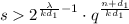
Thus if for some i, $\mathbf{z}_i-\mathbf{s}_i\mathbf{c}\ne \mathbf{0}$, we have a solution for ${R^{<n}}$-${\textsc {SIS}}_{k,d,\beta +sc}$. If we consider the function defined as $f(\mathbf{s}_1,\cdots ,\mathbf{s}_k)=\sum \limits _{i=1}^k \mathbf{a}_i'\mathbf{s}_i$, the domain size of this function is $(2s+1)^{kd_1}$, while the range is of size $q^{n+d_1-1}$. Because we set $s>2^{\lambda /(kd_1)-1}\cdot q^{(n+d_1-1)/(kd_1)}$, the size of the domain is greater than $2^{\lambda }\cdot q^{n+d_1-1}$. By Lemma 2.11, there is probability at least $1-2^{-\lambda }$ that there exists another such that

$$\mathbf{t}=\sum \limits _{i=1}^k \mathbf{a}_i'\mathbf{s}_i=\sum \limits _{i=1}^k \mathbf{a}_i'\mathbf{s}_i'.$$

Since it is perfectly indistinguishable whether $\mathbf{s}_1,\ldots ,\mathbf{s}_k$ or $\mathbf{s}_1',\ldots ,\mathbf{s}_k'$ were used in creating $\mathbf{t}$ (because both of them have the same posterior probability of having been chosen), the probability of the oracle outputting $\mathbf{z}_1,\ldots ,\mathbf{z}_k,\mathbf{c}$ such that$\mathbf{z}_i-\mathbf{s}_i\mathbf{c}\bmod \mathbf{f}=\mathbf{0}$ is exactly the same if $\mathbf{t}$ were generated as in the reduction, but then after the adversary produced his output, the preimage of $\mathbf{t}$ was chosen at random among all the valid choices. We will now show that $\mathbf{z}_i-\mathbf{s}_i\mathbf{c}$ can only equal $\mathbf{0}$ for all i for at most one of these choices.

If $(\mathbf{s}_1,\ldots ,\mathbf{s}_k)\ne (\mathbf{s}_1',\ldots ,\mathbf{s}_k')$, then there should be at least one $\mathbf{s}_i\ne \mathbf{s}_i'$. For this i, suppose that $\mathbf{z}_i-\mathbf{s}_i\mathbf{c}=\mathbf{0}=\mathbf{z}_i-\mathbf{s}'_i\mathbf{c}$. This implies that $(\mathbf{s}_i-\mathbf{s}'_i)\mathbf{c}=\mathbf{0}.$ Since $\mathbb {Z}_q[\mathbf{x}]$ is an integral domain, this can only happen if either $\mathbf{c}=\mathbf{0}$ or if $\mathbf{s}_i=\mathbf{s}_i'$. This is a contradiction. Therefore with probability at least 1/2, some $\mathbf{z}_i-\mathbf{s}_i\mathbf{c}\ne \mathbf{0}$.    $\square$

4 The Signature Scheme

We now formally describe our scheme via secret key generation, public key generation, signing, and verification algorithms.

The fixed, public parameters in our scheme are stated below. The values $n, k, q, s, d_1,d_2, c$ are intuitively related to the parametrization of the ${R^{<n}}$-${\textsc {SIS}}$ problem, with the standard deviation $\sigma$ being related to the parameter $\beta$. We furthermore define a cryptographic function $\text {H}$ whose range is the set C which consists of bounded-degree polynomials with small $\ell _1$ norms.

In Fig. 1, we give some sample parameters with which our scheme can be instantiated. For this, we use the reduction from breaking the signature scheme to the $\mathbf{f}$-${\textsc {SIS}}$ problem that is given in the next section. In that section we show that breaking the scheme implies solving the $\mathbf{f}$-${\textsc {SIS}}_{k,q,\beta }$ problem for $\beta =2sc+10\sigma$. Even though there is a reduction from every $\mathbf{f}$ whose degree is between $d_2$ and n, we instantiate the security based on the hardness of the $\mathbf{f}$-${\textsc {SIS}}$ problem for $\mathbf{f}$ whose degree is close to n. Of course if one wants to be more conservative, one could set the parameters so that the scheme is even secure in practice for polynomials whose degrees are closer to $d_2$.

To set the concrete parameters, we use the standard notion of the Hermite factor defined in [GN08] and the explanation for how to approximate it for the ${\textsc {SIS}}$ problem given in [MR08].

The key generation algorithm generates and , and then outputs $(\mathbf{a}_1,\ldots ,\mathbf{a}_k,\mathbf{t}=\sum \limits _{i=1}^{k}\mathbf{a}_i\mathbf{s}_i)$ as the public key. This is, in fact, an instance of the inhomogeneous ${R^{<n}}$-${\textsc {SIS}}$ problem from Definition 3.3.

Fig. 1.

Sample parameters for the signature scheme

To generate a signature of $\mu$, the signer selects “masking” variables $\mathbf{y}_i$ from a particular distribution, computes $\mathbf{c}=\text {H}(\sum \mathbf{a}_i\mathbf{y}_i,\mu )$, and then creates $\mathbf{z}_i=\mathbf{s}_i\mathbf{c}+\mathbf{y}_i$. By the way the parameters were set, each $\mathbf{z}_i$ is in . Thus the concatenation of the k vectors $\mathbf{z}=(\mathbf{z}_1~|~\ldots ~|\mathbf{z}_k)$ can be thought of as a vector in $\mathbb {Z}^{kd_2}$. If we similarly define the vector $\mathbf{s}=(\mathbf{s}_1\mathbf{c}~|~\ldots ,\mathbf{s}_k\mathbf{c})\in \mathbb {Z}^{kd_2}$, then we can see that the vector $\mathbf{z}$ is distributed according to the discrete Gaussian distribution $D^{kd_2}_{\mathbf{s},\sigma }$. To get rid of the dependence on $\mathbf{s}$, we use the rejection sampling procedure from [Lyu12] by running the RejectionSample algorithm. By the way the parameters are set, there is a 1/3 probability that the signature will be output, and a 2/3 chance that the signing procedure will need to be restarted. After some $(\mathbf{z}_1,\ldots ,\mathbf{z}_k)$ eventually passes the rejection sampling procedure, its distribution will be exactly $D_\sigma ^{kd_2}$.

Because the distribution is being sampled from $\mathbb {Z}^{kn}$, which is an orthogonal lattice, each coefficient of $\mathbf{z}_i$ is distributed according to $D^1_\sigma$. Thus, by Lemma 2.6, the probability that some coefficient is larger than $5\sigma$ in absolute value is less than $2e^{-25/2} < 2^{-17}$. For simplicity, we would like to make sure that all $\mathbf{z}_i$ are small, and so we check that each of their coefficients is less than $5\sigma$. The probability that all $kd_2$ positions are less than $5\sigma$ is at least $1-kd_2\cdot 2^{-17}$. In our sample instantiation, $kd_2<2^{13}$, and thus the probability that this check is passed is greater than 15/16. So with probabilty at most 1/16, the procedure gets restarted. The signing algorithm finally outputs $(\mathbf{z}_1,\ldots ,\mathbf{z}_k,\mathbf{c})$.

The verification algorithm looks at the signature $(\mathbf{z}_1,\ldots ,\mathbf{z}_k,\mathbf{c})$ and accepts if and only if all the coefficients of the $\mathbf{z}_i$ are less than $5\sigma$ and $\mathbf{c}=\text {H}\left( \sum \limits _{i=1}^{k}\mathbf{a}_i\mathbf{z}_i-\mathbf{t}\mathbf{c},\mu \right)$.

4.1 Security

The main result of this section is a reduction from solving the $R^{<n}$-${\textsc {SIS}}_{k,d_2,2sc+10\sigma }$ problem to forging the signature scheme. We first show how one can simulate the signing algorithm without knowing the secret key $\mathbf{s}_1,\ldots ,\mathbf{s}_k$ by programming the random oracle (Lemma 4.1).

We then show in Theorem 4.2 that an adversary who breaks the signature scheme that uses the signing algorithm from Lemma 4.1 can be used to solve either the $R^{<n}$-${\textsc {SIS}}$ problem from Definition 3.1 or the one from Definition 3.3. By Lemma 3.4, this implies that the adversary can be used to solve the problem from Definition 3.1, and therefore any instance of the $\mathbf{f}$-${\textsc {SIS}}$ problem for $\mathbf{f}$ of degree between $d_2$ and n. The latter then allows one to solve worst-case lattice problems in the ring $\mathbb {Z}[\mathbf{x}]/\langle \mathbf{f}\rangle$.

Lemma 4.1

Suppose that the random oracle $\text {H}$ is already programmed on v values. Then the statistical distance between the output of the signing procedure and the following Hybrid signing algorithm, which does not take any secret keys $\mathbf{s}_i$ as inputs, is at most $2^{-95}+v(\sqrt{2\pi }\sigma -1)^{-d_2}$.

Proof

We first define another intermediate signing hybrid algorithm named HybridSign$'$.

The difference between the real signing procedure and HybridSign$'$ is that the value of

$$\mathbf{c}=\text {H}\left( \sum \limits _{i=1}^{k}\mathbf{a}_i\mathbf{z}_i-\mathbf{t}\mathbf{c},\mu \right) =\text {H}\left( \sum \limits _{i=1}^{k}\mathbf{a}_i\mathbf{y}_i,\mu \right) $$

gets set uniformly at random in HybridSign$'$, whereas in the real signature scheme, $\text {H}$ would first check whether $\text {H}$ was already evaluated on $\left( \sum \limits _{i=1}^{k}\mathbf{a}_i\mathbf{y}_i,\mu \right)$ and only assign it a random value if it wasn’t. Therefore HybridSign$'$ will differ from the real scheme in the case that the value of $\sum \limits _{i=1}^{k}\mathbf{a}_i\mathbf{y}_i$ collides with one of the already-queried values.

For any $\mathbf{w}$,

where the last inequality holds because there is at most one possible $\mathbf{z}_1$ that satisfies this equation (because $\mathbb {Z}_q[\mathbf{x}]$ is an integral domain) and because the likeliest element in the discrete Gaussian distribution is $\mathbf{0}$ which has probability less than $(\sqrt{2\pi }\sigma -1)^{-n}$. Thus if there were already v values of the random oracle that were set, there is less than a $v\cdot (\sqrt{2\pi }\sigma -1)^{-d_2}$ probability that there would be a collision. In our sample instantiation, for example, $\sigma$ is approximately $2^{25}$ and $d_2>1200$, and so this probability is extremely small.

We now compare HybridSign$'$ with Hybrid 2. Lemma 2.7 states that the distribution of the eventual value of $(\mathbf{z}_1,\ldots ,\mathbf{z}_k,\mathbf{c})$ after the first 5 steps of HybridSign$'$ is within statistical distance $2^{-95}$ of the distribution of $(\mathbf{z}_1,\ldots ,\mathbf{z}_k,\mathbf{c})$ after two steps of HybridSign. Since the rest of the steps in both hybrids is identical, their statistical distance is at most $2^{-95}$. Thus the statistical distance of the distributions of the output of the real signing algorithm and HybridSign is $2^{-95}+(\sqrt{2\pi }\sigma -1)^{-d_2}$.   $\square$

Theorem 4.2

Suppose there exists an adversary who makes a total of t queries to the Signing hybrid in Lemma 4.1 and the random oracle H during his attack and succeeds in forging with probability $\delta$. Then there is an algorithm with the same time complexity that solves either the $R^{<n}$-${\textsc {SIS}}_{k,d_1,d_2,s,2c,10\sigma }$ problem or the $R^{<n}$-${\textsc {SIS}}_{k,d_2,10\sigma }$ problem with probability at least

$$\begin{aligned} \frac{1}{2}\cdot \left( \delta -\frac{1}{|C|}\right) \left( \frac{\delta -1/|C|}{t}-\frac{1}{|C|}\right) . \end{aligned}$$

Proof

Let $(\mathbf{a}_1,\ldots ,\mathbf{a}_k,\mathbf{t})$ be an instance of the ${R^{<n}}$-${\textsc {SIS}}_{k,d_1,d_2,s,2c,10\sigma }$ problem and $(\mathbf{a}_1',\ldots ,\mathbf{a}_k')$ be an instance of the ${R^{<n}}$-${\textsc {SIS}}_{k,d_2,10\sigma }$ problem. If we choose and compute $\mathbf{t}'=\sum \mathbf{a}_i'\mathbf{s}_i'$, then the distribution of $(\mathbf{a}_1,\ldots ,\mathbf{a}_k,\mathbf{t})$ is exactly the same as that of $(\mathbf{a}_1',\ldots ,\mathbf{a}_k',\mathbf{t}')$. The simulator then chooses one of those two sets at random and declares it as the public key of the signature scheme. If the adversary produces a forgery on a new message, then we will show that he will solve an instance of the $R^{<n}$-${\textsc {SIS}}_{k,d_1,d_2,s,2c,10\sigma }$ problem. If he produces a signature of a message he has already seen, then he will solve the $R^{<n}$-${\textsc {SIS}}_{k,d_2,10\sigma }$ problem. The simulator’s hope is therefore that if he gives the adversary the instance $(\mathbf{a}_1,\ldots ,\mathbf{a}_k,\mathbf{t})$, the adversary will forge a signature on a new message, whereas if the simulator gives $(\mathbf{a}_1',\ldots ,\mathbf{a}_k',\mathbf{t}')$, the adversary will forge on a message he has already seen. It’s easy to see that this lowers the success probability of the simulator by a factor of 2.

For simplicity, we will now refer to the public key as $(\mathbf{a}_1,\ldots ,\mathbf{a}_k,\mathbf{t})$. During the attack, the adversary may interact with the Simulator in one of three ways. He may ask for a signature of a message $\mu '$ for which the Simulator will use Hybrid 2, or query the hash function $\text {H}$ on any element in $\{0,1\}^*$, or produce a forgery $\mu$. If the adversary asks for a signature of $\mu$, the Simulator simply returns the output of Hybrid 2. If the adversary queries $\text {H}$ on some value, then the Simulator first checks if that value was already assigned and returns it, or otherwise just chooses a random element $\mathbf{c}\in C$ and programs it to be the output of $\text {H}$ on the adversary’s input.

If the adversary comes up with a signature $(\mathbf{z}_1,\ldots ,\mathbf{z}_k,\mathbf{c})$ for a message $\mu$, then this signature satisfies the equality $\mathbf{c}=\text {H}\left( \sum \limits _{i=1}^{k}\mathbf{a}_i\mathbf{z}_i-\mathbf{t}\mathbf{c},\mu \right)$. If the value for $\text {H}\left( \sum \limits _{i=1}^{k}\mathbf{a}_i\mathbf{z}_i-\mathbf{t}\mathbf{c},\mu \right)$ has never been programmed during a signing query or a random oracle query, then the adversary has only a 1/|C| chance of guessing the $\mathbf{c}$ that equals to $\text {H}\left( \sum \limits _{i=1}^{k}\mathbf{a}_i\mathbf{z}_i-\mathbf{t}\mathbf{c},\mu \right)$. So we will assume that the value for $\text {H}\left( \sum \limits _{i=1}^{k}\mathbf{a}_i\mathbf{z}_i-\mathbf{t}\mathbf{c},\mu \right)$ has already been set.

We will first handle the case where it has been set during a signing query. In this case, the simulator already gave a signature $(\mathbf{z}_1',\ldots ,\mathbf{z}_k',\mathbf{c})$ for the message $\mu$. In order for $(\mathbf{z}_1,\ldots ,\mathbf{z}_k,\mathbf{c})$ to be a valid forgery for $\mu$, some $\mathbf{z}_i$ must be different from $\mathbf{z}_i'$. The adversary’s forgery therefore implies that

$$\sum \limits _{i=1}^{k}\mathbf{a}_i\mathbf{z}_i-\mathbf{t}\mathbf{c}=\sum \limits _{i=1}^{k}\mathbf{a}_i\mathbf{z}_i'-\mathbf{t}\mathbf{c},$$

and therefore

$$\sum \limits _{i=1}^{k}\mathbf{a}_i(\mathbf{z}_i-\mathbf{z}_i')=\mathbf{0}$$

and at least for one i, $\mathbf{z}_i\ne \mathbf{z}_i'$. Since all $\Vert \mathbf{z}_i-\mathbf{z}_i'\Vert _\infty \le 10\sigma$ and $\deg (\mathbf{z}_i-\mathbf{z}_i')\le d_2$, they form a solution to the $R^{<n}$-${\textsc {SIS}}_{n,q,d_2,10\sigma }$ problem.

We now move to the case where the adversary constructs a signature for a message he has not yet seen. If the adversary comes up with a valid forgery $(\mathbf{z}_1,\ldots ,\mathbf{z}_k,\mathbf{c})$ for a new message $\mu$, then $\Vert \mathbf{z}_i\Vert _\infty \le 5\sigma$ and $\mathbf{c}=\text {H}\left( \sum \limits _{i=1}^{k}\mathbf{a}_i\mathbf{z}_i-\mathbf{t}\mathbf{c},\mu \right)$. As before, if the adversary never queried $\text {H}$ on $\left( \sum \limits _{i=1}^{k}\mathbf{a}_i\mathbf{z}_i-\mathbf{t}\mathbf{c},\mu \right)$, then he only has at most a 1/|C| chance of producing such a forgery. Thus let’s assume that the adversary did make such a “winning” query. We then “rewind” the adversary by rerunning him with the same random coins and responding to all the random oracle queries (both his and the ones used in the signing) the same way as before until the “winning” query. Starting from the “winning” query, however, we select uniformly random responses to all random oracle queries. Let $\mathbf{c}'$ be the new response to the “winning” query. By the General Forking Lemma of Bellare and Neven [BN06, Lemma 1], the probability that $\mathbf{c}\ne \mathbf{c}'$ and the adversary again forges on the “winning” query is at least

$$\begin{aligned} \left( \delta -\frac{1}{|C|}\right) \left( \frac{\delta -1/|C|}{t}-\frac{1}{|C|}\right) . \end{aligned}$$

With the above probability, then, the Simulator obtains another equation $\mathbf{c}'=\text {H}\left( \sum \limits _{i=1}^{k}\mathbf{a}_i\mathbf{z}_i'-\mathbf{t}\mathbf{c}',\mu \right)$ where $\sum \limits _{i=1}^{k}\mathbf{a}_i\mathbf{z}_i'-\mathbf{t}\mathbf{c}'=\sum \limits _{i=1}^{k}\mathbf{a}_i\mathbf{z}_i-\mathbf{t}\mathbf{c}$ because the query was the same in both runs of the adversary. Therefore

$$\sum \limits _{i=1}^{k}\mathbf{a}_i(\mathbf{z}-\mathbf{z}_i')=\mathbf{t}(\mathbf{c}-\mathbf{c}')$$

and so $(\mathbf{z}_1-\mathbf{z}_1',\ldots ,\mathbf{z}_k-\mathbf{z}_k',\mathbf{c}-\mathbf{c}')$ is a solution to the instance $(\mathbf{a}_1,\ldots ,\mathbf{a}_k,\mathbf{t})$ of the $R^{<n}$-${\textsc {SIS}}_{k,d_1,d_2,s,2c,10\sigma }$ problem.    $\square$

Putting Theorem 4.2, Lemmas 3.4, and 4.1 together, we see that if the signature scheme parameters satisfy the pre-conditions on the public parameters in Lemma 3.4, then an adversary who breaks the signature scheme either solves the $R^{<n}$-${\textsc {SIS}}_{k,d_2,10\sigma }$ problem or the $R^{<n}$-${\textsc {SIS}}_{k,d_2,2sc+10\sigma }$ problem (the latter is a strictly weaker problem). This implies that an adversary who breaks the signature scheme can be used to break the $\mathbf{f}$-${\textsc {SIS}}_{k,q,2sc+10\sigma }$ problem for any polynomial $\mathbf{f}$ of degree between $d_2$ and n. By Theorem 2.3, this in turn gives a connection between breaking the signature scheme and finding short vectors for any lattice in any polynomial ring $\mathbb {Z}[\mathbf{x}]/\langle \mathbf{f}\rangle$ where the degree of $\mathbf{f}$ is between $d_2$ and n.

References

Albrecht, M., Bai, S., Ducas, L.: A subfield lattice attack on overstretched NTRU assumptions: cryptanalysis of some FHE and graded encoding schemes. IACR Cryptology ePrint Archive 2016, p. 127 (2016)
Ajtai, M.: Generating hard instances of lattice problems (extended abstract). In: STOC, pp. 99–108 (1996)
Bernstein, D.J., Chuengsatiansup, C., Lange, T., van Vredendaal, C.: NTRU prime. Cryptology ePrint Archive, Report 2016/461 (2016). http://eprint.iacr.org/
Bellare, M., Neven, G.: Multi-signatures in the plain public-key model and a general forking lemma. In: ACM Conference on Computer and Communications Security, pp. 390–399 (2006)
Jean-François Biasse and Fang Song. Efficient quantum algorithms for computing class groups and solving the principal ideal problem in arbitrary degree number fields. In: SODA, pp. 893–902 (2016)
Cramer, R., Ducas, L., Peikert, C., Regev, O.: Recovering short generators of principal ideals in cyclotomic rings. In: Fischlin, M., Coron, J.-S. (eds.) EUROCRYPT 2016. LNCS, vol. 9666, pp. 559–585. Springer, Heidelberg (2016). doi:10.1007/978-3-662-49896-5_20
Campbell, P., Groves, M., Shepherd, D.: Soliloquy: a cautionary tale. In: ETSI/IQC 2nd Quantum-Safe Crypto Workshop (2014)
Cheon, J.H., Jeong, J., Lee, C.: An algorithm for NTRU problems and cryptanalysis of the GGH multilinear map without an encoding of zero. IACR Cryptology ePrint Archive (2016)
Ducas, L., Durmus, A., Lepoint, T., Lyubashevsky, V.: Lattice signatures and bimodal gaussians. In: Canetti, R., Garay, J.A. (eds.) CRYPTO 2013. LNCS, vol. 8042, pp. 40–56. Springer, Heidelberg (2013). doi:10.1007/978-3-642-40041-4_3
Eisenträger, K., Hallgren, S., Kitaev, A.Y., Song, F.: A quantum algorithm for computing the unit group of an arbitrary degree number field. In: STOC (2014)
Güneysu, T., Lyubashevsky, V., Pöppelmann, T.: Practical lattice-based cryptography: a signature scheme for embedded systems. In: CHES, pp. 530–547 (2012)
Gama, N., Nguyen, P.Q.: Predicting lattice reduction. In: Smart, N. (ed.) EUROCRYPT 2008. LNCS, vol. 4965, pp. 31–51. Springer, Heidelberg (2008). doi:10.1007/978-3-540-78967-3_3
Gentry, C., Szydlo, M.: Cryptanalysis of the revised NTRU signature scheme. In: Knudsen, L.R. (ed.) EUROCRYPT 2002. LNCS, vol. 2332, pp. 299–320. Springer, Heidelberg (2002). doi:10.1007/3-540-46035-7_20
Lyubashevsky, V., Micciancio, D.: Generalized compact knapsacks are collision resistant. In: Bugliesi, M., Preneel, B., Sassone, V., Wegener, I. (eds.) ICALP 2006. LNCS, vol. 4052, pp. 144–155. Springer, Heidelberg (2006). doi:10.1007/11787006_13
Lyubashevsky, V., Peikert, C.: On ideal lattices, learning with errors over rings. J. ACM 60(6), 43 (2013). Preliminary version appeared in EUROCRYPT 2010
Lyubashevsky, V.: Fiat-Shamir with aborts: applications to lattice and factoring-based signatures. In: Matsui, M. (ed.) ASIACRYPT 2009. LNCS, vol. 5912, pp. 598–616. Springer, Heidelberg (2009). doi:10.1007/978-3-642-10366-7_35
Lyubashevsky, V.: Lattice signatures without trapdoors. In: Pointcheval, D., Johansson, T. (eds.) EUROCRYPT 2012. LNCS, vol. 7237, pp. 738–755. Springer, Heidelberg (2012). doi:10.1007/978-3-642-29011-4_43
Micciancio, D., Regev, O.: Lattice-based cryptography. In: Bernstein, D.J., Buchmann, J., Dahmen, E. (eds.) Post-Quantum Cryptography, pp. 147–191. Springer, Heidelberg (2009)
Peikert, C., Rosen, A.: Efficient collision-resistant hashing from worst-case assumptions on cyclic lattices. In: Halevi, S., Rabin, T. (eds.) TCC 2006. LNCS, vol. 3876, pp. 145–166. Springer, Heidelberg (2006). doi:10.1007/11681878_8
Peikert, C., Rosen, A.: Lattices that admit logarithmic worst-case to average-case connection factors. In: STOC, pp. 478–487 (2007)
Stehlé, D., Steinfeld, R., Tanaka, K., Xagawa, K.: Efficient public key encryption based on ideal lattices. In: Matsui, M. (ed.) ASIACRYPT 2009. LNCS, vol. 5912, pp. 617–635. Springer, Heidelberg (2009). doi:10.1007/978-3-642-10366-7_36
Author information
Authors and Affiliations
Corresponding author
Editor information
Editors and Affiliations
Rights and permissions
Copyright information
© 2016 International Association for Cryptologic Research
About this paper
Cite this paper
Lyubashevsky, V. (2016). Digital Signatures Based on the Hardness of Ideal Lattice Problems in All Rings. In: Cheon, J., Takagi, T. (eds) Advances in Cryptology – ASIACRYPT 2016. ASIACRYPT 2016. Lecture Notes in Computer Science(), vol 10032. Springer, Berlin, Heidelberg. https://doi.org/10.1007/978-3-662-53890-6_7
Download citation
DOI: https://doi.org/10.1007/978-3-662-53890-6_7
Published:
Publisher Name: Springer, Berlin, Heidelberg
Print ISBN: 978-3-662-53889-0
Online ISBN: 978-3-662-53890-6
eBook Packages: Computer ScienceComputer Science (R0)