Sub-linear Lattice-Based Zero-Knowledge Arguments for Arithmetic Circuits

Abstract

We propose the first zero-knowledge argument with sub-linear communication complexity for arithmetic circuit satisfiability over a prime ${p}$ whose security is based on the hardness of the short integer solution (SIS) problem. For a circuit with ${N}$ gates, the communication complexity of our protocol is $O\left( \sqrt{{N}{\lambda }\log ^3{{N}}}\right)$, where ${\lambda }$ is the security parameter. A key component of our construction is a surprisingly simple zero-knowledge proof for pre-images of linear relations whose amortized communication complexity depends only logarithmically on the number of relations being proved. This latter protocol is a substantial improvement, both theoretically and in practice, over the previous results in this line of research of Damgård et al. (CRYPTO 2012), Baum et al. (CRYPTO 2016), Cramer et al. (EUROCRYPT 2017) and del Pino and Lyubashevsky (CRYPTO 2017), and we believe it to be of independent interest.

Jonathan Bootle, Andrea Cerulli and Jens Groth were supported by funding from the European Research Council under the European Union’s Seventh Framework Programme (FP/2007-2013)/ERC Grant Agreement n. 307937. Rafael del Pino and Vadim Lyubashevsky were supported in part by the SNSF ERC Transfer Starting Grant CRETP2-166734-FELICITY. Carsten Baum acknowledges support by the BIU Center for Research in Applied Cryptography and Cyber Security in conjunction with the Israel National Cyber Bureau in the Prime Ministers Office.

1 Introduction

Zero-knowledge proofs and arguments are used throughout cryptography as a key ingredient to ensure security in complex protocols. They form an important part of applications such as authentication protocols, electronic voting systems, encryption primitives, multi-party computation schemes, and verifiable computation protocols. Therefore, designing zero-knowledge protocols with strong security and high efficiency is of the utmost importance.

A zero-knowledge argument allows a prover to convince a verifier that a particular statement is true, without the prover revealing any other information that she knows about the statement. Statements are of the form ${u}\in {\mathcal {L}}$, where ${\mathcal {L}}$ is a language in NP. We call ${w}$ a witness for statement ${u}$ if $({u},{w})\in {R}$, where ${R}$ is a polynomial time decidable binary relation associated with ${\mathcal {L}}$. Zero-knowledge arguments must be complete, sound and zero-knowledge.

• Completeness: A prover with witness ${w}$ for ${u}\in {\mathcal {L}}$ can convince the verifier.

• Soundness: A prover cannot convince the verifier when ${u}\notin {\mathcal {L}}$.

• Zero-knowledge: The interaction should not reveal anything to the verifier except that ${u}\in {\mathcal {L}}$. In particular, it should not reveal the prover’s witness ${w}$.

We wish to design a zero-knowledge argument based on the short integer solution (SIS) assumption. Lattice problems appear to resist quantum attacks, and possess attractive worst-case to average-case reductions, in stark contrast with number theoretic assumptions such as the hardness of factoring or computing discrete logarithms. Moreover, using SIS (and the even more efficient Ring-SIS) yields better computational efficiency, which is a significant bottleneck in many zero-knowledge arguments.

1.1 Our Contributions

We provide an honest verifier zero-knowledge argument for arithmetic circuit satisfiability over ${\mathbb {Z}}_{p}$, for an arbitrary prime ${p}$. Our argument is based on the SIS assumption [Ajt96, MR04], which is conjectured to be secure even against a quantum adversary. Our argument has an expected constant number of moves and sub-linear communication complexity, as shown in Table 1. Moreover, it achieves small soundness error in a single protocol execution. Moreover, both the prover and verifier have quasi-linear computational complexity in the amount of computation it would require to evaluate the arithmetic circuit directly. The argument therefore improves on the state-of-the-art in communication complexity for lattice proof systems and is efficient on all performance parameters.

Table 1. Performance of our zero-knowledge argument for arithmetic circuit satisfiability. Here ${N}$ is the number of gates in the arithmetic circuit, and ${\lambda }$ is the security parameter.

Techniques. We draw inspiration from the discrete logarithm based arithmetic circuit satisfiability argument of Bootle et al. [BCC+16], which requires 5 moves and has square root communication complexity in the number of multiplication gates. In their argument the prover commits to all the wires using homomorphic commitments, and embeds the wire values into a polynomial that verifies products and linear relations simultaneously, avoiding the cost for addition gates.

Almost all parts of the original arguments adapt seamlessly to the SIS setting, except for two important issues:

• To achieve sub-linear communication, we need a technique for proving knowledge of commitment openings in sub-linear space.

• Due to the new algebraic setting, we require new techniques for achieving negligible soundness in a single run of the protocol.

The first of these issues has been an open problem in a fairly active area of research, and we sketch our solution below.

Proof of Knowledge. Suppose that we have a linear relation

$$\begin{aligned} {\varvec{A}} {\varvec{s}} = {\varvec{t}}\bmod \,{q}, \end{aligned}$$

(1)

where ${\varvec{A}}\in {\mathbb {Z}}_{q}^{{r}\times {v}},{\varvec{t}}\in {\mathbb {Z}}_{q}^{{r}}$ are public and ${\varvec{s}}\in {\mathbb {Z}}_{q}^{v}$ is a vector with small coefficients, and we want to give a zero-knowledge proof of knowledge of an $\bar{{\varvec{s}}}$ with small coefficients (the coefficients of $\bar{{\varvec{s}}}$ may be larger than those of ${\varvec{s}}$) that satisfies

$$\begin{aligned} {\varvec{A}}\bar{{\varvec{s}}}={\varvec{t}}\bmod \,{q}. \end{aligned}$$

(2)

We do not currently know of any an efficient linear-communication protocol for proving knowledge of a single relation of the above form in a direct way. There are protocols, however, that allow for proofs of many such relations for the same ${\varvec{A}}$ but different ${\varvec{s}}_i$ (and thus different ${\varvec{t}}_i$) in linear amortized complexity. We will mention these previous works in more detail in Sect. 1.2.

In this work, we give a protocol for proving (1) where the proof length is a factor $\frac{{\lambda }}{{\ell }}\cdot O(\log {{v}{\ell }{\lambda }})$ larger than the total bit-length of ${\ell }$ pre-images ${\varvec{s}}_1,\ldots ,{\varvec{s}}_{\ell }$ of the relations, where ${\lambda }$ is the security parameter. More specifically, to prove knowledge of ${\ell }$ pre-images ${\varvec{s}}_1,\ldots ,{\varvec{s}}_{\ell }$ whose coefficients have $\log {s}$ bits each, the prover needs to send ${\lambda }$ vectors in ${\mathbb {Z}}_{q}^{v}$ whose coefficients require $O(\log {{v}{\ell }{\lambda }s})$ bits to represent. Ignoring logarithmic terms, our proof essentially requires a fixed-size proof regardless of the number of relations being proved. The previously best results had proofs that were at least linear in the total size of the pre-images.

Surprisingly, the proof of knowledge protocol turns out to just be a parallel repetition of ${\lambda }$ copies of the ZKPoK implicit in the signing protocol from [Lyu12]. In particular, if we write the ${\ell }$ relations as ${\varvec{A}}{\varvec{S}} = {\varvec{T}}\bmod \,{q}$, where ${\varvec{S}}\in {\mathbb {Z}}_{q}^{{v}\times {\ell }}$, then the protocol begins with the prover selecting a “masking” value ${\varvec{Y}}$ with small coefficients and sending ${\varvec{W}} = {\varvec{A}}{\varvec{Y}}\bmod \,{q}$. The verifier then picks a random challenge matrix ${\varvec{C}}\in \{0,1\}^{{\ell }\times ({\lambda }+ 2)}$, and sends it to the prover. The prover computes ${\varvec{Z}} = {\varvec{S}}{\varvec{C}}+{\varvec{Y}}$ and performs a rejection sampling step in order to make the distribution of ${\varvec{Z}}$ independent from ${\varvec{S}}$, and if it passes, sends ${\varvec{Z}}$ to the verifier. The verifier checks that all columns comprising ${\varvec{Z}}$ have small norms and that ${\varvec{A}}{\varvec{Z}} = {\varvec{T}}{\varvec{C}} + {\varvec{W}}\bmod \,{q}$. This protocol can be shown to be zero-knowledge using exactly the same techniques as in [Lyu09, Lyu12].

To show that the protocol is a proof of knowledge, we make the following observation: if the prover succeeds with probability $\epsilon >2^{-{\lambda }}$, and she succeeded for a random ${\varvec{C}}$, then there is a probability of $\epsilon - 2^{-{\lambda }-2}$ that she would successfully answer another challenge ${\varvec{C}}'\ne {\varvec{C}}$ that is constructed such that all rows except the $i^{th}$ are the same as that of ${\varvec{C}}$, and the $i^{th}$ row is picked uniformly at random. This property follows from an averaging (or “heavy row”) type argument. The implication is that if the prover succeeds in time t with probability $\epsilon$, then the extractor can extract responses to two such commitments ${\varvec{C}},{\varvec{C}}'$ in expected time $O(t/\epsilon )$. Obtaining two responses ${\varvec{Z}},{\varvec{Z}}'$ for two such challenges allows the extractor to compute ${\varvec{A}}({\varvec{Z}}-{\varvec{Z}}')={\varvec{T}}({\varvec{C}}-{\varvec{C}}')$ where ${\varvec{C}}-{\varvec{C}}'$ is 0 everywhere except in row i. Since ${\varvec{C}}\ne {\varvec{C}}'$, this implies that some position in row i is $\pm 1$. If ${\varvec{t}}_i$ is the $i^{th}$ column of ${\varvec{T}}$ and ${\varvec{z}}_i$ is the $i^{th}$ column of ${\varvec{Z}}-{\varvec{Z}}'$, then we have a solution ${\varvec{A}}{\varvec{z}}_i=\pm {\varvec{t}}_i$. Repeating this extraction ${\ell }$ times, each time rewinding by fixing all rows in the challenge except for the $i^{th}$, results in an algorithm that runs in expected time $O({\ell }\cdot t/\epsilon )$, which is only a factor of ${\ell }$ larger than the expected running time of a successful prover.

In the case that we are proving (1) over the polynomial ring $\mathbb {Z}[X]/(X^{d}+1)$, the proof can be even shorter, as we can reduce the number of columns in ${\varvec{C}}$ to $\approx {\lambda }/\log {2{d}}$ because we can use challenges of the form $\pm X^i$ and prove the knowledge of $\bar{{\varvec{s}}}$ such that ${\varvec{A}}\bar{{\varvec{s}}}=2{\varvec{t}}$ using the observation from [BCK+14].

Commitment Scheme. Central to the main proof of proving circuit satisfiability is being able to commit to ${N}$ values in ${\mathbb {Z}}_{p}$ and giving a ZKPoK for the values such that the total size of the commitments and the proofs is sub-linear in ${N}$. For this, it is necessary to use a compressing commitment scheme – i.e. one in which we can commit to ${n}$ elements of ${\mathbb {Z}}_{p}$ in space less than ${n}$ elements. The scheme that we will use is the “classic” statistically-hiding commitment scheme based on the hardness of SIS that was already implicit in the original work of Ajtai [Ajt96]. The public randomness consists of two matrices ${\varvec{A}}\in {\mathbb {Z}}_{q}^{{r}\times 2{r}\log _{p}{{q}}},{\varvec{B}}\in {\mathbb {Z}}_{q}^{{r}\times {n}}$, and committing to a message string ${\varvec{s}}\in {\mathbb {Z}}_{p}^{n}$ where $p<q$ involves picking a random vector ${\varvec{r}}\in {\mathbb {Z}}_{p}^{2{r}\log _{p}{{q}}}$ and outputting the commitment ${\varvec{t}}={\varvec{A}}{\varvec{r}}+{\varvec{B}}{\varvec{s}}\bmod \,{q}$. Thus the commitment of ${n}$ elements of ${\mathbb {Z}}_{p}$ requires ${r}\log {{q}}$ bits. One can set the parameters such that ${n}=\mathsf {poly}({r})$ and the commitment scheme will still be computationally binding based on the worst-case hardness of approximating SIVP for all lattices of dimension ${r}$.

We now explain the intuition for putting together this commitment scheme with the zero-knowledge proof system we described above to produce a commitment to ${N}$ values in ${\mathbb {Z}}_{p}$ such that the total size of the commitments and the ZKPoK of the committed values is $O(\sqrt{{N}{\lambda }\log {{N}}})$. The idea is to create ${N}/{n}$ commitments (for some choice of ${n}$ which will be optimized later), with each one committing to ${n}$ values. Our motivation is that an arithmetic circuit over ${\mathbb {Z}}_{p}$ with ${N}$ gates has $3{N}$ wire values in ${\mathbb {Z}}_{p}$. Now, we can arrange all of the wire values in the circuit into, for example, a $3{N}/{n}\times {n}$ matrix over ${\mathbb {Z}}_{p}$, and make one homomorphic commitment to all of the elements in each row of the matrix. Then, we can employ techniques from [Gro09a, BCC+16], where checking arithmetic circuit satisfiability is reduced to checking linear-algebraic statements over committed matrices, using a homomorphic commitment scheme.

The total space requirement for these commitments is therefore $\frac{{N}}{{n}}\cdot {r}\log _{p}{{q}}$. We now have a linear equation of the form $\begin{bmatrix} {\varvec{A}}&{\varvec{B}} \end{bmatrix}\begin{bmatrix} {\varvec{R}} \\ {\varvec{S}}\end{bmatrix} = {\varvec{T}} \bmod \,{q}$. Using our new zero-knowledge proof, the communication complexity of proving the knowledge of a short $\begin{bmatrix} \bar{{\varvec{R}}} \\ \bar{{\varvec{S}}}\end{bmatrix}\in {\mathbb {Z}}_{q}^{({r}\log _{p}{{q}}+{n})\times {N}/{n}}$ such that $\begin{bmatrix} {\varvec{A}}&{\varvec{B}} \end{bmatrix}\begin{bmatrix} \bar{{\varvec{R}}} \\ \bar{{\varvec{S}}}\end{bmatrix} = {\varvec{T}} \bmod \,{q}$ requires sending ${\lambda }$ vectors of length ${r}\log _{p}{{q}}+{n}$ with coefficients requiring $O(\log {{N}{\lambda }{p}})$ bits, for a total bit-length of ${n}\cdot {\lambda }\cdot O(\log {{N}{\lambda }{p}})$. Combining the proof size with the commitment size results in a total bit-size of

$$\frac{{N}}{{n}}\cdot {r}\log {{q}} + {n}\cdot {\lambda }\cdot O(\log {{N}{\lambda }{p}}).$$

We minimize the above by setting ${n}=\sqrt{\frac{{N}{r}\log _{p}{{q}}}{{\lambda }\log {{N}{\lambda }{p}}}}$, which makes the size

$$O\left( \sqrt{{N}{r}{\lambda }(\log _{p}{{q}})(\log {{N}{\lambda }{p})}}\right) .$$

Based on the complexity of the best known algorithm against the SIS problem, one can set $\log {{q}},{r}=O(\log {{N}})$, thus making the proof size of order $O(\sqrt{{N}{\lambda }\log ^3{N}})$.

1.2 Related Work

Zero-knowledge proofs were invented by Goldwasser et al. [GMR85]. It is useful to distinguish between zero-knowledge proofs, with statistical soundness, and zero-knowledge arguments with computational soundness. The most efficient proofs have communication proportional to the size of the witness [IKOS07, KR08, GGI+15] and proofs cannot in general have communication that is smaller than the witness size unless surprising results about the complexity of solving SAT instances hold [GH98, GVW02]. Kilian [Kil92] showed that in contrast to proofs, zero-knowledge arguments can have very low communication complexity. His construction relied on the PCP theorem, and thus incurred a large computational cost.

Group theoretic zero-knowledge arguments. Schnorr [Sch91] and Guillou and Quisquater [GQ88] gave early examples of practical zero-knowledge arguments for concrete number theoretic problems. Extending Schnorr’s protocols, there have been many constructions of zero-knowledge arguments based on the discrete logarithm assumption, for instance [CD97, Gro09a]. The most efficient discrete logarithm based zero-knowledge arguments for arithmetic circuits are by Bootle et al. [BCC+16] and later optimised in [BBB+17], which have logarithmic communication complexity and require a linear number of exponentiations.

An exciting line of research [Gro10a, Lip12, BCCT12, GGPR13, BCCT13, PHGR13, Gro16] on succinct non-interactive arguments (SNARGs) has yielded pairing-based constructions where the arguments consist of a constant number of group elements. However, it can be shown that all SNARKs must rely on non-falsifiable knowledge extractor assumptions [GW11]. In contrast, since our argument is interactive, we do not need to rely on these strong assumptions.

Lattice-based zero-knowledge arguments. The first zero-knowledge proofs from lattice-based assumptions were aimed at lattice problems themselves. Goldreich and Goldwasser [GG98] presented constant round interactive zero knowledge proofs for the complements of the approximate Shortest Vector Problem (SVP) and the approximate Closest Vector Problem (CVP). Micciancio and Vadhan [MV03] later constructed statistical zero knowledge proofs for these problems which had efficient provers.

Stern’s protocol [Ste94] was one of the first zero-knowledge identification protocols to be based on a post-quantum assumption, namely, on the hardness of syndrome decoding for a random linear code, which is essentially proving (1) where ${q}=2$ and $\Vert {\varvec{s}}\Vert \ll \sqrt{{v}}$. The protocol achieves constant soundness error, and thus requires many parallel repetitions. Stern’s work prompted many variants and similar protocols. For example, [LNSW13] adapts the protocol for larger ${q}$, which implies proving knowledge of SIS solutions.

Another technique for creating zero-knowledge proofs is the “Fiat-Shamir with Aborts” approach [Lyu09, Gro10b, Lyu12]. When working over polynomial rings R, it gives a proof of knowledge of a vector $\bar{{\varvec{s}}}$ with small coefficients (though larger than those in ${\varvec{s}}$) and a ring element $\bar{c}$ with very small coefficients satisfying ${\varvec{A}} \bar{{\varvec{s}}}=\bar{c}{\varvec{t}}$ . As long as the ring R has many elements with small coefficients, such proofs are very efficient, producing soundness of $1-2^{-128}$ with just one iteration. While these proofs are good enough for constructing practical digital signatures (e.g. [GLP12, DDLL13, BG14]), commitment schemes with proofs of knowledge [BKLP15, BDOP16], and certain variants of verifiable encryption schemes [LN17], they prove less than what the honest prover knows. In many applications where zero-knowledge proofs are used, in particular those that need to take advantage of additive homomorphisms, the presence of the element $\bar{c}$ makes these kinds of “approximate” proofs too weak to be useful. As of today, we do not have any truly practical zero-knowledge proof systems that give a proof of (1).

The situation is more promising when one considers amortized proofs. The work of [BD10] uses MPC-in-the-head to prove knowledge of plaintexts for multiple Regev [Reg05] ciphertexts. Damgård and López-Alt [DL12] extend the [BD10] results to prove knowledge of plaintext in ${\mathbb {Z}}_{p}$, rather than bits, and provide a proof for the correctness of multiplications. Combining these together gives a zero-knowledge proof for the satisfiability of arithmetic circuits with linear communication in the circuit size.

Another idea for proving the relation in (1) is to use the above-mentioned “Fiat-Shamir with Aborts” protocol, but with challenges that come from the set $\{0,1\}$. The works of [BDLN16, CDXY17, dPL17] gave a series of improved protocols that were able to employ this technique in the amortized setting. Their proofs had a small polynomial “slack” (i.e. the ratio between the original committed ${\varvec{s}}$ and the extracted $\bar{{\varvec{s}}}$) and were of approximate linear size when the number of commitments was a couple of thousand. The schemes are considerably less efficient when one is proving fewer relations.

The amortized zero-knowledge proof in the current work improves on the above series of papers in two important ways. First, the number of relations necessary before the size of our proof is linear only in ${\lambda }$. But more importantly, if we have more than ${\lambda }$ relations, the communication complexity does not increase except for small logarithmic factors (i.e. the proof size becomes sub-linear).

Hash-based zero-knowledge arguments. Recently Bootle et al. [BCG+17] used error-correcting codes and linear-time collision-resistant hash functions to give proof systems for the satisfiability of an arithmetic circuit where the prover uses a linear number of field multiplications. Verification is even more efficient, requiring only a linear number of additions. While their proofs and arguments are asymptotically very efficient, they are not quite practical as their choices of error-correcting codes and hash functions involves very large constants.

An another effective way to construct efficient zero-knowledge proofs is to follow the so-called MPC-in-the-head paradigm of [IKOS07]. This approach proved itself to give very efficient constructions both theoretically and practically. Most notably, ZKBOO [GMO16] and subsequent optimisation ZKB++ [CDG+17] use hash functions to construct zero-knowledge arguments for the satisfiability of boolean circuits. Their communication complexity is linear in the circuit size, but the use of symmetric primitives gives good performances in practice. Ligero [AHIV17] provides another implementation of the MPC-in-the-head paradigm and used techniques similar to  [BCG+17] to construct sublinear arguments for arithmetic circuits.

2 Preliminaries

Algorithms in our schemes receive a security parameter ${\lambda }$ as input (sometimes implicitly) written in unary. The intuition is that the higher the security parameter, the lower the risk of the scheme being broken. Given two functions $f,g:\mathbb {N}\rightarrow [0,1]$ we write $f({\lambda })\approx g({\lambda })$ when $|f({\lambda })-g({\lambda })|={\lambda }^{-\omega (1)}$. We say that f is negligible when $f({\lambda })\approx 0$ and that f is overwhelming when $f({\lambda })\approx 1$. For any integer ${N}$, $[{N}]$ denotes the set $\{0,1,\ldots ,{N}-1\}$ of integers.

2.1 Notation

Throughout this paper we will consider a ring ${\mathcal {R}}$, which will be either ${\mathbb {Z}}$ or the polynomial ring ${\mathbb {Z}}[X]/(X^{d}+1)$ for ${d}$ some power of 2. We will denote elements of ${\mathcal {R}}$ by lowercase letters, (column) vectors over ${\mathcal {R}}$ in bold lowercase and matrices over ${\mathcal {R}}$ in bold uppercase. e.g. ${\varvec{A}} = \begin{bmatrix} {\varvec{a}}_1,\ldots ,{\varvec{a}}_{k}\end{bmatrix}\in {\mathcal {R}}^{l\times {k}}$ with ${\varvec{a}}_i=(a_{i1},\ldots ,a_{im})^T\in {\mathcal {R}}^l$. We will consider the norm of elements in ${\mathcal {R}}$ to be $||a||{_{2}}=|a|$ if $a\in {\mathbb {Z}}$, and if $a=\sum a_iX^i\in {\mathbb {Z}}[X]/(X^{d}+1)$. We extend the notation to vectors and matrices , . We will also consider the quotient ring ${\mathcal {R}}_{q}= {\mathcal {R}}/{q}{\mathcal {R}}$ for odd ${q}$. In the quotient ring, the norm of an element ${\mathcal {R}}_{q}$ will be the norm of its unique representative ${\mathcal {R}}$ with coefficients in $\left[ -\frac{{q}-1}{2},\frac{{q}-1}{2} \right]$.

We will also consider the operator norm of matrices over ${\mathcal {R}}$ defined as .

Probability Distributions. Let $\mathcal {D}$ denote a distribution over some set. Then, $d \leftarrow \mathcal {D}$ means that d was sampled from the distribution $\mathcal {D}$. If we write for some finite set S without a specified distribution this means that d was sampled uniformly random from S. We let $\varDelta (X,Y)$ indicate the statistical distance between two distributions X, Y. Define the function $\rho _\sigma (x) = \exp \left( \frac{-x^2}{2\sigma ^2}\right)$ and the discrete Gaussian distribution over the integers, $D_\sigma$, as

$$\begin{aligned} D_\sigma (x)=\frac{\rho (x)}{\rho ({\mathbb {Z}})} \text { where } \rho ({\mathbb {Z}})=\sum \limits _{v\in {\mathbb {Z}}} \rho (v). \end{aligned}$$

We will write ${\varvec{X}}\leftarrow D_\sigma ^{{r}\times m}$ to mean that every coefficient of the matrix ${\varvec{X}}$ is distributed according to $D_\sigma$.

Using the tail bounds for the 0-centered discrete Gaussian distribution (cf. [Ban93]), we can show that for any $\sigma >0$ the norm of $\,x \leftarrow D_{\sigma }$ can be upper-bounded using $\sigma$. Namely, for any $k>0$ it holds that

(3)

and when ${\varvec{x}}$ is drawn from $D_\sigma ^{r}$, we have

(4)

We will abuse the notation $x\leftarrow D_\sigma$ when $x\in {\mathbb {Z}}[X]/(X^{d}+1)$ to denote the distribution in which each coefficient of x is taken from $D_\sigma$. It is clear that in this case $||x||{_{2}}$ can be bounded using Eq. 4 with ${d}$ instead of ${r}$.

2.2 Lattice-Based Commitment Schemes

A commitment scheme allows a sender to create commitments to secret values, which she might then decide to reveal later. The main properties of commitment schemes are hiding and binding. Hiding guarantees that commitments do not leak information about the committed values, while binding guarantees that the sender cannot change her mind and open commitments to different values.

Formally, a non-interactive commitment scheme is a pair of probabilistic polynomial-time algorithms $({\mathrm {Gen}}, {\mathrm {Com}})$. The setup algorithm $ck\leftarrow \mathrm {Gen}(1^{\lambda })$ generates a commitment key ck, which specifies message, randomness and commitment spaces $\mathsf {M}_{ck},\mathsf {R}_{ck},\mathsf {C}_{ck}$. It also specifies an efficiently sampleable probability distribution $D_{\mathsf {R}_{ck}}$ over $\mathsf {R}_{ck}$ and a binding set $\mathsf {B}_{ck}\subset \mathsf {M}_{ck}\times \mathsf {R}_{ck}$. The commitment key also specifies a deterministic polynomial-time commitment function ${\mathrm {Com}_{ck}}:\mathsf {M}_{ck}\times \mathsf {R}_{ck}\rightarrow \mathsf {C}_{ck}$. We define ${\mathrm {Com}_{ck}}({\varvec{m}})$ to be the probabilistic algorithm that given ${\varvec{m}}\in \mathsf {M}_{ck}$ samples ${\varvec{r}}\leftarrow D_{\mathsf {R}_{ck}}$ and returns ${\varvec{c}}={\mathrm {Com}_{ck}}({\varvec{m}};{\varvec{r}})$.

The commitment scheme is homomorphic, if the message, randomness and commitment spaces are abelian groups (written additively) and we have for all ${\lambda }\in {\mathbb {N}}$, and for all $ck\leftarrow \mathrm {Gen}(1^{\lambda })$, for all ${\varvec{m}}_0,{\varvec{m}}_1\in \mathsf {M}_{ck}$ and for all ${\varvec{r}}_0,{\varvec{r}}_1\in \mathsf {R}_{ck}$

$${\mathrm {Com}_{ck}}({\varvec{m}}_0;{\varvec{r}}_0) + {\mathrm {Com}_{ck}}({\varvec{m}}_1;{\varvec{r}}_1)={\mathrm {Com}_{ck}}({\varvec{m}}_0+{\varvec{m}}_1;{\varvec{r}}_0+{\varvec{r}}_1).$$

Definition 1

(Hiding). The commitment scheme is computationally hiding if a commitment does not reveal the committed value. Formally, we say the commitment scheme is hiding if for all probabilistic polynomial time stateful interactive adversaries ${\mathcal {A}}$

$$\Pr \left[ \begin{array}{l}ck\leftarrow \mathrm {Gen}(1^{\lambda });({\varvec{m}}_0,{\varvec{m}}_1)\leftarrow {\mathcal {A}}(ck); b\leftarrow \{0,1\}; \\ {\varvec{r}}\leftarrow D_{\mathsf {R}_{ck}} ; {\varvec{c}}\leftarrow {\mathrm {Com}_{ck}}({\varvec{m}}_b;{\varvec{r}}):{\mathcal {A}}({\varvec{c}})=b\end{array}\right] \approx \frac{1}{2},$$

where ${\mathcal {A}}$ outputs ${\varvec{m}}_0,{\varvec{m}}_1\in \mathsf {M}_{ck}$.

Definition 2

(Binding). The commitment scheme is computationally binding if a commitment can only be opened to one value within the binding set $\mathsf {B}_{ck}$. For all probabilistic polynomial time adversaries ${\mathcal {A}}$

$$\Pr \left[ \begin{array}{c} ck\leftarrow \mathrm {Gen}(1^{\lambda }); ({\varvec{m}}_0,{\varvec{r}}_0,{\varvec{m}}_1,{\varvec{r}}_1)\leftarrow {\mathcal {A}}(ck): \\ {\varvec{m}}_0\ne {\varvec{m}}_1 \text { and } {\mathrm {Com}_{ck}}({\varvec{m}}_0;{\varvec{r}}_0)={\mathrm {Com}_{ck}}({\varvec{m}}_1;{\varvec{r}}_1) \end{array} \right] \approx 0,$$

where ${\mathcal {A}}$ outputs $({\varvec{m}}_0,{\varvec{r}}_0),({\varvec{m}}_1,{\varvec{r}}_1)\in \mathsf {B}_{ck}$.

The commitment scheme is compressing if the sizes of commitments are smaller than the sizes of the committed values.

Ajtai’s One-Way Function. The standard one-way function used in lattice cryptography maps a vector ${\mathcal {R}}^{n}$ to ${\mathcal {R}}^{r}$ via the function

$$f_{{\varvec{A}}}({\varvec{s}}) = {\varvec{A}}{\varvec{s}},$$

where ${\varvec{A}}$ is a fixed, randomly-chosen matrix in ${\mathcal {R}}^{{r}\times {n}}$. Ajtai’s seminal result [Ajt96] stated that when ${\mathcal {R}}={\mathbb {Z}}_{q}$, it is as hard to find elements ${\varvec{s}}$ with some bounded norm $\Vert {\varvec{s}}\Vert \le B$ such that $f_{{\varvec{A}}}({\varvec{s}})=0$ for random ${\varvec{A}}$, as it is to find short vectors in any lattice of dimension ${r}$. This is called the short integer solution (SIS) problem and its hardness increases as ${r},{q}$ increase and B decreases; but somewhat surprisingly, the hardness of SIS is essentially unaffected by ${n}$ as soon as ${n}$ is large enough. The independence of the hardness from ${n}$ holds both theoretically and in practice.

When solving SIS, one can ignore, if one wishes, any columns of ${\varvec{A}}$ by setting the corresponding coefficient of ${\varvec{s}}$ to 0, and solving SIS over the remaining columns. It was computed in [MR08] that if ${n}$ is very large, then one should solve SIS for a submatrix where the number of columns is ${n}'=\sqrt{{r}\log {{q}}/\log {\delta }}$ for some constant $\delta$.¹ With such a setting of ${n}'$, one expects to find a vector of length approximately

$$\begin{aligned} \min \{{q},2^{\sqrt{{r}\log {q}\log \delta }}\}. \end{aligned}$$

(5)

Compressing Commitments Based on SIS. The fact that a larger ${n}$ (after a certain point) does not decrease the security of the scheme allows one to construct simple compressing commitment schemes where the messages are elements in ${\mathbb {Z}}_{p}$ for ${p}<{q}$. The commitment scheme, which was already implicit in the aforementioned work of Ajtai [Ajt96], uses uniformly-random matrices ${\varvec{A}}_1\in {\mathbb {Z}}_{q}^{{r}\times 2{r}\log _{p}{{q}}}$ and ${\varvec{A}}_2\in {\mathbb {Z}}_{q}^{{r}\times {n}}$ as a commitment key, where ${n}$ is the number of elements that one wishes to commit to. A commitment to a vector ${\varvec{m}}\in {\mathbb {Z}}_{p}^{n}$ involves choosing a random vector ${\varvec{r}}\in {\mathbb {Z}}_{p}^{2 {r}\log _{p}{{q}}}$ and outputting the commitment vector ${\varvec{v}}={\varvec{A}}_1{\varvec{r}}+{\varvec{A}}_2{\varvec{m}}\bmod \,{q}.$ By the leftover hash lemma, $({\varvec{A}}_1,{\varvec{A}}_1{\varvec{r}}\bmod \,{q})$ is statistically close to uniform, and so the commitment scheme is statistically hiding.²

To prove binding, note that if there are two different $({\varvec{r}},{\varvec{m}})\ne ({\varvec{r}}',{\varvec{m}}')$ such that ${\varvec{v}}={\varvec{A}}_1{\varvec{r}}+{\varvec{A}}_2{\varvec{m}}={\varvec{A}}_1{\varvec{r}}'+{\varvec{A}}_2{\varvec{m}}'\bmod \,{q},$ then ${\varvec{A}}_1({\varvec{r}}-{\varvec{r}}')+{\varvec{A}}_2({\varvec{m}}-{\varvec{m}}')=\mathbf {0}\bmod \,{q},$ and the non-zero vector ${\varvec{s}}=\begin{bmatrix}{\varvec{r}}-{\varvec{r}}'\\ {\varvec{m}}-{\varvec{m}}'\end{bmatrix}$ is a solution to the SIS problem for the matrix ${\varvec{A}}=[{\varvec{A}}_1~{\varvec{A}}_2]$. As long as the parameters are set such that $\Vert {\varvec{s}}\Vert$ is smaller than the value in (5), the binding property of the commitment is based on an intractable version of the SIS problem.

The commitment scheme we will be working with in this paper works as follows:

• $\mathrm {Gen}(1^{\lambda })\rightarrow ck$: Select a ring ${\mathcal {R}}$ (either ${\mathbb {Z}}$ or ${\mathbb {Z}}[X]/(X^d+1)$), and parameter $p,q,r,v,N,B,\sigma$ according to Table 2, and let ${\mathcal {R}}_{q}= {\mathcal {R}}/{q}{\mathcal {R}}$.

  Pick uniformly at random matrices ${\varvec{A}}_1\leftarrow {\mathcal {R}}_{{q}}^{r \times r \log _{p}{{q}}}$ and ${\varvec{A}}_2\leftarrow {\mathcal {R}}_{{q}}^{r \times n}$.

  Return $ck=(p,q,r,v,\ell ,N,B,{\mathcal {R}}_{q},A_1,A_2)$.

  The commitment key defines message, randomness, commitment and binding spaces and distribution

• ${\mathrm {Com}_{ck}}({\varvec{m}};{\varvec{r}})$: Given ${\varvec{m}}\in {\mathcal {R}}_{{q}}^n$ and ${\varvec{r}}\in {\mathcal {R}}_{{q}}^{2r\log _{p}{q}}$ return ${\varvec{c}}={\varvec{A}}_1{\varvec{r}}+{\varvec{A}}_2{\varvec{s}}$.

In the following, when we make multiple commitments to vectors ${\varvec{m}}_1,\ldots ,$${\varvec{m}}_{\ell }\in \mathsf {M}_{ck}$ we write ${\varvec{C}}= {\mathrm {Com}_{ck}}({\varvec{M}}; {\varvec{R}})$ when concatenating the commitment vectors as ${\varvec{C}}=\left[ {\varvec{c}}_1, \cdots , {\varvec{c}}_\ell \right]$. It corresponds to computing ${\varvec{C}}= {\varvec{A}}_1 {\varvec{R}} + {\varvec{A}}_2 {\varvec{M}}$ with ${\varvec{M}}=\left[ {\varvec{m}}_1, \cdots , {\varvec{m}}_\ell \right]$ and randomness ${\varvec{R}}=\left[ {\varvec{r}}_1, \cdots , {\varvec{r}}_\ell \right]$.

2.3 Arguments of Knowledge

We aim to give efficient lattice-based proofs for arithmetic circuit satisfiability over ${\mathbb {Z}}_p$. The strategy we will employ is to commit to the values of a satisfying assignment to the wires, execute a range proof to demonstrate the committed values are within a suitable range, and to prove the committed values satisfy the constraints imposed by the arithmetic circuit. We will now formally define arguments of knowledge.

Let R be a polynomial time decidable ternary relation. The first input will contain some public parameters (aka common reference string) ${pp}$. We define the corresponding language $L_{pp}$ indexed by the public parameters that consists of elements u with a witness w such that $({pp},u,w)\in R$. This is a natural generalisation of standard NP languages, which can be cast as the special case of relations that ignore the first input.

A proof system consists of a PPT parameter generator $\mathrm {PGen}$, and interactive and stateful PPT algorithms ${\mathcal {P}}$ and ${\mathcal {V}}$ used by the prover and verifier. We write $(tr,b) \leftarrow \langle {\mathcal {P}}({pp}), {\mathcal {V}}({pp},t)\rangle$ for running ${\mathcal {P}}$ and ${\mathcal {V}}$ on inputs ${pp}$, s, and t and getting communication transcript tr and the verifier’s decision bit b. Our convention is $b=0$ means reject and $b=1$ means accept.

Definition 3

(Argument of knowledge). The proof system $(\mathrm {PGen},{\mathcal {P}},{\mathcal {V}})$ is called an argument of knowledge for the relation R if it is complete and knowledge sound as defined below.

Definition 4

(Statistical completeness). $(\mathrm {PGen},{\mathcal {P}},{\mathcal {V}})$ has statistical completeness with completeness error $\rho :{\mathbb {N}}\rightarrow [0;1]$ if for all adversaries ${\mathcal {A}}$

$$\Pr \left[ \begin{array}{c}{pp}\leftarrow \mathrm {PGen}(1^{\lambda }); (u,w) \leftarrow {\mathcal {A}}({pp}); (tr,b)\leftarrow \langle {\mathcal {P}}({pp},u,w), {\mathcal {V}}({pp},u)\rangle :\\ ({pp},u,w) \in R \text { and } b=0 \end{array} \right] \le \rho ({\lambda }).$$

Definition 5

(Computational knowledge soundness). $(\mathcal {K},\mathcal {P},\mathcal {V})$ is knowledge sound with knowledge soundness error $\epsilon :{\mathbb {N}}\rightarrow [0;1]$ if for all deterministic polynomial time ${\mathcal {P}}^*$ there exists an expected polynomial time extractor $\mathcal {E}$ such that for all PPT adversaries ${\mathcal {A}}$

$$ \Pr \left[ \begin{array}{c} {pp}\leftarrow \mathrm {PGen}(1^{\lambda }); (u,s) \leftarrow {\mathcal {A}}({pp}); (tr,b)\leftarrow \langle {\mathcal {P}}^*({pp},u,s), {\mathcal {V}}({pp},u)\rangle ; \\ w\leftarrow \mathcal {E}^{P^*({pp},u,s)}({pp},u,tr,b) : ({pp},u,w)\notin R \text { and } b=1 \end{array} \right] \le \epsilon ({\lambda }).$$

It is sometimes useful to relax the definition of knowledge soundness to hold only for a larger relation $\bar{R}$ such that $R\subset \bar{R}$. In this work, our zero-knowledge proofs of pre-images will for instance have “slack”. Thus, even though ${\varvec{v}}$ is constructed using ${\varvec{r}},{\varvec{m}}$ with coefficients in ${\mathbb {Z}}_p$, we will only be able to prove knowledge of vectors $\bar{{\varvec{r}}},\bar{{\varvec{m}}}$ with larger norms. This extracted commitment is still binding as long as the parameters are set such that the vector $\bar{{\varvec{s}}}=\begin{bmatrix}\bar{{\varvec{r}}}-\bar{{\varvec{r}}}'\\ \bar{{\varvec{m}}}-\bar{{\varvec{m}}}'\end{bmatrix}$ has norm smaller than the bound in (5).³

Concretely, if we would like to make a commitment to ${N}$ values in ${\mathbb {Z}}_{p}$, then to satisfy (5) we need to make sure that $q>\Vert \bar{{\varvec{s}}}\Vert$ and $\sqrt{{r}\log {{q}}\log \delta } > \log \Vert \bar{{\varvec{s}}}\Vert$. In the protocols in our paper, we will have $\Vert \bar{{\varvec{s}}}\Vert <N^2p^2$ and $p<N$, which implies that ${r}=O(\log {{N}})$.

We say the proof system is public coin if the verifier’s challenges are chosen uniformly at random independently of the prover’s messages. A proof system is special honest verifier zero-knowledge if it is possible to simulate the proof without knowing the witness whenever the verifier’s challenges are known in advance.

Definition 6

(Special honest-verifier zero-knowledge). A public-coin argument of knowledge $(\mathrm {PGen},{\mathcal {P}},{\mathcal {V}})$ is said to be statistical special honest-verifier zero-knowledge (SHVZK) if there exists a PPT simulator $\mathcal {S}$ such that for all interactive and stateful adversaries ${\mathcal {A}}$

$$\begin{array}{l} \quad \Pr \left[ \begin{array}{c} {pp}\leftarrow \mathrm {PGen}(1^{\lambda }); (u, w, \varrho ) \leftarrow {\mathcal {A}}({pp}); (tr,b)\leftarrow \langle {\mathcal {P}}({pp},u,w), {\mathcal {V}}(\sigma ,u;\varrho )\rangle :\\ ({pp},u,w)\in R \text { and } {\mathcal {A}}(tr)=1 \end{array}\right] \\ \\ \approx \Pr \left[ \begin{array}{c}{pp}\leftarrow \mathrm {PGen}(1^{\lambda }); (u, w, \varrho ) \leftarrow {\mathcal {A}}({pp}); (tr,b)\leftarrow \mathcal {S}({pp},u,\varrho ):\\ ({pp},u,w)\in R \text { and } {\mathcal {A}}(tr)=1\end{array}\right] , \end{array}$$

where $\varrho$ is the randomness used by the verifier.

Full Zero-Knowledge. In real life applications special honest verifier zero-knowledge may not suffice since a malicious verifier may give non-random challenges. However, it is easy to convert an SHVZK argument into a full zero-knowledge argument secure against arbitrary verifiers in the common reference string model using standard techniques, and when using the Fiat-Shamir heuristic to make the argument non-interactive SHVZK suffices to get zero-knowledge in the random oracle model.

3 Amortized Proofs of Knowledge

We will consider amortized proofs of knowledge for preimages of the Ajtai one-way function. Formally, given a matrix ${\varvec{A}}\in {\mathcal {R}}_q^{{r}\times {v}}$ the relation we want to give a zero-knowledge proof of knowledge for is

$${R}= \left\{ \begin{array}{c}(pp,u,w)=(({q},{\ell },\beta ,{\mathcal {R}},{\varvec{A}},c),{\varvec{T}},{\varvec{S}}) \biggm |\\ ({\varvec{A}}, {\varvec{S}}, {\varvec{T}}) \in {\mathcal {R}}_{q}^{{r}\times {v}}\times {\mathcal {R}}^{{v}\times {\ell }}\times {\mathcal {R}}_{q}^{{r}\times {\ell }} \wedge {\biggm |} {\varvec{A}} {\varvec{S}} = c \cdot {\varvec{T}} \wedge \left[ {\left||{\varvec{s}}_i\right||_{2}}\le \beta \right] _{i\in [{\ell }]}\quad \end{array} \right\} $$

with ${\varvec{S}} = [{\varvec{s}}_1,\cdots , {\varvec{s}}_{{\ell }}]$ where ${\mathcal {R}}$ is implicitly fixed in advance. The multiplier c depends on the instantiation of the proof: for ${\mathcal {R}}={\mathbb {Z}}$ our proof achieves $c=1$ and is exact, while for ${\mathcal {R}}= {\mathbb {Z}}\left[ X \right] /(X^{d}+1)$ it only guarantees that $c=2$.

Fig. 1.

Amortized proof for ${\ell }$ equations. The ring ${\mathcal {R}}$ can be either ${\mathbb {Z}}$ or ${\mathbb {Z}}\left[ X \right] /(X^{d}+1)$, the challenge set $\mathcal {C}$ will be respectively $\{0,1\}$ or $\left\{ 0 \right\} \bigcup \left\{ \pm X^j \right\} _{j <{d}}$

We consider a generalization of $\varSigma$-Protocols in which honest instances only complete with some constant probability $1/\rho$, this is to accommodate the fact that the rejection sampling step described in Lemma 1 only outputs 1 with probability $1/\rho$. In practice such a restriction is not too inconvenient: though the interactive protocol has to be repeated an average of $\rho$ times to terminate, what we are interested in is usually the non-interactive protocol obtained by using the Fiat-Shamir transform, in which case the prover only has to output a proof when she obtains a challenge which passes the rejection step.

In our zero-knowledge proof, the prover will want to output a matrix ${\varvec{Z}}$ whose distribution should be independent of the secret matrix ${\varvec{S}}$. During the protocol, the prover obtains ${\varvec{Z}}' = {\varvec{B}} + {\varvec{Y}}$ where ${\varvec{B}}$ depends on the secret ${\varvec{S}}$ and ${\varvec{Y}}$ is a “masking” matrix each of whose coefficients is a discrete Gaussian with standard deviation $\sigma$. To remove the dependency of ${\varvec{Z}}'$ on ${\varvec{B}}$, we use the rejection sampling procedure from [Lyu12] in Algorithm 1, which has the properties described in Lemma 1.

Lemma 1

([Lyu12]). Let ${\varvec{B}}\in {\mathcal {R}}^{{r}\times {n}}$ be any matrix. Consider a procedure that samples a ${\varvec{Y}}\leftarrow D^{{r}\times {n}}_\sigma$ and then returns the output of Rej$({\varvec{Z}}:={\varvec{Y}}+{\varvec{B}}, {\varvec{B}}, \sigma , \rho )$ where $\sigma \ge \frac{12}{\ln {\rho }}\cdot \Vert {\varvec{B}}\Vert$. The probability that this procedure outputs 1 is within $2^{-100}$ of $1/\rho$. The distribution of ${\varvec{Z}}$, conditioned on the output being 1, is within statistical distance of $2^{-100}$ of $D_\sigma ^{{r}\times {n}}$.

We give a useful lemma for knowledge extraction. In essence this lemma will be used to show that a prover who can output a verifying output for a challenge ${\varvec{c}}_1, \ldots , {\varvec{c}}_{\ell }$ has a high probability of also being able to answer a challenge ${\varvec{c}}_1', {\varvec{c}}_2,\ldots ,{\varvec{c}}_{\ell }$ in which only ${\varvec{c}}_1'\ne {\varvec{c}}_1$.

Lemma 2

([Dam10]). Let ${\varvec{H}}\in \left\{ 0,1 \right\} ^{{\ell }\times {n}}$ for some ${n},{\ell }>1$, such that a fraction $\varepsilon$ of the inputs of ${\varvec{H}}$ are 1. We say that a row of ${\varvec{H}}$ is “heavy” if it contains a fraction at least $\varepsilon /2$ of ones. Then more than half of the ones in ${\varvec{H}}$ are located in heavy rows.

We describe our proof system in Fig. 1. Our first instantiation is with ${\mathcal {R}}={\mathbb {Z}}$ in which case the one-way function will rely on the SIS problem and the challenge set will be $\mathcal C^{{\ell }\times {n}}$ for $\mathcal C=\left\{ 0,1 \right\}$, this solution allows the extractor of the protocol to obtain exact preimages of the ${\varvec{t}}_i$ and requires ${n}\ge {\lambda }+2$. This ensures that communication only grows linearly in ${\lambda }$ regardless of the size of ${\ell }$ (since ${\varvec{Z}}\in {\mathbb {Z}}_{q}^{{v}\times {n}}$).

Theorem 1

Let ${\mathcal {R}}=\mathbb Z$, $\mathcal C=\left\{ 0,1 \right\}$, ${v},{r}=poly({\lambda })$, and ${n}\ge {\lambda }+2$. Let $s>0$ be an upper bound on $s_1({\varvec{S}})$, $\rho >1$ be a constant, $\sigma \in \mathbb {R}$ be such that $\sigma \ge \frac{12}{\ln \rho }s\sqrt{{\ell }{n}}$, and $B=\sqrt{2{v}}\sigma$. Then the protocol described in Fig. 1 is a zero-knowledge proof of knowledge for ${R}$.

Proof

We will prove correctness and zero-knowledge here as the proofs are straightforward and very similar to prior works. We will however defer the proof of soundness to Lemma 3.

Correctness: If ${\mathcal {P}}$ and ${\mathcal {V}}$ are honest then the probability of abort is exponentially close to $1-1/\rho$ since . The equation verified by ${\mathcal {V}}$ is true by construction of ${\varvec{Z}}$. Since each coefficient of ${\varvec{Z}}$ is statistically close to $D_\sigma$, then according to (4) we have with overwhelming probability.

Honest-Verifier Zero-Knowledge: We will now prove that our protocol is honest-verifier zero-knowledge. More concretely, we show that the protocol is zero-knowledge when the prover does not abort prior to sending ${\varvec{Z}}$. The reason that this is enough for practical purposes is that HVZK $\varSigma$-protocols can be turned into non-interactive proofs via the Fiat-Shamir transform. The non-interactive protocol generates the challenge ${\varvec{C}}$ as the hash of ${\varvec{W}}$ and ${\varvec{T}}$, and otherwise repeats the prover’s part of the protocol until a non-abort occurs, whereupon the prover outputs the transcript $({\varvec{W}}, {\varvec{C}}, {\varvec{Z}})$. Only the non-aborting transcripts will be seen by $\mathcal V$, and thus only they need to be simulated. Further below we will also sketch how to modify our protocol to obtain an interactive zero-knowledge proof.

Let ${\mathcal {S}}({\varvec{A}},{\varvec{T}})$ be the following PPT algorithm:

• 1. Sample ${\varvec{C}} \leftarrow \{0,1\}^{{\ell }\times {n}}$

• 2. Sample ${\varvec{Z}} \leftarrow D_\sigma ^{{v}\times {n}}$

• 3. Set ${\varvec{W}}= {\varvec{A}} {\varvec{Z}}- {\varvec{T}} {\varvec{C}}$

• 4. Output $({\varvec{W}}, {\varvec{C}}, {\varvec{Z}})$

It is clear that ${\varvec{Z}}$ verifies with overwhelming probability. We already showed in the section on correctness that in the real protocol when no abort occurs the distribution of ${\varvec{Z}}$ is within statistical distance $2^{-100}$ of $D_{\sigma }^{{v}\times {n}}$. Since ${\varvec{W}}$ is completely determined by ${\varvec{A}},{\varvec{T}},{\varvec{Z}}$ and ${\varvec{C}}$, the distribution of $({\varvec{W}},{\varvec{C}},{\varvec{Z}})$ output by ${\mathcal {S}}$ is within $2^{-100}$ of the distribution of these variables in the actual non-aborting run of the protocol.

To turn our proof into a full interactive HVZK proof, one can use the above simulator together with a standard transformation: in the first message of the protocol, $\mathcal P$ will send a statistically hiding commitment of ${\varvec{W}}$ to the verifier. Later in the third round, she will then send both the opening and the message ${\varvec{Z}}$, given that the protocol would not abort. The above simulator ${\mathcal {S}}({\varvec{A}}, {\varvec{T}})$ can then, in the beginning of the protocol, flip a coin to determine if the simulation is aborting. If so, then it can just commit to a uniformly random value, and otherwise to the correct value ${\varvec{W}}$. In order to make the protocol secure against arbitrary verifiers one can run an interactive coin-flipping protocol to generate ${\varvec{C}}$.

Lemma 3

(Knowledge Soundness). For any prover $\mathcal P^*$ who succeeds with probability $\varepsilon >2^{-{\lambda }}~(\text {i.e.} \ge 2^{-{n}+2})$ over her random tape $\chi \in \{0,1\}^{x}$ and the challenge choice , there exists a knowledge extractor $\mathcal E$ running in expected time $\mathsf {poly}({\lambda })/\varepsilon$ who can extract a witness ${\varvec{S}}':=({\varvec{s}}_1',\ldots ,{\varvec{s}}_{\ell }')\in {\mathcal {R}}^{{v}\times {\ell }}$, such that ${\varvec{A}}{\varvec{S}}'={\varvec{T}}$, and $\forall i \in \left[ {\ell } \right]$ .

Proof

For $i\in \left[ {\ell } \right]$, let ${\varvec{t}}_i\in {\mathcal {R}}^n$ be the ith column of ${\varvec{T}}$, and ${\varvec{c}}_i^T\in {\mathcal {R}}^{1 \times {n}}$ be the ith row of ${\varvec{C}}$ (note that ${\varvec{c}}_i^T$ are not the transpose of the columns of ${\varvec{C}}$ but really its rows). Note that ${\varvec{t}}_i {\varvec{c}}_i^T\in {\mathcal {R}}^{{r}\times {n}}$ and ${\varvec{T}}{\varvec{C}} = \sum _{i=1}^{\ell }{\varvec{t}}_i{\varvec{c}}_i^T$. For any fixed i, we describe an extractor $\mathcal E_i$ who can extract a preimage of ${\varvec{t}}_i$ of norm less than 2B in expected $O(1/\varepsilon )$ executions, and the full result follows by running each extractor (of which there are ${\ell }=\mathsf {poly}({\lambda })$).

Consider a matrix ${\varvec{H}}_i\in \{0,1\}^{2^{{n}({\ell }-1)+x} \times 2^{{n}}}$ whose rows are indexed by the value of $(\chi ,{\varvec{c}}_1^T, \ldots ,{\varvec{c}}_{i-1}^T,{\varvec{c}}_{i+1}^T,\ldots ,{\varvec{c}}_{\ell }^T)$ and whose columns are indexed by the value of ${\varvec{c}}_i^T$. An entry of ${\varvec{H}}_i$ will be 1 if $\mathcal P^*$ succeeds for the corresponding challenge (i.e. produces an accepting ${\varvec{Z}}$). We will say that a row of ${\varvec{H}}_i$ is “heavy” if it contains a fraction of at least $\varepsilon /2$ ones, i.e. if it contains more than $2^{k}*\varepsilon /2 >2$ ones. The extractor $\mathcal E_i$ will proceed as follow:

• 1. Run $\mathcal P^*$ on random challenges ${\varvec{C}}'$ until it succeeds, and obtains ${\varvec{Z}}'$ that verifies. This takes expected time $1/\varepsilon$.

• 2. Run $\mathcal P^*$ on random challenges ${\varvec{C}}''$ where $\forall j \ne i, {\varvec{c}}_j''^T={\varvec{c}}_j'^T$ and ${\varvec{c}}_i''^T$ is freshly sampled. If after ${\lambda }/\varepsilon$ attempts $\mathcal P^*$ has not output a valid response ${\varvec{Z}}''$, abort.

The extractor $\mathcal E_i$ runs in expected time $poly({\lambda })/\varepsilon$, and aborts with probability less than $1/2+2^{-{\lambda }}$. The running time is clear from the definition of $\mathcal E_i$. To compute the abort probability note that in step 2 all the challenges ${\varvec{C}}''$ considered are in the same row of ${\varvec{H}}_i$ as ${\varvec{C}}'$, if we call $\mathsf {Abort}$ the event where $\mathcal E_i$ aborts and $\mathsf {Heavy}$ the event that ${\varvec{C}}'$ is in a row of ${\varvec{H}}_i$, we have:

According to Lemma 2, $\Pr \left[ {\lnot \mathsf {Heavy}}\right] <1/2$. On the other hand if the row is heavy then for a random sample in this row $\mathcal P^*$ has probability at least $\varepsilon /2-2^{-{n}}>\varepsilon /4$ of outputting a valid answer (the probability is $\varepsilon /2-2^{-{n}}$ and not $\varepsilon /2$ because we want a reply for a challenge different from ${\varvec{C}}'$). Thus the probability that $\mathcal P^*$ does not succeed on any of the ${\lambda }/ \varepsilon$ challenges ${\varvec{C}}''$ is , and therefore $\Pr \left[ {\mathsf {Abort}}\right] <1/2+2^{-{\lambda }}$. By running $\mathcal E_i$ $O({\lambda })$ times we obtain an extractor that runs in expected time $poly({\lambda })/\varepsilon$ and outputs two valid pairs ${\varvec{C}}',{\varvec{Z}}'$ and ${\varvec{C}}'',{\varvec{Z}}''$ such that $\forall j \ne i, {\varvec{c}}_j'^T={\varvec{c}}_j''^T$, and ${\varvec{c}}_i'^T \ne {\varvec{c}}_i''^T$.

Since both transcripts verify we know that ${\varvec{A}}{\varvec{Z}}'={\varvec{T}}{\varvec{C}}'+{\varvec{W}}=\sum _{j=1}^{r}{\varvec{t}}_j{\varvec{c}}_j'^T +{\varvec{W}}$ and that ${\varvec{A}}{\varvec{Z}}''={\varvec{T}}{\varvec{C}}''+{\varvec{W}}=\sum _{j=1}^{r}{\varvec{t}}_j{\varvec{c}}_j''^T +{\varvec{W}}$, which implies that ${\varvec{A}}({\varvec{Z}}'-{\varvec{Z}}'')=\sum _{j=1}^{r}{\varvec{t}}_j({\varvec{c}}_j'^T-{\varvec{c}}_j''^T)= {\varvec{t}}_i({\varvec{c}}_i'^T-{\varvec{c}}_i''^T)$ If we consider an index $l\in \left[ {\ell } \right]$ such that ${\varvec{c}}_i'^T[l] \ne {\varvec{c}}_i''^T[l]$, and assume w.l.o.g that ${\varvec{c}}_i'^T[l] - {\varvec{c}}_i''^T[l]=1$, then by only considering the $l^{th}$ column of the previous equation we obtain ${\varvec{A}}({\varvec{z}}_l'-{\varvec{z}}_l'')={\varvec{t}}_i$ where ${\left||{\varvec{z}}_l'-{\varvec{z}}_l''\right||_{2}}\le 2B$.

Our second instantiation uses ${\mathcal {R}}={\mathbb {Z}}\left[ X \right] /(X^{d}+1)$ and $\mathcal C=\left\{ 0 \right\} \bigcup \left\{ \pm X^j \right\} _{j <{d}}$. This protocol only proves ${R}$ with $c=2$, i.e. the extractor will only obtain preimages of $2{\varvec{t}}_i$ but the number of columns in the response matrix ${\varvec{Z}}$ can be reduced by a factor of $\log (2{d}+1)$ as the soundness now only requires that ${n}\log (2{d}+1)\ge {\lambda }+2$. It is worth noting that in this protocol the values of ${r}$ and ${v}$ would typically be chosen to be around ${d}$ times smaller than in the instantiation with ${\mathcal {R}}={\mathbb {Z}}$, because ${\varvec{A}}$ will be a matrix of polynomials of degree ${d}$. We first give a lemma about the difference on monomials in ${\mathbb {Z}}\left[ X \right] /(X^{d}+1)$ which will be useful in the extraction.

Lemma 4

([BCK+14] Lemma 3.2). Let ${d}$ be a power of 2, let $a,b\in \{\pm X^i~:~i\ge 0\}\cup \{0\}$. Then $2(a-b)^{-1} \mod X^{d}+1$ only has coefficients in $\left\{ -1,0,1 \right\}$. In particular .

Theorem 2

Let ${\mathcal {R}}={\mathbb {Z}}\left[ X \right] /X^{d}+1$, $\mathcal C=\left\{ 0 \right\} \bigcup \left\{ \pm X^j \right\}$, ${v},{r}=poly({\lambda })$, and ${n}\ge ({\lambda }+2)/\log (2{d}+1)$. Let $s\in \mathbb {R}$ be an upper bound on $s_1({\varvec{S}})$, $\rho >1$ be a constant, $\sigma \in \mathbb {R}$ be such that $\sigma \ge \frac{12}{\ln \rho }s\sqrt{{\ell }{n}}$, and $B=\sqrt{2m{d}}\sigma$. Then the protocol described in Fig. 1 is a SHVZK proof of knowledge.

Proof

The proofs for correctness and zero-knowledge are nearly identical to the ones of Theorem 1. We will prove soundness in Lemma 5.

Lemma 5

(Knowledge Soundness). For any prover $\mathcal P^*$ who succeeds with probability $\varepsilon >2^{-{\lambda }}(\ge 2^{-{n}\log (2{d}+1)+2})$ over his random tape $\chi \in \{0,1\}^x$ and the challenge choice ${\varvec{C}} \leftarrow \mathcal C^{{\ell }\times {n}}$ there exists a knowledge extractor $\mathcal E$ who can extract a witness ${\varvec{S}}':=({\varvec{s}}_1',\ldots ,{\varvec{s}}_{\ell }')\in {\mathcal {R}}^{{v}\times {\ell }}$, such that ${\varvec{A}}{\varvec{S}}'=2{\varvec{T}}$, and $\forall i \in \left[ {\ell } \right]$ , in expected time $poly({\lambda })/\varepsilon$.

Proof

The first part of the proof (obtaining ${\varvec{C}}',{\varvec{Z}}'$ and ${\varvec{C}}'',{\varvec{Z}}''$) is identical to the one of Lemma 3 except for the fact that the matrix ${\varvec{H}}_i$ has different dimensions. Let $\delta =\log (2{d}+1)$. Since for each $j \in \left[ {\ell } \right]$, ${\varvec{c}}_j^T$ is sampled from a set of size $2^{{n}\delta }$, we have ${\varvec{H}}_i\in \{0,1\}^{2^{{n}\delta ({\ell }-1)+x} \times 2^{{n}\delta }}$. The heavy rows of ${\varvec{H}}_i$ will contain $2^{{n}\delta }\varepsilon /2>2$ ones, and the extractor can proceed as in the proof of Lemma 3.

Assume that $\mathcal E_i$ has extracted ${\varvec{C}}',{\varvec{Z}}"$ and ${\varvec{C}}'',{\varvec{Z}}''$ such that $\forall j \ne i, {\varvec{c}}_j'^T={\varvec{c}}_j''^T$, and ${\varvec{c}}_i'^T \ne {\varvec{c}}_i''^T$. As previously we have ${\varvec{A}}({\varvec{Z}}'-{\varvec{Z}}'')=\sum _{j=1}^{\ell }{\varvec{t}}_j({\varvec{c}}_j'^T-{\varvec{c}}_j''^T)= {\varvec{t}}_i({\varvec{c}}_i'^T-{\varvec{c}}_i''^T)$ If we consider an index $l\in \left[ {\ell } \right]$ such that ${\varvec{c}}_i'^T[l] \ne {\varvec{c}}_i''^T[l]$, since $\mathcal C= \left\{ 0 \right\} \bigcup \left\{ \pm X^j \right\} _{0\le j \le {d}-1}$, we have according to Lemma 4 that there exists a ${\varvec{g}}\in {\mathcal {R}}$ such that $2^{-1}({\varvec{c}}_i'^T[l] - {\varvec{c}}_i''^T[l]){\varvec{g}}=1$ and . Hence ${\varvec{A}}({\varvec{z}}_l'-{\varvec{z}}_l''){\varvec{g}}=2{\varvec{t}}_i\cdot 2^{-1}({\varvec{c}}_i'^T[l] - {\varvec{c}}_i''^T[l]){\varvec{g}}=2{\varvec{t}}_i$, with .

4 Argument for the Satisfiability of an Arithmetic Circuit

In this section, we show how to construct arguments for the satisfiability of an arithmetic circuit based on the SIS assumption. We take inspiration from the arguments of [Gro09a, BCC+16] which rely on homomorphic commitments based on the hardness of discrete logarithm and translate them into the lattice settings. We obtain sublinear communication arguments with improved computational efficiency with respect to [Gro09a, BCC+16].

At a high level, [BCC+16] reduces the satisfiability of an arithmetic circuit to the verification of two sets of constraints: multiplication constraints, arising from multiplication gates; linear constraints, arising from additions and multiplication by constant gates. Then, it shows how to embed each of these sets of constraints into a polynomial equation over ${\mathbb {Z}}_{p}$. An argument for the satisfiability of an arithmetic circuit can then be constructed by giving arguments for the satisfiability of such polynomial equations, evaluating at random challenge points and using the Schwarz-Zippel lemma to argue soundness.

We give arithmetic circuit arguments over ${\mathbb {Z}}_{p}$ for much smaller ${p}$ (e.g. ${p}= poly({\lambda })$). Therefore, a straightforward translation of the above approach yield arguments which only have inverse polynomial soundness error, as $O(1/{p})$ is inverse-polynomial in the security parameter in this setting. The soundness error could be reduced by repeated the protocol multiple times in parallel, resulting into a significant computational and communication overhead.

Therefore, we devise a more complex embedding technique in order to apply the Schwarz-Zippel lemma over larger fields. Cramer, Damgård and Keller give in [CDK14] an amortised proof of knowledge of ${k}$ commitments over ${\mathbb {Z}}_{p}$ are embedded into $GF({p}^{k})$, with soundness error $O(1/{p}^{k})$. We follow a similar approach and embed the constraints for the satisfiability of the circuit into polynomial equations over an extension field. While [CDK14] only give a proof of knowledge, we also construct a product argument for the openings of ${k}$ commitments over ${\mathbb {Z}}_{p}$ embedded into an extension field of degree $2{k}$ with soundness $O(1/{p}^{2{k}})$.

We start by recalling how [BCC+16] embedded the satisfiability of an arithmetic circuit into a polynomial equations over ${\mathbb {Z}}_{p}$ and then extend it to $GF({p}^{2{k}})$.

Reduction of Circuit Satisfiability to a Hadamard Matrix Product and Linear Constraints over ${\mathbb {Z}}_{{\varvec{p}}}$. We consider arithmetic circuits with fan-in 2 addition and multiplication gates. Multiplication gates are directly represented as equations of the form $a\cdot b=c$, and we refer to a, b, c as the left, right and output wires, respectively.

The satisfiability of an arithmetic circuit can be described as a system of equations in the entries of three matrices A, B, C. The multiplication gates define a set of ${N}$ equations $A \circ B = C$, where $\circ$ is the Hadamard (entry-wise) product.

The circuit description also contains constraints on the wires between multiplication gates. Denoting the rows of the matrices A, B, C as

$$\begin{aligned}{\varvec{{a}}}_ {i}=(a_{i,1},\ldots ,a_{i,{n}})&{\varvec{{b}}}_ {i}=(b_{i,1},\ldots ,b_{i,{n}})&{\varvec{{c}}}_ {i}=(c_{i,1},\ldots ,c_{i,{n}})&\text {for } i \in \{1,\ldots ,{m}\}\end{aligned}$$

these constraints can be expressed as ${U}<2{N}$ linear equations of inputs and outputs of multiplication gates of the form

$$\begin{aligned} \sum _{i=1}^{m}{\varvec{{a}}}_{i} \cdot {\varvec{{w}}}_{{u},{a,i}}+\sum _{i=1}^{m}{\varvec{{b}}}_{i} \cdot {\varvec{{w}}}_{{u},{b,i}}+\sum _{i=1}^{m}{\varvec{{c}}}_{i} \cdot {\varvec{{w}}}_{{u},{c,i}}=K_{{u}} \quad \text { for } {u}\in \{1,\ldots ,{U}\} \end{aligned}$$

(6)

for constant vectors ${\varvec{w}}_{{u},{a,i}},{\varvec{w}}_{{u},{b,i}},{\varvec{w}}_{{u},{c,i}}$ and scalars $K_{{u}}$. We refer to [BCC+16] for a more detailed explanation of this process.

In total, to capture all multiplications and linear constraints, we have ${N}+{U}$ equations that the wires must satisfy in order for the circuit to be satisfiable.

Reduction to Two Polynomial Equations. Let Y be a formal indeterminate. We will reduce the ${N}+{U}$ equations above to a two polynomial equations in Y by embedding distinct equations into distinct powers of Y. In our argument we will then require the prover to prove that these two equations hold when replacing Y by a random challenge received from the verifier. More explanation behind this process can be found in the full version of this paper.

Let us define ${\varvec{w}}_{a,i}(Y)=\sum _{{u}=1}^{U}{\varvec{w}}_{{u},a,i}Y^{{N}+1+{u}}, {\varvec{w}}_{b,i}(Y)=\sum _{{u}=1}^{U}{\varvec{w}}_{{u},b,i}Y^{{N}+1+{u}}$

${\varvec{w}}_{c,i}(Y)= \sum _{{u}=1}^{U}{\varvec{w}}_{{u},c,i}Y^{{N}+1+{u}} , K(Y)=\sum _{{u}=1}^{U}K_{u}Y^{{N}+1+{u}}$

Then the circuit is satisfied if and only if

$$\begin{aligned} \sum _{i=1}^{m}{\varvec{a}}_i \cdot {\varvec{w}}_{a,i}(Y) +\sum _{i=1}^{m}{\varvec{b}}_i \cdot {\varvec{w}}_{b,i}(Y) +\sum _{i=1}^{m}{\varvec{c}}_i \cdot {\varvec{w}}_{c,i}(Y) - K(Y) = 0 \end{aligned}$$

(7)

$$\begin{aligned} \sum _{i=1}^{m}{\varvec{a}}_i \circ {\varvec{b}}_i Y^i = \sum _{i=1}^{m}{\varvec{c}}_i Y^i \qquad \qquad \qquad \qquad \quad \end{aligned}$$

(8)

Sublinear Communication Product Argument. To give an argument for the satisfiability of an arithmetic circuit it is sufficient to give arguments showing that (7) and (8) are satisfied. For the purpose of constructing sublinear communication arguments, we craft polynomials which will have particular terms equal to zero if and only if (7) and (8) are satisfied. This can then be proved by having the prover reveal evaluations of the polynomials at random points to the verifier, who can check that the evaluations are correct using the homomorphic property of the commitment scheme. We define ${\varvec{a}}(X):={\varvec{a}}_0 + \sum _{i=1}^{m}{\varvec{a}}_{i}y^i X^{i}$, ${\varvec{b}}(X):={\varvec{b}}_{{m}+1} + \sum _{i=1}^{m}{\varvec{b}}_{i} X^{{m}+1-i}$ and ${\varvec{c}}:=\sum _{i=1}^{m}{\varvec{c}}_{i} y^{i}$.

We have designed these polynomials such that the $X^{{m}+1}$ term of ${\varvec{a}}(X) \circ {\varvec{b}}(X)$ is equal to $\sum _{i=1}^{m}{\varvec{c}}_{i} y^{i}$. We conclude that the $X^{{m}+1}$ term of ${\varvec{a}}(X) \circ {\varvec{b}}(X)$ is exactly ${\varvec{c}}$ if and only if (8) is satisfied. A similar approach can followed to embed the satisfiability of (7) into the constant term of polynomial which is tested at random challenge evaluation points.

4.1 Amortisation Over Field Extensions

We now show how to extend the previous approach to work over field extensions. This will allow us to give an efficient amortised argument for the product of openings of commitments. This will be used to give efficient arguments for the satisfiability of an arithmetic circuit achieving sublinear communication and $O(1/{p}^{2{k}})$ soundness error.

Let $GF({p}^{2{k}}) \simeq {\mathbb {Z}}_{p}[\phi ]/\langle f(\phi ) \rangle$, where f is a polynomial of degree $2{k}$ that is irreducible over ${\mathbb {Z}}_{p}$. Our goal is to embed ${k}$ elements of ${\mathbb {Z}}_{p}$ into the extension field in a way so that we can multiply two $GF({p}^{2{k}})$ elements in a way that does not interfere with the products of the original ${\mathbb {Z}}_{p}$ elements. Let $e_1,\ldots ,e_{k}$ be distinct interpolation points in ${\mathbb {Z}}_{p}$ (note that in particular, this forces ${p}>{k}$). Let $l_1(X),\ldots ,l_{k}(X)$ be the Lagrange polynomials associated with the points $e_i$, which have degree ${k}-1$. Let $l_0(X) = \prod _{j=1}^{k}(X-e_i)$, which has degree ${k}$.

Now, suppose that we have $a_1,\ldots ,a_{k}$, $b_1,\ldots ,b_{k}$ and $c_1,\ldots ,c_{k}$ in ${\mathbb {Z}}_{p}$ such that $a_j \cdot b_j = c_j \mod {p}$ for each j. By evaluating the expression at each interpolation point, we see that the following statement about polynomials holds over ${\mathbb {Z}}_{p}$: $\left( \sum _{j=1}^{k}a_j l_j(X) \right) \cdot \left( \sum _{j=1}^{k}b_j l_j(X) \right) \equiv \left( \sum _{j=1}^{k}c_j l_j(X) \right) \mod l_0(X)$.

Therefore, there are $c'_0,\ldots ,c'_{k-2}\in {\mathbb {Z}}_{p}$ such that $\left( \sum _{j=1}^{k}a_j l_j(X) \right) \cdot \left( \sum _{j=1}^{k}b_j l_j(X) \right) = \left( \sum _{j=1}^{k}c_j l_j(X) \right) + l_0(X) \sum _{j=0}^{{k}-2} c'_j X^j$.

The degree of f is $2{k}$, so if we choose the basis $\mathcal {B} = \{ l_1(\phi ),\ldots ,$$l_{k}(\phi ),l_0(\phi ),\phi l_0(\phi ),\ldots ,\phi ^{{k}-1} l_0(\phi )$ for $GF({p}^{2{k}}) \}$, we can perform multiplications of extension field elements without any overflow modulo f interfering with the individual product relations $a_i b_i = c_i$ in ${\mathbb {Z}}_{p}$. We can therefore port he above equality into $GF({p}^{2{k}})$ as the equality $\left( \sum _{j=1}^{k}a_j l_j(\phi ) \right) \cdot \left( \sum _{j=1}^{k}b_j l_j(\phi ) \right) = \left( \sum _{j=1}^{k}c_j l_j(\phi ) \right) + l_0(\phi ) \sum _{j=0}^{{k}-2} c'_j \phi ^j$.

This allows one multiplication of committed values to be performed without any overflow modulo f. As we shall see in the next subsection, this is sufficient for verifying multiplication triples for arithmetic circuit satisfiability.

We also need to be able to view single commitments to elements of ${\mathbb {Z}}_{p}$ as elements of the extension field in a way that helps to verify linear consistency relations between the elements.

Now, suppose that we have $a_1,\ldots ,a_{k}$, $b_1,\ldots ,b_{k}$ and $c_1,\ldots ,c_{k}$ in ${\mathbb {Z}}_{p}$, and coefficients $w_{a,1},\ldots ,w_{a,{k}}$, $w_{b,1},\ldots ,w_{b,{k}}$ and $w_{c,1},\ldots ,w_{c,{k}}$ in ${\mathbb {Z}}_{p}$ such that $\sum _{j=1}^{k}a_j w_{a,j} + \sum _{j=1}^{k}b_j w_{b,j} + \sum _{j=1}^{k}c_j w_{c,j} = K\mod {p}$. By comparing coefficients, we see that the following statement about polynomials holds over ${\mathbb {Z}}_{p}$: $\left( \sum _{j=1}^{k}a_j X^{j-1} \right) \cdot \left( \sum _{j=1}^{k}w_{a,j} X^{{k}-j} \right)$ $+ \left( \sum _{j=1}^{k}b_j X^{j-1} \right) \cdot \left( \sum _{j=1}^{k}w_{b,j} X^{{k}-j} \right)$ $+ \left( \sum _{j=1}^{k}c_j X^{j-1} \right) \cdot \left( \sum _{j=1}^{k}w_{c,j} X^{{k}-j} \right)$ $= K X^{{k}-1} + \sum _{j=0,j\ne {k}-1}^{2{k}-2} K_jX^j$, where the $K_j$ are extra terms determined from the a, b, c and w values.

If we choose the basis $\mathcal {B}' = 1,\phi ,\phi ^2,\ldots ,\phi ^{2{k}-1}$ for $GF({p}^{2{k}})$, we can perform multiplications of extension field elements in a way that always yields a useful linear relation in the $\phi ^{{k}-1}$ term without any overflow modulo f.

By viewing multiplication in $GF({p}^{2{k}})$ as a linear map over ${\mathbb {Z}}_{p}^{2{k}}$, we can simulate arithmetic in the extension field using arithmetic in ${\mathbb {Z}}_{p}^{2{k}}$.

Let $A_1,\ldots ,A_{2{k}} \in \mathcal {C}^{2{k}}$ be homomorphic commitments to single elements, $a_1,\ldots ,a_{k}\in {\mathbb {Z}}_{p}$. We can consider the tuple ${\varvec{A}} = (A_1,\ldots ,A_{k})$ to be a commitment to an element ${\varvec{a}} = (a_1,\ldots ,a_{2{k}})$ of $GF({p}^{2{k}})$. Now, if we consider ${\varvec{x}} \in {\mathbb {Z}}_{p}^{2{k}}$ as an element of $GF({p}^{2{k}})$, then there is a matrix $M_{{\varvec{x}}}$ which simulates multiplication by ${\varvec{x}}$ in ${\mathbb {Z}}_{p}^{2{k}}$ when we multiply on the left by $M_{{\varvec{x}}}$. Since the $A_i$ are homomorphic commitments, we can obtain a commitment to ${\varvec{x}} * {\varvec{a}}$ by computing $M_{{\varvec{x}}} {\varvec{A}}$, where $*$ represents multiplication in $GF({p}^{2{k}})$.

Reduction of Circuit Satisfiability to a Hadamard Matrix Product and Linear Constraints over ${{\varvec{GF}}}({{\varvec{p}}}^{\mathbf {2}}{{\varvec{k}}})$. Let ${N}={m}{n}{k}$ be the number of multiplication gates in the arithmetic circuit. To reduce circuit satisfiability to constraints over $GF({p}^{2{k}})$, we can consider the same polynomial equations as before, written over $GF({p}^{2{k}})$ rather than ${\mathbb {Z}}_{p}$. We consider the rows of matrices A, B, and C as before, but this time, we label the row vectors of the matrices ${\varvec{a}}_{i,j},{\varvec{b}}_{i,j}$ and ${\varvec{c}}_{i,j} \in {\mathbb {Z}}_{p}^{n}$, for $1 \le i \le {m}$ and $1 \le j \le {k}$. Now, we consider the row vectors ${\varvec{a}}_{i,1},\ldots ,{\varvec{a}}_{i,{k}}$, which are elements of ${\mathbb {Z}}_{p}^{n}$, as an element in $GF({p}^{2{k}})^{n}$.

Let $a_i = \left( {\varvec{a}}_{i,1} , {\varvec{a}}_{i,2} , \dots , {\varvec{a}}_{i,{k}} , \mathbf {0} , \dots , \mathbf {0}\right) ^T$ represent this element in $GF({p}^{2{k}})^{n}$. Each column of the matrix represents a separate element of $GF({p}^{2{k}})$.

Satisfiability conditions over ${\mathbb {Z}}_{p}$ were embedded using scalar products, denoted by $\cdot$, and element-wise products, denoted by $\circ$. If a and b in ${\mathbb {Z}}_{p}^{2{k}\times {n}}$ represent elements of $GF({p}^{2{k}})^{n}$, then each column represents an element of $GF({p}^{2{k}})$, and the scalar products and element-wise products of a and b are computed using the columns. We denote the element-wise product by $a \bigcirc b$ and the scalar product by $a \bigodot b$ to avoid confusion with any other matrix products on a and b.

$a = \left( \begin{array}{cccc} \\ {\varvec{v}}_1 &{} {\varvec{v}}_2 &{} \ldots &{} {\varvec{v}}_{n}\\ \qquad \end{array}\right)$, $b = \left( \begin{array}{cccc} \\ {\varvec{w}}_1 &{} {\varvec{w}}_2 &{} \ldots &{} {\varvec{w}}_{n}\\ \qquad \end{array}\right)$

$a \bigcirc b = \left( \begin{array}{cccc} \\ M_{{\varvec{v}}_1} {\varvec{w}}_1 &{} M_{{\varvec{v}}_2}{\varvec{w}}_2 &{} \ldots &{} M_{{\varvec{v}}_{n}}{\varvec{w}}_{n}\\ \qquad \end{array}\right)$

$a \bigodot b = M_{{\varvec{v}}_1} {\varvec{w}}_1 + M_{{\varvec{v}}_2}{\varvec{w}}_2 + \ldots + M_{{\varvec{v}}_{n}}{\varvec{w}}_{n}$

Note that in the verification equations, although the verifier computes high powers of random challenges ${\varvec{x}}$ and ${\varvec{y}}$, the verifier only computes quadratic polynomials of values such as a and b which have been sent by the prover. This is important, because when we expand a and b in terms of their coefficients $a_i$ and $b_i$, we see that the verifier only computes expressions which have degree 2 in the prover’s secret committed wire values, embedded as elements of $GF({p}^{2{k}})$. Therefore, considering a field extension of degree $2{k}$ with the basis $\mathcal {B}$ is sufficient for our purposes: we only need to ensure that a single multiplication in $GF({p}^{2{k}})$ preserves the individual product relations embedded in the $GF({p})$ elements.

When embedding satisfiability conditions into a polynomial over ${\mathbb {Z}}_{p}$, using random challenges $x,y \in {\mathbb {Z}}_{p}$, the prover could send linear combinations of vectors ${\varvec{a}}_i \in {\mathbb {Z}}_{p}^{n}$ such as ${\varvec{a}}(x)={\varvec{a}}_0 + \sum _{i=1}^{m}{\varvec{a}}_{i}y^i x^{i}$ to the verifier.

However, when embedding satisfiability conditions into a polynomial over $GF({p}^{2{k}})$, using random challenges ${\varvec{x}},{\varvec{y}} \in GF({p}^{2{k}})$, the prover sends linear combinations of vectors $a_i \in GF({p}^{2{k}})^{n}$ such as $a(x)=a_0 + \sum _{i=1}^{m}(M_{{\varvec{y}}})^i (M_{{\varvec{x}}})^i a_{i}$.

Committing and Performing Calculations in a Lattice Setting. Commitment schemes based on lattice assumptions often require messages to be ‘small’ elements of the base ring in which the commitment is computed. Therefore, we consider the wire values in the arithmetic circuit to be integers in $[{p}]$ inside a larger ambient ring ${\mathbb {Z}}_{q}$ where the commitments are computed.

We can still simulate the action of $GF({p}^{2{k}})$ over the integers by applying the same multiplication matrices over the integers rather than working modulo ${p}$. Whenever the prover and verifier multiply by powers of random challenges ${\varvec{x}} \in [{p}]^{2{k}}$, they reduce powers of matrices such as $M_{{\varvec{x}}}$ and $M_{{\varvec{y}}}$ modulo ${p}$ before applying these matrices to commitments or openings. For example, the prover will send openings a and b to the verifier: $a = \sum _{i=0}^{m}(M_{{\varvec{x}}}^i M_{{\varvec{y}}}^{i} \mod {p}) a_i$ and $b = \sum _{i=0}^{m}(M_{{\varvec{x}}}^{({m}+1-i)} \mod {p}) b_i$.

For this reason, the verification equations will compare quantities that are congruent modulo ${p}$, but not equal over the integers, or in ${\mathbb {Z}}_{q}$, as the prover and verifier will have computed and reduced various terms modulo ${p}$, but performed this reduction at different times during the computation. Therefore, the prover will send an additional commitment ${\varvec{D}}$ containing a message which is a multiple of ${p}$ and corrects the discrepancy.

5 Parameter Selection

In this section we introduce notation for the parameters in our arithmetic circuit argument, and specify the choice of values in our arguments to ensure asymptotic security. Due to the large number of different variables used in the arithmetic circuit argument, and the fact that the arithmetic circuit argument and earlier proof of knowledge are quite independent of one another, we redefine certain variable names which were used earlier on for use in the arithmetic circuit argument. Parameter ${\lambda }$ is dictated by the desired security level, and ${p}$ and ${N}$ come from the arithmetic circuit whose satisfiability is to be proven. All other parameters are derived from the table below, can be written in terms of ${\lambda }, {p}$ and ${N}$, and are chosen in order to ensure that the commitment scheme is binding on a large enough message space for security.

Parameters and Asymptotic Sizes. In order to satisfy the constraints above, we choose the parameters in Table 2. Let ${\lambda }$ be the security parameter, and suppose that we wish to verify an arithmetic circuit with ${N}$ gates, over ${\mathbb {Z}}_{p}$.

Table 2. Parameter choices for our arithmetic circuit argument.

6 Product Argument

The following protocol allows the prover to prove that they know ${N}= {n}{m}{k}$ triples satisfying multiplicative relations.

We give parameters for our protocol in Sect. 5.

Consider the commitment scheme ${\mathrm {Com}_{ck}}: {\mathbb {Z}}_{q}^{n}\times {\mathbb {Z}}_{q}^{{n}'} \mapsto \mathcal {C}$ introduced earlier in Sect. 2.2, where ck consists of the public matrices used to generate a SIS instance. Let $A \in {\mathbb {Z}}_{q}^{2{k}\times {n}}$ and $R \in {\mathbb {Z}}_{q}^{2{k}\times {n}'}$. Define the extended commitment scheme ${\mathrm {Com}_{ck}}^*$ as

$$ {\mathrm {Com}_{ck}}^*(A;R) := \left( \begin{array}{l} {\mathrm {Com}_{ck}}({\varvec{a}}_{1};{\varvec{r}}_{1}) \\ {\mathrm {Com}_{ck}}({\varvec{a}}_{2},{\varvec{r}}_{2}) \\ \vdots \\ {\mathrm {Com}_{ck}}({\varvec{a}}_{2{k}};{\varvec{r}}_{2{k}}) \end{array}\right) $$

where ${\varvec{a}}_i \in {\mathbb {Z}}_{p}^{n}$, ${\varvec{r}}_i \in {\mathbb {Z}}_{p}^{{n}'}$ are the row vectors of A and R.

• Common Reference String: Commitment key ck. The basis $\mathcal {B}$ for the extension field $GF({p}^{2{k}})$, which specifies how elements should be multiplied.

• Statement: Description of a set of ${N}={k}{m}{n}$ multiplication relations over ${\mathbb {Z}}_{p}$.

• Prover’s Witness: Values $A_{i},B_{i},C_{i} \in {\mathbb {Z}}_{p}^{{k}\times {n}}$, $1\le i \le {m}$, such that $\forall i$, $A_{i} \circ B_{i} \equiv C_{i} \mod {p}$.

• Argument:

• $\mathcal {P}$ Since $\forall i$, $A_{i} \circ B_{i} \equiv C_{i} \mod {p}$, then for $1\le i \le {m}$, we can write

  $$\begin{aligned} \left[ \begin{array}{l} A_i \\ \mathbf {0}^{{k}\times {n}} \end{array}\right] \bigcirc \left[ \begin{array}{l} B_i \\ \mathbf {0}^{{k}\times {n}} \end{array}\right] = \left[ \begin{array}{l} C_i \\ C'_i \end{array}\right] \mod {p}\end{aligned}$$

  for some $C'_{i} \in [{p}]^{{k}\times {n}}$, $1 \le i \le {m}$, by our choice of basis $\mathcal {B}$.

  The prover randomly selects $A_0,B_{{m}+1} \leftarrow D_{\sigma _1}^{2{k}\times {n}}$.

  The prover selects $\alpha _{i}$ and $\beta _{i}$ uniformly at random from $[{p}]^{{k}\times {n}'}$ and $\gamma _i$ uniformly at random from $[{p}]^{2{k}\times {n}'}$ for $1 \le i \le {m}$, and selects $\alpha _{0},\beta _{{m}+1} \leftarrow D_{\sigma _1}^{2{k}\times {n}'}$.

  For $1 \le i \le m$, the prover computes

  $$\begin{aligned} {\varvec{A}}_i = {\mathrm {Com}_{ck}}^*\left( \left[ \begin{array}{l} A_i \\ \mathbf {0}^{{k}\times {n}} \end{array}\right] ; \left[ \begin{array}{l} \alpha _i \\ \mathbf {0}^{{k}\times {n}'} \end{array}\right] \right)&\qquad {\varvec{C}}_i = {\mathrm {Com}_{ck}}^*\left( \left[ \begin{array}{l} C_i \\ C'_i \end{array}\right] ; \gamma _i \right) \\ {\varvec{B}}_i = {\mathrm {Com}_{ck}}^*\left( \left[ \begin{array}{l} B_i \\ \mathbf {0}^{{k}\times {n}} \end{array}\right] ; \left[ \begin{array}{l} \beta _i \\ \mathbf {0}^{{k}\times {n}'} \end{array}\right] \right) \end{aligned}$$

  Note that by definition, ${\varvec{A}}_i$ and ${\varvec{B}}_i \in \mathcal {C}^{2{k}}$ consist of ${k}$ commitments and ${k}$ trivial commitments in the ${k}$ final components. The prover also computes

  $$\begin{aligned} {\varvec{A}}_0 = {\mathrm {Com}_{ck}}^*\left( A_0 ; \alpha _0 \right) ,&\qquad {\varvec{B}}_{{m}+1} = {\mathrm {Com}_{ck}}^*\left( B_{{m}+1} ; \beta _{{m}+1} \right) \end{aligned}$$

  The prover sends $\{ {\varvec{A}}_i \}_{i=0}^{{m}} , \{ {\varvec{B}}_i \}_{i=1}^{{m}+1}, \{ {\varvec{C}}_i \}_{i=1}^{m}$ to the verifier.

• $\mathcal {V}$ The verifier picks ${\varvec{y}} \leftarrow [{p}]^{2{k}}$, and sends ${\varvec{y}}$ to the prover.

• $\mathcal {P}$ The prover computes polynomials $A({\varvec{X}}),B({\varvec{X}})$, which have matrix coefficients, in the indeterminate ${\varvec{X}} \in {\mathbb {Z}}_{q}^{2{k}}$, and also computes C.

  $$\begin{aligned} A({\varvec{X}})&= A_0 + \sum _{i=1}^{m}M_{{\varvec{X}}}^i (M_{{\varvec{y}}}^i \mod {p}) \left[ \begin{array}{l} A_i \\ \mathbf {0}^{{k}\times {n}} \end{array}\right] \\ B({\varvec{X}})&= B_{{m}+1} + \sum _{i=1}^{{m}} M_{{\varvec{X}}}^{{m}+1-i} \left[ \begin{array}{l} B_i \\ \mathbf {0}^{{k}\times {n}} \end{array}\right] \\ C&= \sum _{i=1}^{m}M_{{\varvec{y}}}^i \left[ \begin{array}{l} C_i \\ C'_i \end{array}\right] \mod {p}\\ \end{aligned}$$

  The prover computes $A({\varvec{X}}) \bigcirc B({\varvec{X}}) \mod {p}$.

  $$\begin{aligned} A({\varvec{X}}) \bigcirc B({\varvec{X}}) \mod {p}&\quad =&M_{{\varvec{X}}}^{{m}+1} C \quad+ & {} \sum _{l=0,l\ne {m}+1}^{2{m}} M_{{\varvec{X}}}^{l} H_l \mod {p}\end{aligned}$$

  where $H_l \in [{p}]^{2{k}\times {n}}$.

  For $0 \le l \le 2m, l \ne 0$, the prover selects $\eta _{l}$ uniformly at random from $[{p}]^{2{k}\times {n}'}$, and computes ${\varvec{H}}_{l} = {\mathrm {Com}_{ck}}^*(H_{l};\eta _{l})$.

  The prover sends $\{{\varvec{H}}_l \}_{l=0,l\ne {m}}^{2{m}}$ to the verifier.

• $\mathcal {V}$ The verifier picks ${\varvec{x}} \leftarrow [{p}]^{2{k}}$, and sends ${\varvec{x}}$ to the prover.

• $\mathcal {P}$ The prover computes the following values modulo ${p}$.

  $$\begin{aligned} A&= A_0 + \sum _{i=1}^{m}(M_{{\varvec{x}}}^i M_{{\varvec{y}}}^i \mod {p}) \left[ \begin{array}{l} A_i \\ \mathbf {0}^{{k}\times {n}} \end{array}\right] \\ \alpha&= \alpha _0 + \sum _{i=1}^{m}(M_{{\varvec{x}}}^i M_{{\varvec{y}}}^i \mod {p}) \left[ \begin{array}{l} \alpha _i \\ \mathbf {0}^{{k}\times {n}'} \end{array}\right] \\ B&= B_{{m}+1} + \sum _{i=1}^{{m}} ( M_{{\varvec{x}}}^{{m}+1-i} \mod p ) \left[ \begin{array}{l} B_i \\ \mathbf {0}^{{k}\times {n}} \end{array}\right] \\ \beta&= \beta _{{m}+1} + \sum _{i=1}^{{m}} ( M_{{\varvec{x}}}^{{m}+1-i} \mod p ) \left[ \begin{array}{l} \beta _i \\ \mathbf {0}^{{k}\times {n}'} \end{array}\right] \end{aligned}$$

  Note that $A \equiv A({\varvec{x}}) \mod {p}$ and $B \equiv B({\varvec{x}}) \mod {p}$.

  The prover computes

  $$\begin{aligned} D = \left( A \bigcirc B \mod {p}\right) - \sum _{i=1}^{m}(M_{{\varvec{y}}}^i \mod {p}) \left[ \begin{array}{l} C_i \\ C'_i \end{array}\right] - \sum _{l=0,l\ne {m}+1}^{2{m}} (M_{{\varvec{x}}}^l \mod {p}) H_l \end{aligned}$$

  The prover randomly selects $\delta \leftarrow D^{2{k}\times {n}'}_{\sigma _2}$ and computes ${\varvec{D}} = {\mathrm {Com}_{ck}}^*(D;\delta )$.

  The prover randomly selects $E \leftarrow {p}\cdot D_{\sigma _3}^{2{k}\times {n}}$, $\epsilon \leftarrow D_{\sigma _4}^{2{k}\times {n}'}$ and computes ${\varvec{E}} = {\mathrm {Com}_{ck}}^*(E;\epsilon )$. Note that E is 0 modulo ${p}$.

  The prover sends ${\varvec{D}}$ and ${\varvec{E}}$ to the verifier.

• $\mathcal {V}$ The verifier picks ${\varvec{z}} \leftarrow [{p}]^{2{k}}$, and sends ${\varvec{z}}$ to the prover.

• $\mathcal {P}$ The prover runs $\textsf {{{Rej}}}((A||\alpha ||B||\beta ),(A||\alpha ||B||\beta )-(A_0||\alpha _0||B_{{m}+1}||\beta _{{m}+1}), \sigma _1, e)$, and aborts according to the result.

  The prover computes the following

  $$ \rho = \sum _{i=1}^{m}(M_{{\varvec{x}}}^{{m}+1} M_{{\varvec{y}}}^{i} \mod {p}) \gamma _i + \sum _{l=0,l\ne {m}+1}^{2{m}} (M_{{\varvec{x}}}^{l} \mod {p}) \eta _l + \delta $$

  The prover runs $\textsf {{{Rej}}}(\rho ,\rho -\delta , \sigma _2, e)$.

  The prover computes $\bar{D} = (M_{{\varvec{z}}}\mod {p}) D + E$ and $\bar{\delta } = (M_{{\varvec{z}}}\mod {p}) \delta + \epsilon$.

  The prover runs $\textsf {{{Rej}}}(\bar{D}/{p},D/{p}, \sigma _3, e)$.

  The prover runs $\textsf {{{Rej}}}(\bar{\delta },\delta , \sigma _4, e)$.

  The prover sends $A,\alpha ,B,\beta ,\rho ,\bar{D},\bar{\delta }$ to the verifier.

• $\mathcal {V}$ The prover and the verifier engage in a proof-of-knowledge, as shown in Fig. 1, including every commitment sent from the prover to the verifier.

  The verifier accepts if and only if

  

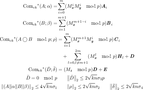
  and the proof-of-knowledge is accepting.

Sizes of Standard Deviations

$$\begin{aligned} \sigma _1 = 48\sqrt{ {k}{n}} {k}{m}{p}^2 ,&\sigma _2 = 72\sqrt{2 {k}{n}} {k}{m}{p}, \\ \sigma _3 = 24\sqrt{2 {k}{n}} {k}p (1+6 {k}{m}{p}) ,&\sigma _4 = 24\sqrt{2}{k}^2 {p}{n}\sigma _2 \end{aligned}$$

Security Analysis

Theorem 3

Given the statistically hiding, computationally binding commitment scheme based on SIS, the argument for multiplication triples has statistical completeness, statistical special honest verifier zero-knowledge and computational knowledge-soundness.

The proof of Theorem 3 can be found in the full version of this paper.

Efficiency. The above argument uses 7 moves of interaction and results in an overall 9 move argument when combined with the proof-of-knowledge sub-protocols. For the product argument, the prover must send $8{m}{k}+6{k}$ commitments to the verifier, and $14 {n}{k}$ integers as commitments openings, plus the communication for the proof-of-knowledge. Sub-linear communication is achieved by setting parameters as in Table 2. This gives communication of approximately $O(\sqrt{{N}\log {N}})$ elements of ${\mathbb {Z}}_{q}$.

For ${q}= \text {poly}({\lambda })$, the prover’s computational costs are given by $O({N}\log N (\log {\lambda })^2)$ bit operations for the prover. The verifier’s computational costs are dominated by computing the same types of linear combinations as the prover, giving computational costs of $O({N}( \log {\lambda })^3)$ bit operations.

7 Linear Constraint Argument Description

Using similar ideas to those in the multiplication protocol, in the full version of this paper, we give a protocol which allows the prover to prove that $N = {n}{m}{k}$ committed values satisfy the linear consistency relations

$$\begin{aligned} \sum _{i=1,j=1}^{{m},{k}} {\varvec{a}}_{i,j} \cdot {\varvec{w}}_{{u},{a,i,j}}+\sum _{i=1,j=1}^{{m},{k}} {\varvec{b}}_{i,j} \cdot {\varvec{w}}_{{u},{b,i,j}}+\sum _{i=1,j=1}^{{m},{k}} {\varvec{c}}_{i,j} \cdot {\varvec{w}}_{{u},{c,i,j}}=K_{{u}} \quad \text { for } {u}\in \{1,\ldots ,{U}\} \end{aligned}$$

(9)

Without loss of generality, we pad the linear consistency relations so that ${U}$ is divisible by ${k}$.

The protocol, security proof, and complexity analysis are very similar to that of the argument for proving multiplication triples in the previous section.

We select parameters for our protocol in Sect. 5.

Security Analysis

Theorem 4

Given the statistically hiding, computationally binding commitment scheme based in SIS, the argument for linear consistency constraints has statistical completeness, statistical special honest verifier zero-knowledge and computational knowledge-soundness.

The proof of Theorem 4 can be found in the full version of this paper.

Efficiency. The above argument uses 7 moves of interaction and results in an overall 9 move argument when combined with the proof-of-knowledge sub-protocols. For the product argument, the prover must send $7{k}{m}+9{k}-1$ commitments to the verifier, and $10{n}{k}+2{k}$ integers as commitment openings, plus the communication for the proof-of-knowledge. The asymptotic costs of the protocol are the same as for the argument for multiplication triples in the previous section. Combined with the proof of knowledge, this gives an arithmetic circuit argument with the stated efficiency.

8 Arithmetic Circuit Argument

The product protocol given in Sect. 6 and the linear consistency protocol given in Sect. 7 imply an arithmetic circuit protocol with the same asymptotic efficiency as the two subprotocols, in which the prover forms $O({m}{k})$ commitments, each to ${n}$ wire values in ${p}$, and runs both subprotocols in order to prove that they satisfy the arithmetic circuit, reusing the same commitments ${\varvec{A}}_i, {\varvec{B}}_i, {\varvec{C}}_i$ to the wires in both subprotocols.

This yields a zero-knowledge argument for arithmetic circuit satisfiability with communication costs $O(\sqrt{{N}\log {N}})$ elements of ${\mathbb {Z}}_{q}$, computational costs of $O({N}\log {N})$ for the prover, and approximately $O({N})$ for the verifier.

References

Ames, S., Hazay, C., Ishai, Y., Venkitasubramaniam, M.: Ligero: lightweight sublinear arguments without a trusted setup. In: Thuraisingham et al. [TEMX17], pp. 2087–2104
Ajtai, M.: Generating hard instances of lattice problems (extended abstract). In: 28th ACM STOC, pp. 99–108. ACM Press, May 1996
Banaszczyk, W.: New bounds in some transference theorems in the geometry of numbers. Mathematische Annalen 296, 625–635 (1993)
Bunz, B., Bootle, J., Boneh, D., Poelstra, A., Maxwell, G.: Bulletproofs: short proofs for confidential transactions and more. Cryptology ePrint Archive, Report 2017/1066 (2017). https://eprint.iacr.org/2017/1066
Bootle, J., Cerulli, A., Chaidos, P., Groth, J., Petit, C.: Efficient zero-knowledge arguments for arithmetic circuits in the discrete log setting. In: Fischlin and Coron [FC16], pp. 327–357
Bitansky, N., Canetti, R., Chiesa, A., Tromer, E.: From extractable collision resistance to succinct non-interactive arguments of knowledge, and back again. In: Goldwasser, S. (ed.) ITCS 2012, pp. 326–349. ACM, January 2012
Bitansky, N., Canetti, R., Chiesa, A., Tromer, E.: Recursive composition and bootstrapping for SNARKS and proof-carrying data. In: Boneh, D., Roughgarden, T., Feigenbaum, J. (eds.) 45th ACM STOC, pp. 111–120. ACM Press, June 2013
Bootle, J., Cerulli, A., Ghadafi, E., Groth, J., Hajiabadi, M., Jakobsen, S.K.: Linear-time zero-knowledge proofs for arithmetic circuit satisfiability. In: Takagi, T., Peyrin, T. (eds.) ASIACRYPT 2017, Part III. LNCS, vol. 10626, pp. 336–365. Springer, Cham (2017). https://doi.org/10.1007/978-3-319-70700-6_12
Benhamouda, F., Camenisch, J., Krenn, S., Lyubashevsky, V., Neven, G.: Better zero-knowledge proofs for lattice encryption and their application to group signatures. In: Sarkar, P., Iwata, T. (eds.) ASIACRYPT 2014, Part I. LNCS, vol. 8873, pp. 551–572. Springer, Heidelberg (2014). https://doi.org/10.1007/978-3-662-45611-8_29
Bendlin, R., Damgård, I.: Threshold decryption and zero-knowledge proofs for lattice-based cryptosystems. In: Micciancio, D. (ed.) TCC 2010. LNCS, vol. 5978, pp. 201–218. Springer, Heidelberg (2010). https://doi.org/10.1007/978-3-642-11799-2_13
Baum, C., Damgård, I., Larsen, K.G., Nielsen, M.: How to prove knowledge of small secrets. In: Robshaw, M., Katz, J. (eds.) CRYPTO 2016, Part III. LNCS, vol. 9816, pp. 478–498. Springer, Heidelberg (2016). https://doi.org/10.1007/978-3-662-53015-3_17
Baum, C., Damgård, I., Oechsner, S., Peikert, C.: Efficient commitments and zero-knowledge protocols from ring-SIS with applications to lattice-based threshold cryptosystems. Cryptology ePrint Archive, Report 2016/997 (2016). http://eprint.iacr.org/2016/997
Bai, S., Galbraith, S.D.: An improved compression technique for signatures based on learning with errors. In: Benaloh, J. (ed.) CT-RSA 2014. LNCS, vol. 8366, pp. 28–47. Springer, Cham (2014). https://doi.org/10.1007/978-3-319-04852-9_2
Benhamouda, F., Krenn, S., Lyubashevsky, V., Pietrzak, K.: Efficient zero-knowledge proofs for commitments from learning with errors over rings. In: Pernul, G., Ryan, P.Y.A., Weippl, E. (eds.) ESORICS 2015, Part I. LNCS, vol. 9326, pp. 305–325. Springer, Cham (2015). https://doi.org/10.1007/978-3-319-24174-6_16
Cramer, R., Damgård, I.: Linear zero-knowledge - a note on efficient zero-knowledge proofs and arguments. In: 29th ACM STOC, pp. 436–445. ACM Press, May 1997
Chase, M., Derler, D., Goldfeder, S., Orlandi, C., Ramacher, S., Rechberger, C., Slamanig, D., Zaverucha, G.: Post-quantum zero-knowledge and signatures from symmetric-key primitives. In: Thuraisingham et al. [TEMX17], pp. 1825–1842
Cramer, R., Damgård, I., Keller, M.: On the amortized complexity of zero-knowledge protocols. J. Cryptol. 27(2), 284–316 (2014)
Cramer, R., Damgård, I., Xing, C., Yuan, C.: Amortized complexity of zero-knowledge proofs revisited: achieving linear soundness slack. In: Coron and Nielsen [CN17], pp. 479–500
Coron, J.-S., Nielsen, J.B. (eds.): EUROCRYPT 2017, Part I. LNCS, vol. 10210. Springer, Cham (2017). https://doi.org/10.1007/978-3-319-56620-7
Damgård, I.: On \(\Sigma \)-protocols (2010). http://www.cs.au.dk/~ivan/Sigma.pdf
Ducas, L., Durmus, A., Lepoint, T., Lyubashevsky, V.: Lattice signatures and bimodal gaussians. In: Canetti, R., Garay, J.A. (eds.) CRYPTO 2013, Part I. LNCS, vol. 8042, pp. 40–56. Springer, Heidelberg (2013). https://doi.org/10.1007/978-3-642-40041-4_3
Damgård, I., López-Alt, A.: Zero-knowledge proofs with low amortized communication from lattice assumptions. In: Visconti, I., De Prisco, R. (eds.) SCN 2012. LNCS, vol. 7485, pp. 38–56. Springer, Heidelberg (2012). https://doi.org/10.1007/978-3-642-32928-9_3
del Pino, R., Lyubashevsky, V.: Amortization with fewer equations for proving knowledge of small secrets. In: Katz, J., Shacham, H. (eds.) CRYPTO 2017, Part III. LNCS, vol. 10403, pp. 365–394. Springer, Cham (2017). https://doi.org/10.1007/978-3-319-63697-9_13
Fischlin, M., Coron, J.-S. (eds.): EUROCRYPT 2016, Part II. LNCS, vol. 9666. Springer, Heidelberg (2016). https://doi.org/10.1007/978-3-662-49896-5
Goldreich, O., Goldwasser, S.: On the limits of non-approximability of lattice problems. In: 30th ACM STOC, pp. 1–9. ACM Press, May 1998
Gentry, C., Groth, J., Ishai, Y., Peikert, C., Sahai, A., Smith, A.D.: Using fully homomorphic hybrid encryption to minimize non-interative zero-knowledge proofs. J. Cryptol. 28(4), 820–843 (2015)
Gennaro, R., Gentry, C., Parno, B., Raykova, M.: Quadratic span programs and succinct NIZKs without PCPs. In: Johansson, T., Nguyen, P.Q. (eds.) EUROCRYPT 2013. LNCS, vol. 7881, pp. 626–645. Springer, Heidelberg (2013). https://doi.org/10.1007/978-3-642-38348-9_37
Goldreich, O., Håstad, J.: On the complexity of interactive proofs with bounded communication. Inf. Process. Lett. 67, 205–214 (1998)
Güneysu, T., Lyubashevsky, V., Pöppelmann, T.: Practical lattice-based cryptography: a signature scheme for embedded systems. In: Prouff, E., Schaumont, P. (eds.) CHES 2012. LNCS, vol. 7428, pp. 530–547. Springer, Heidelberg (2012). https://doi.org/10.1007/978-3-642-33027-8_31
Giacomelli, I., Madsen, J., Orlandi, C.: Zkboo: faster zero-knowledge for boolean circuits. In: 25th USENIX Security Symposium, pp. 1069–1083 (2016)
Goldwasser, S., Micali, S., Rackoff, C.: The knowledge complexity of interactive proof-systems (extended abstract). In: 17th ACM STOC, pp. 291–304. ACM Press, May 1985
Gama, N., Nguyen, P.Q.: Predicting lattice reduction. In: Smart, N. (ed.) EUROCRYPT 2008. LNCS, vol. 4965, pp. 31–51. Springer, Heidelberg (2008). https://doi.org/10.1007/978-3-540-78967-3_3
Guillou, L.C., Quisquater, J.-J.: A practical zero-knowledge protocol fitted to security microprocessor minimizing both transmission and memory. In: Barstow, D., et al. (eds.) EUROCRYPT 1988. LNCS, vol. 330, pp. 123–128. Springer, Heidelberg (1988). https://doi.org/10.1007/3-540-45961-8_11
Groth, J.: Linear algebra with sub-linear zero-knowledge arguments. In: Halevi, S. (ed.) CRYPTO 2009. LNCS, vol. 5677, pp. 192–208. Springer, Heidelberg (2009). https://doi.org/10.1007/978-3-642-03356-8_12
Groth, J.: Short pairing-based non-interactive zero-knowledge arguments. In: Abe, M. (ed.) ASIACRYPT 2010. LNCS, vol. 6477, pp. 321–340. Springer, Heidelberg (2010). https://doi.org/10.1007/978-3-642-17373-8_19
Groth, J.: A verifiable secret shuffle of homomorphic encryptions. J. Cryptol. 23(4), 546–579 (2010)
Groth, J.: On the size of pairing-based non-interactive arguments. In: Fischlin and Coron [FC16], pp. 305–326
Goldreich, O., Vadhan, S.P., Wigderson, A.: On interactive proofs with a laconic prover. Comput. Complex. 11(1–2), 1–53 (2002)
Gentry, C., Wichs, D.: Separating succinct non-interactive arguments from all falsifiable assumptions. In: Fortnow, L., Vadhan, S.P. (eds.) 43rd ACM STOC, pp. 99–108. ACM Press, June 2011
Ishai, Y., Kushilevitz, E., Ostrovsky, R., Sahai, A.: Zero-knowledge from secure multiparty computation. In: Johnson, D.S., Feige, U. (eds.) 39th ACM STOC, pp. 21–30. ACM Press, June 2007
Kilian, J.: A note on efficient zero-knowledge proofs and arguments (extended abstract). In: 24th ACM STOC, pp. 723–732. ACM Press, May 1992
Kalai, Y.T., Raz, R.: Interactive PCP. In: Aceto, L., Damgård, I., Goldberg, L.A., Halldórsson, M.M., Ingólfsdóttir, A., Walukiewicz, I. (eds.) ICALP 2008, Part II. LNCS, vol. 5126, pp. 536–547. Springer, Heidelberg (2008). https://doi.org/10.1007/978-3-540-70583-3_44
Lipmaa, H.: Progression-free sets and sublinear pairing-based non-interactive zero-knowledge arguments. In: Cramer, R. (ed.) TCC 2012. LNCS, vol. 7194, pp. 169–189. Springer, Heidelberg (2012). https://doi.org/10.1007/978-3-642-28914-9_10
Lyubashevsky, V., Micciancio, D.: Generalized compact knapsacks are collision resistant. In: Bugliesi, M., Preneel, B., Sassone, V., Wegener, I. (eds.) ICALP 2006, Part II. LNCS, vol. 4052, pp. 144–155. Springer, Heidelberg (2006). https://doi.org/10.1007/11787006_13
Lyubashevsky, V., Neven, G.: One-shot verifiable encryption from lattices. In: Coron and Nielsen [CN17], pp. 293–323
Ling, S., Nguyen, K., Stehlé, D., Wang, H.: Improved zero-knowledge proofs of knowledge for the ISIS problem, and applications. In: Kurosawa, K., Hanaoka, G. (eds.) PKC 2013. LNCS, vol. 7778, pp. 107–124. Springer, Heidelberg (2013). https://doi.org/10.1007/978-3-642-36362-7_8
Lyubashevsky, V.: Fiat-Shamir with aborts: applications to lattice and factoring-based signatures. In: Matsui, M. (ed.) ASIACRYPT 2009. LNCS, vol. 5912, pp. 598–616. Springer, Heidelberg (2009). https://doi.org/10.1007/978-3-642-10366-7_35
Lyubashevsky, V.: Lattice signatures without trapdoors. In: Pointcheval, D., Johansson, T. (eds.) EUROCRYPT 2012. LNCS, vol. 7237, pp. 738–755. Springer, Heidelberg (2012). https://doi.org/10.1007/978-3-642-29011-4_43
Micciancio, D., Regev, O.: Worst-case to average-case reductions based on Gaussian measures. In: 45th FOCS, pp. 372–381. IEEE Computer Society Press, October 2004
Micciancio D., Regev O.: Lattice-based Cryptography. In: Bernstein, D.J., Buchmann, J., Dahmen, E. (eds.) Post-Quantum Cryptography. Springer, Heidelberg (2009). https://doi.org/10.1007/978-3-540-88702-7_5
Micciancio, D., Vadhan, S.P.: Statistical zero-knowledge proofs with efficient provers: lattice problems and more. In: Boneh, D. (ed.) CRYPTO 2003. LNCS, vol. 2729, pp. 282–298. Springer, Heidelberg (2003). https://doi.org/10.1007/978-3-540-45146-4_17
Parno, B., Howell, J., Gentry, C., Raykova, M.: Pinocchio: nearly practical verifiable computation. In: 2013 IEEE Symposium on Security and Privacy, pp. 238–252. IEEE Computer Society Press, May 2013
Peikert, C., Rosen, A.: Efficient collision-resistant hashing from worst-case assumptions on cyclic lattices. In: Halevi, S., Rabin, T. (eds.) TCC 2006. LNCS, vol. 3876, pp. 145–166. Springer, Heidelberg (2006). https://doi.org/10.1007/11681878_8
Regev, O.: On lattices, learning with errors, random linear codes, and cryptography. In: Gabow, H.N., Fagin, R. (eds.) 37th ACM STOC, pp. 84–93. ACM Press, May 2005
Schnorr, C.-P.: Efficient signature generation by smart cards. J. Cryptol. 4(3), 161–174 (1991)
Stern, J.: A new identification scheme based on syndrome decoding. In: Stinson, D.R. (ed.) CRYPTO 1993. LNCS, vol. 773, pp. 13–21. Springer, Heidelberg (1994). https://doi.org/10.1007/3-540-48329-2_2
Thuraisingham, B.M., Evans, D., Malkin, T., Xu, D. (eds.): ACM CCS 17. ACM Press, October/November (2017)
Author information
Authors and Affiliations
Corresponding author
Editor information
Editors and Affiliations
Rights and permissions
Copyright information
© 2018 International Association for Cryptologic Research
About this paper
Cite this paper
Baum, C., Bootle, J., Cerulli, A., del Pino, R., Groth, J., Lyubashevsky, V. (2018). Sub-linear Lattice-Based Zero-Knowledge Arguments for Arithmetic Circuits. In: Shacham, H., Boldyreva, A. (eds) Advances in Cryptology – CRYPTO 2018. CRYPTO 2018. Lecture Notes in Computer Science(), vol 10992. Springer, Cham. https://doi.org/10.1007/978-3-319-96881-0_23
Download citation
DOI: https://doi.org/10.1007/978-3-319-96881-0_23
Published:
Publisher Name: Springer, Cham
Print ISBN: 978-3-319-96880-3
Online ISBN: 978-3-319-96881-0
eBook Packages: Computer ScienceComputer Science (R0)