Analytical Method to Study the Ultimate Bearing Capacity of Containment for Floating Nuclear Power Plants Considering Wave Loads

Abstract

In floating nuclear power plant (FNPP), important equipment such as nuclear pressure vessel, pressure pipeline and pressurizer are installed in the containment, which is the last safety barrier of the reactor primary circuit of FNPP. The ultimate bearing capacity of containment is one of the important safety indexes of FNPP. In this study, considering the wave load, internal pressure load and their corresponding combination conditions in the sea area of FNPP, the overall finite element model of FNPP and the local finite element model of containment are established by using ANSYS software. The ultimate bearing capacity of containment structure is analyzed by nonlinear method. The ultimate internal pressure that the containment can bear is analyzed based on the wave load. Two methods are used to analyze the ultimate internal pressure that the containment can withstand. One is direct analysis method to directly carry out nonlinear analysis of the whole ship model. The other, called indirect analysis method, first makes a linear analysis of the whole ship model to calculate the input load transmitted from the marine environment to the containment through the containment support, and then uses the nonlinear method to analyze the ultimate internal pressure that the containment can withstand. The analysis results of the above two methods show that the ultimate bearing capacity of the containment is basically consistent, while the efficiency of the indirect analysis method is higher. In addition, the ultimate bearing capacity of the containment is far beyond the design requirements considering the wave load.

1 Introduction

At present, the research on the ultimate strength of offshore platform structures has become a hot topic in the field of international offshore engineering. For the structural design of offshore platforms, the limit state based design method has been introduced [1]. Through the calculation of the ultimate strength of the platform, the dangerous component parts can be predicted, and the local strengthening of the components can timely control the degree of damage and reduce the potential crisis. Up to now, scholars have put forward different research methods for the ultimate strength of ship structures, and several of them have been widely recognized and gradually improved. At present, the ultimate strength analysis methods of hull structures mainly include: direct calculation method, nonlinear finite element method, progressive collapse method, ideal structural element method and model test method.

The direct calculation method is also called Caldwell method. In 1965, Caldwell [2] first proposed the plastic behavior of the total longitudinal strength of surface ships, and derived the analytical formula of the total longitudinal ultimate strength. In view of the limitations of Caldwell method, Smith [3] proposed a relatively simple method based on Caldwell method, taking into account the reduction of strength after the member reaches the ultimate strength, and thus the progressive collapse method is also called Smith method. Another simple method for progressive failure analysis of hull beams is the ideal structural element method (ISUM) proposed by Japanese scholar Ueda et al. [4] in the 1980s. With the general improvement of computer hardware level, the finite element method (FEM) has been applied more often to engineering problems. Compared with the above analysis methods, the physical test can more directly reflect the collapse process of the ship structure and measure the ultimate strength of the structure. Dow [5] established a hull beam model of a frigate at a scale of 1/3 and conducted ultimate strength tests. Nishihara [6] conducted a series of collapse tests under pure bending load on a box beam model similar to the corresponding ship structure. The phenomena and results observed in the experiment also have high reference value for theoretical calculation and numerical simulation.

2 Nonlinear Analysis Method

Chen [7] et al. proposed a finite element method for hull ultimate bearing analysis, which is applicable to any loading type and structural model. This method introduces three element types: beam element, plate element and orthotropic plate element, which can analyze the limit state of the structure under static or dynamic loads, and It can also analyze the overall response of a single member (deck, side, bulkhead, longitudinal girder, etc.) and consider the response of the hull under the combined action of bending moment, torque and shear force. Kutt [8] et al. used nonlinear analysis method to analyze the longitudinal ultimate strength of four hulls, reflecting the interaction between various local and overall failure modes and the interaction between the elastic−plastic, buckling and post buckling effects of materials.

With the development of calculation technology and nonlinear finite element, many large general finite element programs, such as NASTRAN, ANSYS, ABAQUS, Marc, have been applied to the ultimate strength calculation of ship structures. Based on the nonlinear finite element method, this chapter will use the finite element software ANSYS to study the solution method.

2.1 Arc length method

The arc length method is a static analysis method based on the Newton Raphson iterative solution of the nonlinear static equilibrium equation of the structure [9]. Its basic idea is to set a parameter (arc length $l$) to control the incremental iteration and convergence of the equilibrium equation.

$$ \{ P\} - \{ I\} = 0 $$

(1)

$$ [K_{T} ]\{ \Delta u\} = \{ \Delta P\} - \{ R\} $$

(2)

where $[K_{T} ]$ is tangent stiffness matrix, $\{ \Delta u\}$ is the displacement increment, $\{ \Delta P\}$ is load increment, $\{ R\}$ is residual force.

When using the arc length method, let the $i - 1$ load step converge to $(x_{i - 1} ,P_{i - 1} )$ , for the $i$ load step, $j$ iterations are required to reach the new convergence point $(x_{i} ,P_{i} )$. Step $i$ iterates the true load size $\{ \Delta P\}$ acting on the structure, which is determined by the load increment factor $\Delta \lambda_{i}$ and the input external load $\{ P_{ref} \}$,

$$ \{ \Delta P\}_{i} = \Delta \lambda_{i} \{ P_{ref} \} $$

(3)

By introducing Eq. (3) into Eq. (2), the incremental form of iteration i of arc length method can be obtained:

$$ [K_{T} ]\{ \Delta u\}_{i} = \Delta \lambda_{i} \{ P_{ref} \} - \{ R\}_{i} $$

(4)

The position of the equilibrium point in step $i$ is obtained by Newton Raphson iteration with the equilibrium point calculated in step $i - 1$ as the center of the circle and the arc length increment $\Delta i$ as the radius, as shown in Fig. 1. The arc length increment $\Delta l_{i}$, load increment factor $\Delta \lambda_{i}$ and displacement increment $\left\{ {\Delta u} \right\}_{i}$ of each step satisfy the governing equation of Eq. (5).

$$ \Delta l_{i}^{2} = \left| {\left\{ {\Delta u} \right\}_{i} } \right|^{2} + \left| {\Delta \lambda_{i} \left\{ {P\,_{ref} } \right\}} \right|^{2} $$

(5)

Fig. 1.

Load displacement curve

Through iteration, until the residual force is within the tolerance {R}, when the iteration of step $i$ is completed, there are:

$$ {\text{Load }}\,{\text{array}}\,\{ P\} i = \sum\nolimits_{i} {\{ \Delta P\} }_{i} = \sum\nolimits_{i} {\Delta \lambda_{i} \{ P_{ref} \} } $$

(6)

$$ {\text{Displacement }}\,{\text{array}}\,\{ u\}_{i} = \sum\nolimits_{i} {\{ \Delta u\} }_{i} $$

(7)

$$ {\text{arc}}\,{\text{ length}}\,l_{i} = \sum\nolimits_{i} {\Delta l_{i} } $$

(8)

The arc length increment $\Delta l$ contains the information of load increment and displacement increment at the same time. As long as the appropriate iteration step is selected, the arc length method can track the load displacement equilibrium path of the structure in the process of loading and unloading, and effectively solve the ‘step’ problem in the limit equilibrium path.

2.2 Quasi Static Method

In essence, the quasi−static analysis method is a dynamic solution process of structure. The basic idea of the quasi−static method is to simulate the static problems with the dynamic analysis of slow loading, which is based on the explicit solution of the structural nonlinear motion equation (central difference method).

The central difference method is used to perform explicit time integration for the structural nonlinear motion Eq. (9). The dynamic conditions of the next incremental step are calculated from the dynamic conditions of the previous incremental step until the end of the solution time.

$$ [M]\{ \ddot{u}\} = \{ P\} - \{ I\} $$

(9)

where $\{ P\} - \{ I\}$ is the mass matrix, $\{ \ddot{u}\}$ is the acceleration array, $\{ P\}$ is the load array, and $\{ I\}$ is the internal force array.

The key to the solution of quasi−static method is to set a reasonable loading rate. Too fast loading rate leads to severe local deformation of the solution results, which makes the calculation results deviate from the requirements of “quasi−static”, and the load displacement curve oscillates. However, too slow loading rate increases the calculation time greatly, which means a long loading time. Therefore, we usually take several different loading rates for comparison and analysis, and then select the appropriate loading rate when analyzing.

By studying the various energies in the model, we can evaluate whether the simulation produces the correct quasi−static response.

$$ E_{KE} + E_{FD} + E_{I} + E_{V} - E_{W} = E_{total} $$

(10)

where $E_{KE}$ is the structural kinetic energy, $E_{FD}$ is the energy dissipated and absorbed by friction, $E_{I}$ is the internal energy, including plastic and elastic strain energy, $E_{V}$ is the energy dissipated and absorbed by viscosity, $E_{W}$ is the work done by external forces, and $E_{total}$ is the total energy in the system, which is a constant.

If the finite element simulation is quasi−static, the internal energy of the system is almost equal to the work done by the external force. Generally, the viscous dissipation energy is very small, unless material damping, viscoelastic materials or discrete shock absorbers are used. Therefore, we can determine that the inertia force is ignored according to the small flow velocity of the material in the model in the quasi−static process. It can be inferred from these two conditions that the kinetic energy is also very small. In most processes, the ratio of kinetic energy to strain energy of the structural model is an important criterion to judge whether the loading rate is appropriate. As a general rule, the general quasi−static requirement is that the ratio of kinetic energy to strain energy is less than 5%.

The applied loads are required to be as smooth as possible for accurate and efficient quasi−static problems. Stress waves arise from sudden, rapid movements that will cause oscillations or inaccurate results. The loading method shall be as smooth as possible, and the acceleration between two incremental steps shall only change by a small amount. If the acceleration is smooth, the varying velocity and displacement are smooth.

Since the central difference method is a conditionally stable algorithm, the time step $\Delta t$ must be less than the stability limit $\Delta t_{stable}$ to ensure the stability of the solution:

$$ \Delta t_{stable} = 2/\omega_{\max } \ge \Delta t^{e} $$

(11)

where $\omega_{\max }$ is the highest natural frequency of the structure, $\Delta t^{e}$ is the stable time step of the element with the smallest size in the structural model, $\Delta t^{e}$ is related to the characteristic scale $L^{e}$, elastic modulus $E$ and material density of the element $\rho$ Is the upper bound of the stability limit $\Delta t_{stable}$:

$$ \Delta t^{e} = L^{e} /\sqrt {E/P} $$

(12)

In the calculation, since the highest order frequency $\omega_{\max }$ of the structure is not easy to obtain, the time step $\Delta t$ is taken as $\Delta t^{e}$.

Compared with the arc length method, the quasi−static method has no convergence problem because the central difference method is used for explicit integration, and can solve more complex structural collapse problems such as material failure and structural self−contact. Because the time step $\Delta t$ is often small, the quasi−static loading is slow and the solution time is very long when solving the limit state problem, which can be adjusted by means of mass amplification.

3 Calculation of Ultimate Bearing Capacity Under Different Working Conditions

According to the classification of marine environmental conditions and the guide for buckling strength assessment of offshore engineering structures, the load distribution characteristics of the hull under different marine conditions are calculated respectively. The finite element model of the floating nuclear power plant is established based on ANSYS software, and then the load borne by the hull is applied to the finite element analysis model of the floating nuclear power plant to calculate and analyze the stress and displacement response of the overall structure of the floating nuclear power plant and the steel containment, and carry out the calculation of the ultimate bearing capacity of the containment of the floating nuclear power plant under different working conditions.

The finite element model of the hull structure is constructed with shell181 and beam188 elements. The mesh size of the bottom and supporting parts of the containment is 0.1 M, the mesh size of the upper part of the containment is 0.2 m, and the mesh size of the rest is 0.8 m. The total number of elements on the whole ship is about 1.56 million (Figs. 2 and 3).

Fig. 2.

Overall finite element model of ship structure

Fig. 3.

Finite element model of containment

3.1 Calculation and Analysis of Ultimate Bearing Capacity Under Internal Pressure Condition of Containment

The internal pressure load is loaded inside the containment by uniformly distributing the load in the element, and the fixed support constraint is added at the bottom node of the compartment where the containment is located. Considering the influence of material hardening on the ultimate strength of the structure, the material constitutive relationship is set as shown in the figure below (Fig. 4).

Fig. 4.

Constitutive relation of material model

Sort out the calculation results, and select the top with the largest deformation and change rate as the analysis point. The load displacement curve is shown in the figure below (Fig. 5).

Fig. 5.

Load displacement relationship of steel containment top node

The analysis shows that when the internal pressure load is below 2 MPa, the slope of the curve does not change, showing a linear growth trend, indicating that the structure is still in the elastic deformation order, and the equivalent plastic strain is 0; When the internal pressure load increases from 2 MPa, the curvature in the load displacement curve begins to change, indicating that the structure begins to enter the plastic deformation stage.

• (1) Double limit method

  The double elastic slope method is used to determine the limit load in ASME VIII−2. In this method, the origin of load displacement curve is taken as the starting point to draw the straight line of elastic slope in the elastic stage, and then another straight line is drawn to meet the elastic slope whose slope is equal to twice. The load value projected on the vertical coordinate by the intersection of the straight line and the load displacement curve is the limit load value [10] (Fig. 6).

  Fig. 6.

  

  Load displacement relation of double limit method

It can be seen from the figure that the limit load value determined by this model based on the more accurate load displacement curve after reducing the load increment step and using the double elastic slope method is about 3.442 MPa. This method is an artificial regulation and is greatly affected by human factors. The determined limit load value may have great dispersion and error.

• (2) Double tangent intersection method

  The double tangent intersection method is the method for determining the limit load in the European standard EN 13445. Based on the load displacement curve, the tangent lines of elastic stage and plastic stage are drawn respectively. The tangent of the plastic section adopts the first−order fitting function obtained from the plastic section data processed by the least square method, and the load value projected on the longitudinal coordinate by the intersection of the two tangents is the limit load value [11] (Fig. 7).

  Fig. 7.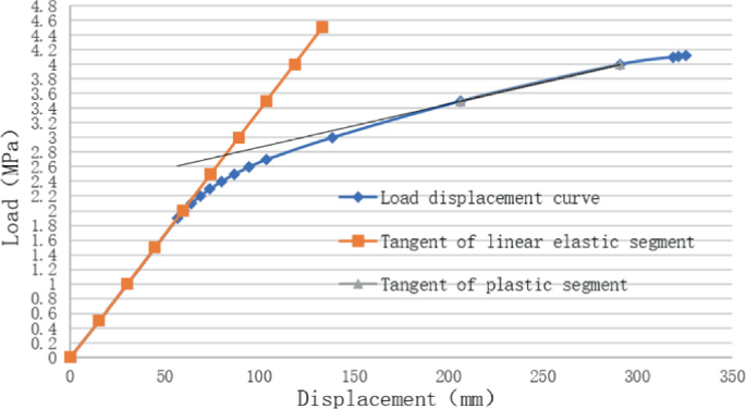

  

  Load displacement relationship of double tangent intersection method

It can be seen from the figure that the limit load value determined by the model based on the load displacement curve and the double tangent intersection method is about 2.755 MPa, which is completely determined by the curve itself, and is less affected by human factors than the double elastic slope method.

3.2 Calculation and Analysis of Ultimate Bearing Capacity of Containment Vessel Under Combined Wave Load and Internal Pressure

Taking the 100 year return period sea conditions, set the wave height as 9 m, calculate the loading of the finite element model of the whole ship of the floating nuclear power plant, and analyze the waves in 13 directions. Set a wave direction every 15° from 0° to 180°. The schematic diagram of wave incidence angle is shown in the following figure (Fig. 8):

Fig. 8.

Schematic diagram of wave incidence angle

In order to improve the calculation efficiency, the displacement structure response in the overall finite element model under wave load is calculated, and then the node displacement of the containment support in the overall model is extracted and loaded at the corresponding node of the containment finite element model as a boundary condition. Take the nodes with the stress value greater than 50 MPa in the containment, and compare the stress value of the containment nodes in the finite element model of the whole ship with the corresponding node stress value on the separate containment model. Some results are shown in the table below (Table 1).

Table 1. Comparison of node stress (zero degree wave load as an example)

It is known from the data that the acceleration has little effect on the node stress, and the node stress on the containment mainly comes from the deformation of the structure. In order to simulate the structural response under the wave load in the separate containment model, compare the stress values of the corresponding nodes in the whole ship model and the separate containment model, and load twice the displacement structural response of the containment support node to the corresponding node of the separate containment, As the initial displacement boundary condition, the ultimate bearing capacity of wave load under the combined action of internal pressure is analyzed. The internal pressure loading method is the same as above.

The double limit method is used to analyze the ultimate bearing capacity of the structure as follows (Fig. 9).

Fig. 9.

Load displacement relation of double limit method

It can be seen from the figure that the limit load value determined by the model based on the more accurate load displacement curve after reducing the load increment step and using the double elastic slope method is about 3.45 MPa.

The ultimate bearing capacity of the structure is analyzed by the double tangent intersection method as follows (Fig. 10).

Fig. 10.

Load displacement relationship of double tangent intersection method

It can be seen from the figure that the limit load value determined by the model based on the load displacement curve and the double tangent intersection method is about 2.56 MPa.

According to the constitutive characteristics of the material, when the stress of the material exceeds the tensile strength of 585 mpa, it is considered that the strength failure of the material occurs there. According to the finite element analysis, when the internal pressure of the structure is 3.1 Mpa, the maximum value of the maximum stress point is 584 mpa. Therefore, it is considered that the structure has strength failure at 3.1 Mpa (the stress nephogram is shown in the figure below) (Fig. 11).

Fig. 11.

Stress nephogram of steel containment in case of strength failure

4 Conclusions

Based on an engineering example model, this paper studies the analysis method of the ultimate bearing capacity of the containment of a floating nuclear power plant, and draws the following conclusions.

• 1. Based on the finite element analysis software, the stress−strain nephogram and load displacement curve are accurately calculated, and the limit load can be judged and determined by the double elastic slope method and the double tangent intersection method. In terms of the accuracy of determining the limit load value, the double tangent intersection method is within an acceptable range due to the difficult determination of the tangent in the plastic stage, and the double elastic slope method is susceptible to human factors, so the accuracy is conservative.

• 2. Considering the wave load, compared with the finite element nonlinear analysis of the whole ship model, the method of extracting the load at the containment support in the overall model for linear calculation and loading it on the corresponding node of the local model of the containment is adopted to ensure the accurate load loading, shorten the calculation time and improve the calculation efficiency.

• 3. In the method of indirect loading, the impact of wave load on the containment of floating nuclear power plant is divided into two parts: the impact of structural deformation and the impact of structural acceleration. Compared with the impact of structural deformation on the ultimate bearing capacity of the containment, the impact of structural acceleration is relatively small and can be ignored.

References

Veritas, D.N.: Design of Offshore Steel Structures - General (lrfd Method) (2004)
Caldwell, J.B.: Ultimate longitudinal strengt. trans rina (1965)
Smith, C.S.: Influence of local compressive failure on ultimate longitudinal strength of a ship's hul. In: Proceedings of International Symposium on Practical Design in Shipbuilding, Tokyo, Japan (1977)
Ueda, Y., Rashed, S.M.H., Paik, J.K.: Plate and stiffened plate units of the idealized structural unit method (1st Report) under in plane loading. J. Soc. Naval Arch. Jpn. (1984)
Dow, R.S.: Testing and analysis of 1/3-scale welded steel frigate model. In : Proceedings of the International Conference on Advances in Marine Structures, pp. 749–773 (1991)
Nishihara, S., Engineering, O.: Ultimate longitudinal strength of mid-ship cross section. Naval Arch. 22, 200–214 (1984)
Chen, Y.K., Kutt, L.M., Piaszezyk, C.M., et al.: Ultimate strength of ship structures. Trans. SNAME, pp. 149–168 (1983)
Kutt, L.M., Piaszczyk, C.M., Yung-Kuang, C., et al.: Evaluation of the longitudinal ultimate strength of various ship hull configurations. Trans.-Soc. Naval Arch. Marine Eng. 93, 33–53 (1985)
Peng, D., Zhang, S.: Study on three finite element methods for structural ultimate strength analysis. China Offshore Platform 2, 5 (2010)
Li, J.: Mechanical basis of pressure vessel design and its standard application (2004)
Spraragen, W.: Unfired pressure vessels. Indengchem 23(2), 220–226 (1931)
Author information
Authors and Affiliations
Corresponding author
Editor information
Editors and Affiliations
Rights and permissions
Open Access This chapter is licensed under the terms of the Creative Commons Attribution 4.0 International License (http://creativecommons.org/licenses/by/4.0/), which permits use, sharing, adaptation, distribution and reproduction in any medium or format, as long as you give appropriate credit to the original author(s) and the source, provide a link to the Creative Commons license and indicate if changes were made.
The images or other third party material in this chapter are included in the chapter's Creative Commons license, unless indicated otherwise in a credit line to the material. If material is not included in the chapter's Creative Commons license and your intended use is not permitted by statutory regulation or exceeds the permitted use, you will need to obtain permission directly from the copyright holder.
Copyright information
© 2023 The Author(s)
About this paper
Cite this paper
Mu, S., Li, L., Zhang, M., Liu, H., Qu, X. (2023). Analytical Method to Study the Ultimate Bearing Capacity of Containment for Floating Nuclear Power Plants Considering Wave Loads. In: Liu, C. (eds) Proceedings of the 23rd Pacific Basin Nuclear Conference, Volume 1. PBNC 2022. Springer Proceedings in Physics, vol 283. Springer, Singapore. https://doi.org/10.1007/978-981-99-1023-6_70
Download citation
DOI: https://doi.org/10.1007/978-981-99-1023-6_70
Published:
Publisher Name: Springer, Singapore
Print ISBN: 978-981-99-1022-9
Online ISBN: 978-981-99-1023-6
eBook Packages: Physics and AstronomyPhysics and Astronomy (R0)