Specify Boundary Conditions

Abstract

The governing equations of incompressible turbulent flow with the k-ε turbulence model can be expressed in the following general form:

Appendices

Practice-6: Simulation of Computer Rack in Data Center

Example Project: Simplified Rack Boundary Conditions for Data Center Models

Background:

Data centers are energy suckers due to high electricity demand for both intensive computing and cooling. The layout and design of a data center can make a significant difference in its energy use and the consequences of improper data center design can be dramatic. Cooling energy in poorly designed data centers can constitute up to 50% of its energy use. CFD plays an important role in aiding the layout design and management of data centers. While the use of CFD modeling is common in data center design, there are some important issues that need to be resolved.

Modeling the computer/server rack is one of the critical pieces in the design process. Often this is done as a black box rather than modeling the rack in detail. Modeling a computer rack as a black box has been carried out in numerous data center studies, but rarely has it been validated against experimental temperature and velocity data. In a black box model, room conditions are put into the front (inlet) of the rack and the added enthalpy outputs come from the back of the rack (outlet). One of the central issues with this approach is the question of which boundary conditions for the rack produce acceptable accuracy. The goal of this project was to develop a set of easily reproducible boundary conditions and validate them against sets of experimental data.

Simulation Details:

His study developed two distinct CFD models, an open box model (OBM) and a black box model (BBM). Both models were designed to be simple and require minimal user inputs. All models were developed using commercially available CFD software. The OBM was developed first and its purpose was to be an interim step to inform the development of the BBM. While it was very simplified in its detail, the OBM was still an approximation of the server simulator and allowed for air to flow through the rack model. The BBM, by contrast, was a solid box. It took inputs at the rack inlet and outputted modified values at the rack outlet. Its assumptions were tested both against the experimental data and the OBM. Both models shared the Boussinesq approximation and the κ-ε turbulence model used in the RANS equations. All surfaces were modeled as adiabatic surfaces and radiation models were not used.

• (1) Open Box Model (OBM)

Figure 6.4 shows the layout of the experiment setup and the Open Box Model (OBM). All sides of the rack were modeled as adiabatic plates. The front and back plates were modeled with a percent open area that allowed restricted airflow to pass through. Both the fan and heating plates were broken up to allow different heat fluxes and flow rates for each server simulator. The fan plates were given defined X velocities and were modeled without any swirl. The heating plates were given a defined heat flux (divided among each server simulator) with one-half of the heat flux coming out of each side of the plate.

Fig. 6.4

Layout of experiment setup and open box model (OBM)

• (2) Black Box Model (BBM)

The rack inlet boundary conditions were defined by a velocity normal to the front rack plate (i.e., the rack door) face and a temperature profile. A uniform velocity was imposed normal to the plate. Smoke pen tests conducted during the experiment as well as validated models confirmed this as a reasonable assumption. At the rack inlet face, this velocity was defined by the fan speed divided by the porosity as shown in Eq. (6.16). The same velocity condition was imposed at the rack exhaust boundary plate.

$$V_{face} = \frac{{V_{fan} }}{plate\, porosity}$$

(6.16)

where V_face is velocity normal to the rack inlet or exhaust at the plate (m/s); V_fan is velocity imposed by the rack fans (m/s); plate porosity is expressed as a percent open area of the rack door (%).

At the rack inlet plate, the temperature was taken from the adjacent upwind cell. For the rack exhaust plate, this temperate (at the same y and z coordinates) was taken with the appropriate amount on enthalpy added, shown in Eq. (6.17).

$$T_{ex} = T_{in} + \frac{{q_{server} }}{{c_{p} { \cdot }\dot{m}}}$$

(6.17)

where T_ex is exhaust temperature for cell on rack exhaust plate (°C); T_in is temperature at rack inlet plate for same y, z (°C); q_server is heat added by server (W) (for BBM total heat generated by each server was assumed to be evenly distributed over the server cross sectional area); c_p is specific heat capacity of air (J/(kg-°K)); $\dot{m}$ is mass flow rate across the cell (kg/s).

Figure 6.5a shows the set-up for the BBM while Fig. 6.5b shows the translation of temperatures and velocity values from the front plate to the rear plate.

Fig. 6.5

Black box model (BBM)

Results and Analysis:

• (1) Grid Independence

The normalized root mean squared error (NRMSE) was used to analyze the results of different levels of meshes to find the grid independent solution. Resolutions of 72,000, 244,800, 576,000, and 1,150,000 cells were tried. Grid independence was found at 244,800 cells with the average cell length coming out to approximately 4 cm (as illustrated in Fig. 6.6).

Fig. 6.6

Y-Plane mesh at middle of rack (left) and Z-Plane mesh at middle height of rack (right)

• (2) Temperature and Velocity Agreement

Both OBM and BBM models were tested across a range of airflows and rack loads. Overall, good agreements were observed between the modeling and the test. The average temperature agreement between all experiments and model results were within 2.9 °C, on average. Velocity predictions across all models were found to be within 0.2 m/s, on average. There was very little difference between the results for the open box model and the black box model. This was considered to be a good sign since it indicates that black box programming is not necessarily required to produce good modeling results. The only caveat of using an open box model is that people who read the results need to understand that while it allows airflow through the rack for purposes of the simulation, it is not intended to give results for rack-internal airflow and heat transfer—only room level results.

One select comparison of simulation with experiment is presented below to give a representative sample of the full range of rack experiments. Temperature results shown below are normalized against the supply air temperature and the exhaust air temperature. While temperature rise across a rack is a more familiar metric for those in the server industry, the study chose to use the supply air temperature instead of the rack inlet temperature as the lower boundary. This is due to the fact that the supply air will always be the lowest temperature in the room. Just looking at the temperature rise across the rack does not let one compare two equal racks where the supply air temperature might be different. The temperature rise across the racks should be the same across both racks, but room conditions could be significantly different as a result of the different supply air temperatures. Therefore, to make comparisons more universal, this study wanted to consider the more encompassing temperature boundaries for the room. Velocity results were examined in an absolute sense. This was due to the fact that velocity was a much more difficult and uncertain measurement to take and therefore was considered more of a secondary comparison.

Experiment 1: 4 kW Rack, Fan Speed of 0.56 m/s

The 4 kW Rack had an even power distribution and a fan speed setting of 0.56 m/s. Figure 6.7 displays the predicted temperature and velocity by both OBM and BBM. Cool air supplied from the perforated floor title is induced into the rack front due to the interior server fans and exists through the rack back with a higher temperature at the upper of the rack. Figure 6.8 shows normalized temperature results for the vertical poles at the immediate front and back of the rack. Under-prediction was noticed for both poles. For the front pole, this under-prediction may be due to a slight under-prediction of the throw for the perforated floor tile. The effects of the under-predictions of the models for the rack-inlet pole may have carried over to some of the under-predictions on the rack outlet pole. Figure 6.9 shows the velocity pole comparisons for this experiment. The disparity between simulation and experiment is mostly attributed to the challenge in modeling the supply throw from perforated floor tile.

Fig. 6.7

Predicted temperature and velocity contours/vectors for experiment 1

Fig. 6.8

Comparison of air temperature at the immediate front and back of the rack

Fig. 6.9

Comparison of air velocity at the immediate front and back of the rack

In general, both the open box model and black box model produce acceptable results as validated against ten different sets of experimental data for a rack populated by four 10 U server simulators. The steps for setting up the boundary conditions for a black box rack model from this study are easily reproducible and require minimal user inputs of rack load and airflow. It is hoped that these steps will give data centers designers a better ability to develop models with confidence in their accuracy.

Assignment-6: Simulating Forced Convection in a Confined Space

Objectives:

This assignment will use a computational fluid dynamics (CFD) program to model the mechanical-force-induced forced convection in a confined 2-D space.

Key learning point:

• Importance of boundary condition

• Influence of turbulence model.

Simulation Steps:

• (1) Build a confined space with given dimensions as shown in Fig. 6.10;

  Fig. 6.10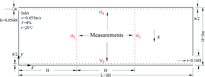

  

  Configuration, boundary condition setup and measurements of FC case

• (2) Prescribe proper boundary conditions including inlet, outlet, and four walls [iso-thermal case only: no temperature];

• (3) Select a turbulence model: the standard k-ε model, and, the RNG k-ε model (or similar);

• (4) Define convergence criterion: 0.1%;

• (5) Set iteration: at least 2000 steps for steady simulation;

• (6) Determine proper grid resolution with local refinement: at least 500,000 cells.

Cases to Be Simulated:

• (1) Test different outlet boundary condition settings (e.g., given V, P, or fully developed);

• (2) Test two turbulence models of choice using the most suitable outlet setting.

Report:

• (1) Case descriptions: description of the cases

• (2) Simulation details: computational domain, grid cells, convergence status

  • Figure of the grid used (on X-Y plane);

  • Figure of simulation convergence records.

• (3) Result and analysis

  • Figure of flow vectors;

  • Figure of pressure contours;

  • Figure of velocity contours;

  • Evaluate the influences of outlet boundary condition on simulation;

  • Evaluate the influences of turbulence model on simulation;

  • Validate the simulations with experimental data (Nielsen 1990).

• (4) Conclusions (findings, result implications, CFD experience and lessons, etc.)

References

Chen Q (1988) Indoor airflow, air quality and energy consumption of buildings. Ph.D. Thesis, Delft University of Technology, The Netherlands
Chen Q, Moser A (1991) Simulation of a multiple-nozzle diffuser. In Proceedings of the 12th AIVC conference on air movement and ventilation control within buildings, vol 2. Ottawa, Canada, pp 1–13
Launder BE, Sharma BI (1974) Application of the energy dissipation model of turbulence to the calculation of flow near a spinning disk. Lett Heat Mass Transf 1:131–138
Launder BE, Spalding DB (1974) The numerical computation of turbulent flows. Comput Methods Appl Mech Energy 3:269–289
Nielsen PV (1990) Specification of a two-dimensional test case. International energy agency
Rodi W (1991) Experience with two-layer models combining the K-epsilon model with a one-equation model near the wall. AIAA, Aerospace Sciences Meeting, 29th, Reno, NV, Jan. 7–10, 13 p
Srebric J, Chen Q (2002) Simplified numerical models for complex air supply diffusers. HVAC&R Res 8(3):277–294
Zhai Z, Chen Q (2004) Numerical determination and treatment of convective heat transfer coefficient in the coupled building energy and CFD simulation. Build Environ 39(8):1001–1009
Author information
Authors and Affiliations
Corresponding author