Case Study I: Tuning Random Forest (Ranger)

Abstract

This case study gives a hands-on description of Hyperparameter Tuning (HPT) methods discussed in this book. The Random Forest (RF) method and its implementation ranger was chosen because it is the method of the first choice in many Machine Learning (ML) tasks. RF is easy to implement and robust. It can handle continuous as well as discrete input variables. This and the following two case studies follow the same HPT pipeline: after the data set is provided and pre-processed, the experimental design is set up. Next, the HPT experiments are performed. The R package SPOT is used as a “datascope” to analyze the results from the HPT runs from several perspectives: in addition to Classification and Regression Trees (CART), the analysis combines results from surface, sensitivity and parallel plots with a classical regression analysis. Severity is used to discuss the practical relevance of the results from an error-statistical point-of-view. The well proven R package mlr is used as a uniform interface from the methods of the packages SPOT and SPOTMisc to the ML methods. The corresponding source code is explained in a comprehensible manner.

1 Introduction

In this case study, the hyperparameters of the RF algorithm are tuned for a classification task. The implementation from the R package ranger will be used. The data set used is the Census-Income (KDD) Data Set (CID).¹

The R package SPOTMisc provides a unifying interface for starting the hyperparameter-tuning runs performed in this book. The R package mlr is used as a uniform interface to the machine learning models. All additional code is provided together with this book. Examples for creating visualizations of the tuning results are also presented.

The hyperparameter tuning can be started as follows:

This case study deals with RF. However, any ML method from the set of available methods that were discussed in Chap. 3, i.e., $\texttt {glmnet}$, $\texttt {kknn}$, $\texttt {ranger}$, $\texttt {rpart}$, $\texttt {svm}$, and $\texttt {xgb}$, can be chosen. $\texttt {xgb}$ will be analyzed in Chap. 9.

Table 8.1 Machine-learning hyperparameter-tuning pipeline

Fig. 8.1

Overview. The hyperparameter-tuning pipeline introduced in this chapter comprehends four main steps. After the data acquisition ($\texttt {getDataCensus}$), the ML model is configured ($\texttt {getMlConfig}$) and the objective function ($\texttt {getObjf}$) is specified. The hyperparameter tuner $\texttt {SPOT}$ is called ($\texttt {spot}$) and finally, results are evaluated ($\texttt {evalParamCensus}$). The ML configuration via $\texttt {getMlConfig}$ combines the results from three subroutines, i.e., $\texttt {getMlrTask}$, $\texttt {getModelConf}$, and $\texttt {getMlrResample}$

The function $\texttt {startCensusRun}$ performs the following steps from Table 8.1:  

1 Data::

Acquisition and preparation of the CID data set. The function $\texttt {getDataCensus}$ is called to perform these steps; see Sect. 8.2.1.

2.1 Design::

The experimental design is set up. This step includes the specification of measures, the configuration of the hyperparameter tuner, and the configuration of the ML model. Calling the function $\texttt {getMlConfig}$ executes the subroutines 2.1.1 until 2.1.3:

2.1.1 Task::

Definition of a ML task. The function $\texttt {getMlrTask}$ performs this step. It results in an mlr $\texttt {task}$ object; see Sect. 8.3.2.1.

2.1.2 Config::

Hyperparameter configuration. The function $\texttt {getModelConf}$ sets up the hyperparameters of the model; see Sect. 8.3.2.2.

2.1.3 Split::

Generating training and test data. The function $\texttt {getMlrResample}$ is used here. It returns a $\texttt {list}$ with the corresponding data sets; see Sect. 8.3.2.3.

2.2 Objective::

The objective function is defined via $\texttt {getObjf}$; see Sect. 8.4.4.

3 Tuning::

The hyperparameter tuner, i.e., the function $\texttt {spot}$, is called. See Sect. 8.5.

4 Evaluation::

Evaluation on test data. To evaluate the results, the function $\texttt {evalParamCensus}$ can be used; see Sect. 8.6.2. These steps are illustrated in Fig. 8.1.

 

2 Data Description

2.1 The Census Data Set

For the investigation, we choose the CID, which is made available, for example, via the UCI ML Repository.² For our investigation, we will access the version of the data set that is available via the platform openml.org under the data record ID 45353 (Vanschoren et al. 2013). This data set is an excerpt from the current population surveys of 1994 and 1995, compiled by the U.S. Census Bureau. It contains $n=299,285$ observations with 41 features on demography and employment. The data set is comparatively large, has many categorical features with many levels, and fits well with the field of application of official statistics.

The CID data set suits our research questions well since it is comparatively large and has many categorical features. Several of the categorical features have a broad variety of levels. The data set can be easily used to generate different classification and regression problems.

The data preprocessing consists of the following steps:

• Feature 24 (instance weight $\texttt {MARSUPWT}$) is removed. This feature describes the number of persons in the population who are represented by the respective observation. This is relevant for data understanding, but should not be an input to the ML models.

• Several features are encoded as numerical (integer) variables, but are in fact categorical. For example, feature 3 (industry code $\texttt {ADTIND}$) is encoded as an integer. Since the respective integers represent discrete codes for different sectors of industry, they have no inherent order and should be encoded as categorical features.

• The data set sometimes contains NA values (missing data). These NA values are replaced before modeling. For categorical features, the most frequently observed category is imputed (mode). For integer features, the median is imputed, and for real-valued features the mean.

• As the only model investigated in this book, $\texttt {xgboost}$ is not able to work directly with categorical features. This becomes relevant for the experiments in Chap. 12. In that case (only for $\texttt {xgboost}$), the categorical data features are transferred into a dummy coding. For each category of the categorical feature, a new binary feature is created, which specifies whether an observation is of the respective category or not.

• Finally, we split the data randomly into test data (40% of the observations) and training data (60%).

In addition to these general preprocessing steps, we change the properties of the data set for individual experiments to cover our various hypotheses (esp. in Chap. 12). Arguably, we could have done this by using completely different data sets where each set covers different objects of investigation (i.e., different numbers of features or different m). We decided to stick to a single data set and vary it instead of generating new, comparable data sets with different properties. This allows us to reasonably compare results between the individual variations. This way, we generate multiple data sets that cover different aspects and problems in detail. While they all derive from the same data set (CID), they all have different characteristics: Number of categorical features, number of numerical features, cardinality, number of observations, and target variable. These characteristics can be quantified with respect to difficulty as discussed in Sect. 12.5.4.

In detail, we vary:  

Target::

The original target variable of the data set is the income class (below/above 50 000 USD). We choose age as the target variable instead. For classification experiments, $\texttt {age}$ will be discretized, into two classes: $\texttt {age}$ $< 40$ and $\texttt {age}$ $>= 40$. For regression, $\texttt {age}$ remains unchanged. This choice intends to establish comparability between both experiment groups (classification, regression).

$\texttt {cardinality}$::

The number of categories (cardinality). To create variants of the data set with different cardinality of categorical features, we merge categories into new, larger categories. For instance, for feature 35 (country of birth self PENATVTY) the country of origin is first merged by combining all countries from a specific continent. This reduces the cardinality, with 6 remaining categories (medium cardinality). For a further reduction (low cardinality) to three categories, the data is merged into the categories unknown, US, and abroad. Similar changes to other features are documented in the source code. For our experiments, this preprocessing step results in data sets with the levels of cardinality: low (up to 15 categories), medium (up to 24 categories), and high (up to 52 categories).

$\texttt {nnumericals}$::

Number of numerical features (nnumericals). To change the number of features, individual features are included or removed from the data set. This is done separately for categorical and numerical features and results in four levels for nnumericals (low: 0, medium: 4, high: 6, complete: 7).

$\texttt {nfactors}$::

Number of categorical features (nfactors). Correspondingly, we receive four levels for nfactors (low: 0, medium: 8, high: 16, complete: 33). Note, that these numbers become somewhat reduced, if cardinality is low (low: 0, medium: 7, high: 13, complete: 27). The reason is that some features might become redundant when merging categories.

$\texttt {n}$::

Number of observations (n). To vary n, observations are randomly sampled from the data set. We test five levels on a logarithmic scale from $10^4$ to $10^5$: 10 000, 17 783, 31 623, 56 234, and 100 000. In addition, we conduct a separate test with the complete data set, i.e., 299 285 observations.

 

To keep results comparable, most case studies in this book (Chaps. 9, 10, and 12) use the same data preprocessing of the CID data set. Only Chap. 12 considers several variations of the CID data set simultaneously.

Background: Implementation Details

The function $\texttt {getDataCensus}$ from the package SPOTMisc uses the functions $\texttt {setOMLConfig}$ and $\texttt {getOMLDataSet}$ from the R package OpenML, i.e., the CID can also be downloaded as follows:

While not strictly necessary, it is a good idea to set a permanent cache directory for Open Machine Learning (OpenML) data set. Otherwise, every new experiment will redownload the data set, taxing the OpenML servers unnecessarily.

Information about the 42 columns of the CID data set is shown in Table 8.2.

Table 8.2 CID data set

Table 8.3 Parameters used to get the CID data set. A detailed description can be found in Sect. 8.2.1

2.2 $\texttt {getDataCensus}$: Getting the Data from OML

The CID data set can be configured with respect to the target variable, the task, and the complexity of the data (e.g., number of samples, cardinality). The following variables are defined:

These variables will be passed to the function $\texttt {getDataCensus}$ to obtain the data frame $\texttt {dfCensus}$ (Fig. 8.2). The function $\texttt {getDataCensus}$ is used to get the OML data (from cache or from server). The arguments $\texttt {target}$, $\texttt {task.type}$, $\texttt {nobs}$, $\texttt {nfactors}$, $\texttt {nnumericals}$, $\texttt {cardinality}$ and $\texttt {cachedir}$ can be used, see Table 8.3.

The $\texttt {dfCensus}$ data set used in the case studies has 10 000 observations of 23 variables, which are shown in Table 8.4.

Table 8.4 The $\texttt {dfCensus}$ data set

Fig. 8.2

Step 1 of the hyperparameter-tuning pipeline introduced in this chapter: the data acquisition ($\texttt {getDataCensus}$) generates the data set $\texttt {dfCensus}$, which is a subset of the full CID data set presented in Table 8.2, because the parameter setting $\texttt {nobs}$ = 1e4, $\texttt {nfactors}$ = “high”, $\texttt {nnumericals}$ = “high”, and $\texttt {cardinality}$ = “high” was chosen

Attention: Outliers and Inconsistent Data

• Target: The values of the target variable are not equally balanced, because 61.27% of the values are $\texttt {TRUE}$, i.e., older than 40 years.

• The numerical variables $\texttt {num\_persons\_worked\_for\_employer}$ and $\texttt {weeks\_worked\_in\_year}$ can be treated as an integers.

• The factor $\texttt {income\_class}$ can be treated as a logical value.

• Summaries of the numerical variables:

  

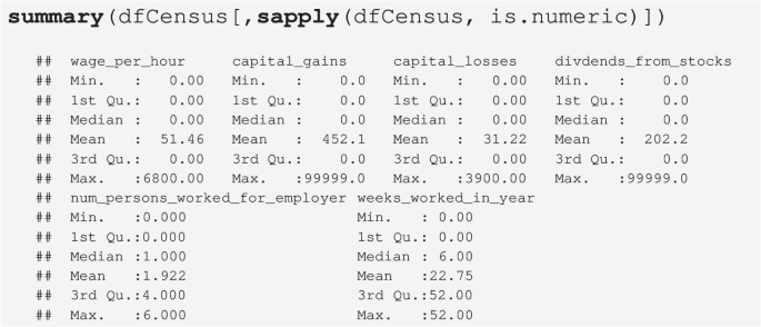
• $\texttt {capital\_gains}$ and $\texttt {divdends\_from\_stocks}$ share the same upper limit: $9.9999\times 10^{4}$, which appears to be an artificial upper limit.

• Wage per Hour: There is one entry with 6800, but income class –50000.

3 Experimental Setup and Configuration of the Random Forest Model

3.1 $\texttt {getMlConfig}$: Configuration of the ML Models

Since we are considering a binary classification problem ($\texttt {age}$, i.e., young versus old), the mlr $\texttt {task.type}$ is set to $\texttt {classif}$. Random forests ($\texttt {``ranger''}$) will be used for classification.

As a result from calling $\texttt {getMlConfig}$, the list $\texttt {cfg}$ is available. This list has 13 entries, that are summarized in Table 8.5.

Table 8.5 Configuration list with 13 entries as a result from calling $\texttt {getMlConfig}$

Fig. 8.3

Step 2 of the hyperparameter-tuning pipeline introduced in this chapter: the data acquisition ($\texttt {getMlConfig}$) generates the list $\texttt {cfg}$

3.2 Implementation Details: $\texttt {getMlConfig}$

The function $\texttt {getMlConfig}$ combines results from the following functions

• $\texttt {getMlrTask}$

• $\texttt {getModelConf}$

• $\texttt {getMlrResample}$

The functions will be explained in the following (Fig. 8.3).

3.2.1 $\texttt {getMlrTask}$: Problem Design and Definition of the Machine Learning Task

The target variable of the data set is $\texttt {age}$ (age below or above 40 years). The problem design describes target and task type, the number of observations, as well as the number of factorial, numerical, and cardinal variables. The data seed can also be specified here.

The function $\texttt {getMlrTask}$ is an interface to the function $\texttt {makeClassifTask}$ from the mlr package. The resulting $\texttt {task}$ “encapsulates the data and specifies—through its subclasses—the type of the task. It also contains a description object detailing further aspects of the data.” (Bischl et al. 2016).

Background: getMlrTask Implementation

The data set $\texttt {dfCensus}$ is passed to the function $\texttt {getMlrTask}$, which computes an mlr $\texttt {task}$ as shown below:

Because the function $\texttt {getMlrTask}$ generates an mlr Task instance, its elements can be accessed with mlr methods, i.e., functions from mlr can be applied to the Task $\texttt {task}$. For example, the feature names that are based on the data can be obtained with the mlr function $\texttt {getTaskFeatureNames}$ as follows:

The Task $\texttt {task}$ provides the basis for the the information that is needed to perform the hyperparameter tuning. Additional information is generated by the functions $\texttt {getModelConf}$, that is presented next.

3.2.2 $\texttt {getModelConf}$: Algorithm Design—Hyperparameters of the Models

The function $\texttt {getModelConf}$ generates a list with the entries $\texttt {learner}$, $\texttt {tunepars}$, $\texttt {defaults}$, $\texttt {lower}$, $\texttt {upper}$, $\texttt {type}$, $\texttt {fixpars}$, $\texttt {factorlevels}$, $\texttt {transformations}$, $\texttt {dummy}$, $\texttt {relpars}$, $\texttt {task}$, and $\texttt {resample}$ that are summarized in Table 8.5.

The ML configuration list $\texttt {modelCfg}$ contains information about the hyperparameters of the $\texttt {ranger}$ model; see Table 8.6.

Table 8.6 Ranger hyperparameter. $N_{\text {Feats}}$ denotes the output from $\texttt {getTaskNFeats(task)}$

Background: Model Information from getModelConf

The information about the $\texttt {ranger}$ hyperparameters, their ranges and types, is compiled as a list. It is accessible via the function $\texttt {getModelConf}$. This function manages the information about the $\texttt {ranger}$ model as follows:

Similar information is provided for every ML model. Note: This list is independent from mlr, i.e., it does not use any mlr classes.

3.2.3 $\texttt {getMlrResample}$: Training and Test Data

The function $\texttt {getMlrResample}$ is the third and last subroutine used by the function $\texttt {getMlConfig}$. It takes care of the partitioning of the data into training data, $X^{(\text {train})}$, and test data, $X^{(\text {test})}$, based on prop. The function $\texttt {getMlrResample}$ from the package SPOTMisc is an interface to the mlr function $\texttt {makeFixedHoldout}$ $\texttt {Instance}$, which generates a fixed holdout instance for resampling.

$\texttt {rsmpl}$ specifies the training data set, $X^{(\text {train})}$, which contains $\texttt {prop}$ $= 2/3$ of the data and the testing data set, $X^{(\text {test})}$ with the remaining $1 - \texttt {prop} = 1/3$ of the data. It is implemented as a list, the central components are lists of indices to select the members of the corresponding train or test data sets.

Background: getMlrResample

Information about the data split are stored in the $\texttt {cfg}$ list as $\texttt {cfg\$resample}$. They can also be computed directly using the function $\texttt {getMlrResample}$. This function computes an mlr $\texttt {resample}$ instance generated with the function $\texttt {makeFixedHoldoutInstance}$.

The function $\texttt {getMlrResample}$ instantiated an mlr resampling strategy object from the class $\texttt {makeResampleInstance}$. This mlr class encapsulates training and test data sets generated from the data set for multiple iterations. It essentially stores a set of integer vectors that provide the training and testing examples for each iteration. (Bischl et al. 2016). The first entry, $\texttt {desc}$, describes the split between training and test data and its properties, e.g., what to predict during resampling: $\texttt {``train''}$, $\texttt {``test''}$ or $\texttt {``both''}$ sets. The second entry, $\texttt {size}$, stores the size of the data set to resample. The third and fourth elements are lists with the training and test indices, i.e., for 6666 indices for the $X^{(\text {train})}$data set and 3334 indices for the $X^{(\text {test})}$data set. These indices will be used for all iterations. The last element is optional and encodes whether specific iterations “belong together” (Bischl et al. 2016).

Important: Training and Test Data

mlr ’s function $\texttt {resample}$ requires information about the test data, because it manages the train and test data partition internally. Usually, it is considered “best practice” in ML not to pass the test set to the ML model. To the best of our knowledge, this is not possible in mlr.

Therefore, the full data set (training and test data) with $\texttt {nobs}$ $= 10^{4}$ observations is passed to the $\texttt {resample}$ function. Because mlr is an established R package, we trust the authors that mlr keeps training and test data separately.

An additional problem occurs if the test data set, $X^{(\text {test})}$, contains data with unknown labels, i.e., factors with unknown levels. If these unknown levels are passed to the trained model, predictions cannot be computed.

4 Objective Function (Model Performance)

4.1 Performance Measures

The evaluation of hyperparameter values requires a measure of quality, which determines how well the resulting models perform. For the classification experiments, we use Mean Mis-Classification Error (MMCE) as defined in Eq. (2.2). The hyperparameter tuner Sequential Parameter Optimization Toolbox (SPOT) uses these MMCE on the test data set to determine better hyperparameter values.

In addition to MMCE, we also record run time (overall run time of a model evaluation, run time for prediction, run time for training). To mirror a realistic use case, we specify a fixed run time budget for the tuner. This limits how long the tuner may take to find potentially optimal hyperparameter values.

For a majority of the models, the run time of a single evaluation (training + prediction) is hard to predict and may easily become excessive if parameters are chosen poorly. In extreme cases, the run time of a single evaluation may exceed drastically the planned run time. In such a case, there would be insufficient time to test different hyperparameter values. To prevent this, we specify a limit for the run time of a single evaluation, which we call $\texttt {timeout}$. When the $\texttt {timeout}$ is exceeded by the model, the evaluation will be aborted. During the experiments, we set the timeout to a twentieth of the tuner’s overall run time budget.

Exceptions are the experiments with Decision Tree (DT) ($\texttt {rpart}$): Since $\texttt {rpart}$ evaluates extremely quickly, (in our experiments: usually much less than a second) the timeout is not required. In fact, using the $\texttt {timeout}$ would add considerable overhead to the evaluation time in this case.

The HPT task can be parallelized by specifying $\texttt {nthread}$ values larger than one. Only one thread was used in the experiment. In addition to Root Mean Squared Error (RMSE) and MMCE, we also record run time (overall run time of a model evaluation, run time for prediction, run time for training). Several alternative metrics can be specified.

Example: Changing the loss function

For example, $\texttt {logloss}$ can be selected as follows:

4.2 Handling Errors

If the evaluation is aborted (e.g., due to $\texttt {timeout}$ or in case of some numerical instability), we still require a quality value to be returned to the tuner, so that the search can continue. This return value should be chosen, so that, e.g., additional evaluations with high run times are avoided. At the same time, the value should be on a similar scale as the actual quality measure, to avoid a deterioration of the underlying surrogate model. To achieve this, we return the following values when an evaluation aborts.

• Classification: Model quality for simply predicting the mode of the training data.

• Regression: Model quality for simply predicting the mean of the training data.

4.3 Imputation of Missing Data

The imputation of missing values can be implemented using built-in methods from mlr. These imputations are based on the hyperparameter types: factor variables will use $\texttt {imputeMode}$, integers use $\texttt {imputeMedian}$, and numerical values use $\texttt {imputeMean}$.

Important: Imputation

There are two situations when imputation can be applied:

• 1. Missing data, i.e., CID data are incomplete. This imputation can be handled by the mlr methods described in this section.

• 2. Missing results, i.e., performance values of the ML method such as loss or accuracy. This imputation can be handled by $\texttt {spot}$.

4.4 $\texttt {getObjf}$: The Objective Function

After the ML configuration is compiled via $\texttt {getMlConfig}$, the objective function has to be generated.

The $\texttt {getObjf}$ compiles information from the $\texttt {cfg}$ and information about the budget ($\texttt {timeout}$) (Fig. 8.4).

Fig. 8.4

Step 3 of the hyperparameter-tuning pipeline introduced in this chapter: ($\texttt {getObjf}$) generates the function $\texttt {objf}$

Background: getObjf as an Interface to mlr’s resample function

Note, in addition to hyperparameter information, $\texttt {cfg}$ includes information about the mlr $\texttt {task}$. $\texttt {getObjf}$ calls the mlr function $\texttt {makeLearner}$. The information is used to execute the $\texttt {resample}$ function, which fits a model specified by $\texttt {learner}$ on a $\texttt {task}$. Predictions and performance measurements are computed for all training and testing sets specified by the resampling method (Bischl et al. 2016).

A simplified version that implements the basic elements of the function $\texttt {getObjf}$, is shown below. After the parameter names are set, the parameter transformations are performed and the complete set of parameters is compiled: this includes converting integer levels to factor levels for categorical parameters, setting fixed parameters (which are not tuned, but are also not set to default value), and setting parameters in relation to other parameters (e.g., minbucket relative to minsplit). Next, the learner $\texttt {lrn}$ is generated via mlr ’s function $\texttt {makeLearner}$, and the measures are defined. Here, the fixed set $\texttt {mmce}$, $\texttt {timeboth}$, $\texttt {timetrain}$, and $\texttt {timepredict}$ are used. After setting the Random Number Generator (RNG) seed, the mlr function $\texttt {resample}$ is called. The function $\texttt {resample}$ fits a model specified by the learner on a task and calculates performance measures for all training sets, $X^{(\text {train})}$, and all test sets, $X^{(\text {test})}$, specified by the resampling instance $\texttt {config\$resample}$ that was generated with the function $\texttt {getMlrResample}$ as described in Sect. 8.3.2.3.

The return value, $\texttt {res}$, of the objective function generated with $\texttt {getObjf}$ was evaluated on the test set, $X^{(\text {test})}$.

No explicit validation set, $X^{(\text {val})}$, is defined during the HPT procedure.

Importantly, randomization is handled by $\texttt {spot}$ by managing the $\texttt {seed}$ via $\texttt {spot}$ ’s $\texttt {seedFun}$ argument. The seed management guarantees that two different hyperparameter configurations, $\lambda _i$ and $\lambda _j$, are evaluated on the same test data $X^{(\text {test})}$. But if the same configuration is evaluated a second time, it will receive a new test data set.

5 $\texttt {spot}$: Experimental Setup for the Hyperparameter Tuner

The R package SPOT is used to perform the actual hyperparameter tuning (optimization). The hyperparameter tuner itself has parameters such as kind and size of the initial design, methods for handling non-numerical data (e.g., $\texttt {Inf}$, $\texttt {NA}$, $\texttt {NaN}$), the surrogate model and the optimizer, search bounds, number of repeats, methods for handling noise.

Because the generic SPOT setup was introduced in Sect. 4.5, this section highlights the modifications of the generic setup that were made for the ML runs.

The third step of the hyperparameter-tuning pipeline as shown in Fig. 8.5 starts the SPOT hyperparameter tuner.

Fig. 8.5

The hyperparameter-tuning pipeline: the hyperparameter tuner $\texttt {SPOT}$ is called ($\texttt {spot}$)

The result from the $\texttt {spot}$ run is the $\texttt {result}$ list, which can be written to a file. The full R code for running this case study is shown Sect. 8.10 and the SPOT parameters are listed in Table 8.7.

Table 8.7 SPOT parameters used for ML hyperparameter tuning. Parameters, that are implemented as lists are described in Table 8.8. This table shows only parameters that were modified for the ML and Deep Learning (DL) hyperparameter-tuning tasks. The full list is shown in Table 4.2

Table 8.8 SPOT control list parameters used for ML hyperparameter tuning. This table shows only parameters that were modified for the ML and DL hyperparameter-tuning tasks. The full list is shown in Table 4.2

Background: Implementation details of the function spot

The initial design is created by Latin Hypercube Sampling (LHS) (Leary et al. 2003). The size of that design (number of sampled configurations of hyperparameters) corresponds to $2 \times k$. Here, k is the number of hyperparameters.

6 Tunability

The following analysis is based on the results from the $\texttt {spot}$ run, which are stored in the data folder of this book. They can be loaded with the following command:

Now the information generated with $\texttt {spot}$, which was stored in the $\texttt {result}$ list as described in Sect. 8.5, is available in the R environment.

6.1 Progress

The function $\texttt {prepareProgressPlot}$ generates a data frame that can be used to visualize the hyperparameter-tuning progress. The data frame can be passed to $\texttt {ggplot}$. Figure 8.6 visualizes the progress during the $\texttt {ranger}$ hyperparameter-tuning process described in this study.

Fig. 8.6

Ranger: Hyperparameter-tuning progress. The red dashed line denotes the best value found by the initial design. The blue dashed line represents the best value from the whole run

After 60 min, 582 $\texttt {ranger}$ models were evaluated. Comparing the worst configuration that was observed during the HPT with the best, a 25.8442 % reduction was obtained. After the initial phase, which includes 20 evaluations, the smallest MMCE reads 0.179964. The dotted red line in Fig. 8.6 illustrates this result. The final best value reads 0.1712657, i.e., a reduction of the MMCE of 4.8333%. These values, in combination with results shown in the progress plot (Fig. 8.6) indicate that a quick HPT run is able to improve the quality of the $\texttt {ranger}$ method. It also indicates, that increased run times do not result in a significant improvement of the MMCE.

Attention

These results do not replace a sound statistical comparison, they are only indicators, not final conclusions.

6.2 $\texttt {evalParamCensus}$: Comparing Default and Tuned Parameters on Test Data

As a comparison basis, an additional experiment for the $\texttt {ranger}$ model where all hyperparameter values remain at the model’s default settings and an additional experiment where the tuned hyperparameters are used, is performed. In these cases, a $\texttt {timeout}$ for evaluation was not set. Since no search takes place, the overall run time for default values is anyways considerably lower than the run time of $\texttt {spot}$. The final comparison is based on the classification error as defined in Eq. (2.2). The motivation for this comparison is a consequence of the tunability definition; see Definition 2.26.

To understand the impact of tuning, the best solution obtained is evaluated for n repeats and compared with the performance (MMCE) of the default settings. A power analysis, as described in Sect. 5.6.5 is performed to estimate the number of repeats, n.

The corresponding values are shown in Table 8.9. The function $\texttt {evalParamCensus}$ was used to perform this comparison. Results from the evaluations on the test data for the default and the tuned hyperparameter configurations are saved to the corresponding files.

Default and tuned results for the $\texttt {ranger}$ model are available in the supplementary data folder as $\texttt {rangerDefaultEvaluation.RData}$ and $\texttt {ranger00001Evaluation.RData}$, respectively.

Important:

As explained in Sect. 8.4.4, no explicit validation set, $X^{(\text {val})}$, is defined during the HPT procedure. The response surface function $\psi ^{(\text {test})}$ is optimized. But, since we can generate new data sets, (X, Y) randomly, the comparison is based on several, randomly generated samples.

Background: Additional Scores

The scores are stored as a matrix. Attributes are used to label the measures. In addition to $\texttt {mmce}$, the following measures are calculated for each repeat: $\texttt {accuracy}$, $\texttt {f1}$, $\texttt {logLoss}$, $\texttt {mae}$, $\texttt {precision}$, $\texttt {recall}$, and $\texttt {rmse}$. These results are stored in the corresponding $\texttt {RData}$ files.

Hyperparameters of the default and the tuned configurations are shown in Table 8.9.

Table 8.9 Comparison of default and tuned hyperparameters of the $\texttt {``ranger''}$ model. r.u.f. denotes respect.unordered.factors and s.f sample.fraction

Fig. 8.7

Comparison of ranger algorithms with default (D) and tuned (T) hyperparameters. Classification error (MMCE). Vertical lines mark quantiles (0.25, 0.5, 0.75) of the corresponding distribution. Numerical values are shown in Table 8.9

The corresponding R code for replicating the experiment is available in the code folder. The result files can be loaded and the violin plot of the obtained MMCE can be visualized as shown in Fig. 8.7. It can be seen that the tuned solutions provide a better MMCE on the holdout test data set $(X,Y)^{(\text {test})}$.

7 Analyzing the Random Forest Tuning Process

To analyze effects and interactions between hyperparameters of the $\texttt {ranger}$ model as defined in Table 8.6, a simple regression tree as shown in Fig. 8.8 can be used.

Fig. 8.8

Regression tree. Case study I. Ranger

The regression tree supports the observations, that hyperparameter values for sample.fraction, num.trees, and respect.unordered.factors, have the largest effect on the MMCE.

b!

	sample.fraction	num.trees	respect.unordered.factors	mtry	replaRce
1	0.010297452	0.006007073	0.0015083938	0.0013354262	0.00015087878

Parallel plots visualize relations between hyperparameters. The SPOTMisc function $\texttt {ggparcoordPrepare}$ provides an interface from the data frame $\texttt {result}$, which is returned from the function $\texttt {spot}$, to the function $\texttt {ggparcoord}$ from the package GGally. The argument $\texttt {probs}$ specifies the quantile probabilities for categorizing the result values. In Fig. 8.9, quantile probabilities are set to $\texttt {c(0.25, 0.5, 0.75)}$. Specifying three values results in four categories with increasing performance, i.e., the first category (0–25%) contains poor results, the second and the third categories, 25–50 % and 50 to 75%, respectively, contain mediocre values, whereas the last category (75–100%) contains the best values.

Fig. 8.9

Parallel plot of results from the ranger hyperparameter-tuning process. num.trees ($x_1$), mtry ($x_2$), sample.fraction ($x_3$), replace ($x_4$), and respect.unordered.factors ($x_5$) are shown. Best configurations in green

Fig. 8.10

Sensitivity plot (best). num.trees ($x_1$), mtry ($x_2$), sample.fraction ($x_3$), replace ($x_4$), and respect.unordered.factors ($x_5$) are shown

In addition to labeling the best configurations, the worst configurations can also be labeled.

Results from the $\texttt {spot}$ run can be passed to the function $\texttt {plotSenstivity}$, which generates a sensitivity plot as shown in Fig. 8.10. There are basically two types of sensitivity plots that can be generated with $\texttt {plotSenstivity}$: using the argument $\texttt {type = ``best''}$, the best hyperparameter configuration is used. Alternatively, using $\texttt {type = ``agg''}$, simulations are performed over the range of all hyperparameter settings. Note, the second option requires additional computations and depends on the simulation output, which is usually non-deterministic. Output from the second option is shown in Fig. 8.11.

If the results from using the argument $\texttt {type = ``best''}$ and $\texttt {type = ``agg''}$ are qualitatively similar, only the plot based on $\texttt {type = ``best''}$ will be shown in the remainder of this book. Parallel plots will be treated in a similar manner. Source code for generating all plots is provided.

Fig. 8.11

Ranger: Sensitivity plot (aggregated). num.trees ($x_1$), mtry ($x_2$), sample.fraction ($x_3$), replace ($x_4$), and respect.unordered.factors ($x_5$) are shown

SPOT provides several tools for the analysis of interactions. Highly recommended is the use of contour plots as shown in Fig. 8.12.

Fig. 8.12

Surface plot: $x_3$ (sample.fraction) plotted against $x_1$ (numtrees)

Finally, a simple linear regression model can be fitted to the data. Based on the data from SPOT’s $\texttt {result}$ list, the hyperparameters $\texttt {replace}$ and $\texttt {respect.}$ $\texttt {unordered.factors}$ are converted to $\texttt {factors}$ and the R function $\texttt {lm}$ is applied. The summary table is shown below.

Although this linear model requires a detailed investigation (a mispecification analysis is necessary), it also is in accordance with previous observations that hyperparameters sample.fraction, num.trees, and respect.unordered.factors have significant effects on the loss function.

Results indicate that sample.fraction is the dominating hyperparameter. Its setting has the largest impact on $\texttt {ranger}$ ’s performance. For example, the sensitivity plot Fig. 8.10 shows that small sample.fraction values improve the performance. The larger values clearly improve the performance. The regression tree analysis (see Fig. 8.8) supports this hypothesis, because sample.fraction is the root node of the tree and values smaller than 0.48 are recommended. Furthermore, the regression tree analysis indicates that additional improvements can be obtained if the num.trees is greater equal 2. These observations are supported by the parallel plots and surface plots, too. The linear model can be interpreted in a similar manner.

8 Severity: Validating the Results

Now, let us proceed to analyze the statistical significance of the achieved performance improvement. The results from the pre-experimental runs indicate that the difference is $\bar{x} =$ 0.0057. As this value is positive, for the moment, let us assume that the tuned solution is superior. The corresponding standard deviation is $s_d =$ 0.0045. Based on Eq. 5.14, and with $\alpha =$ 0.05, $\beta =$ 0.2, and $\Delta =$ 0.005 let us identify the required number of runs for the the full experiment using the $\texttt {getSampleSize}$ function.

For a relevant difference of 0.005, approximately 10 runs per algorithm are required. Since, we evaluated for 30 repeats, we can now proceed to evaluate the severity and analyse the performance improvement achieved through tuning the parameters of the $\texttt {ranger}$.

The summary result statistics is presented in Table 8.10. The decision based on p-value is to reject the null hypothesis, i.e., the claim that the tuned parameter setup provides a significant performance improvement in terms of MMCE is supported. The effect size suggests that the difference is of larger magnitude. For the chosen $\Delta =$ 0.005, the severity value is at 0.8 and thus it strongly supports the decision of rejecting the $H_0$. The severity plot is shown in Fig. 8.13. Severity shows that performance difference smaller than or equal to 0.005 are well supported.

Table 8.10 Case study I: result analysis

Fig. 8.13

Tuning Random Forest. Severity of rejecting H0 (red), power (blue), and error (gray). Left: the observed mean $\bar{x} =$ 0.0057 is larger than the cut-off point $c_{1-\alpha } =$ 0.0014 Right: The claim that the true difference is as large 0.005 are well supported by severity. However, any difference larger than 0.005 is not supported by severity

9 Summary and Discussion

The analysis indicates that hyperparameter sample.fraction has the greatest effect on the algorithm’s performance. The recommended value of sample.fraction is 0.1416, which is much smaller than of 1.

This case study demonstrates how functions from the R packages mlr and SPOT can be combined to perform a well-structured hyperparameter tuning and analysis. By specifying the time budget via $\texttt {maxTime}$, the user can systematically improve hyperparameter settings. Before applying ML algorithms such as RF to complex classification or regression problems, HPT is recommended. Wrong hyperparameter settings can be avoided. Insight into the behavior of ML algorithms can be obtained.

10 Program Code

Program Code