Use of Open-Source Tools for Imaging and Recording Phenotypic Traits of a Coffee (Coffea arabica L.) Mutant Population

Abstract

Mutation breeding in Coffea arabica offers a powerful tool to induce novel genetic variability for breeding and genetic studies. The success of a mutation breeding program depends largely on the ability to screen large populations for target traits. There is also a need to accurately record induced mutant traits at the individual plant level. Comprehensive phenotyping requires measuring and tracking traits of interest during the crop growth cycle and subsequent generations. Therefore, efficient and accurate data collection and recording of traits is essential, both at the individual plant level and populations. In recent years, various high-throughput plant phenotyping platforms have been developed. However, these are typically proprietary, and/or require costly infrastructures. In this chapter we illustrate the use of Field Book and ImageJ, two public domain software tools, for phenotyping and documenting growth and yield traits of a greenhouse-grown Arabica coffee mutant population. Example data of M₁ and M₂ mutant phenotypes induced through EMS and gamma-ray mutagenesis are presented. We further demonstrate the use of these tools for quantifying the canopy of mutants and non-mutagenized controls. These tools can be more widely applied to other visual phenotypes including plant or tissue responses to biotic or abiotic stresses. The use of free, open-access tools for integrating electronic data recording with image processing can greatly improve the efficiency, precision and speed of data collection for screening large mutant populations and is especially useful in resource-limiting settings.

1 Introduction

Coffee (Coffea spp.) is an indispensable source of income in Asia, Africa, South and Central America. It is ranked among the world’s most valuable export commodities, on which more than 125 million people in the coffee growing areas derive their income directly or indirectly (FAO 2015). C. arabica contributes about 75% of the world coffee production due to its superior cup quality and aromatic characteristics. C. arabica has a unique biology compared to other species in the genus Coffea because it is a self-fertile, allotetraploid (2n = 4x = 44) species while almost all other coffee species are diploids (2n = 2x = 22) and generally self-incompatible (Carvalho et al. 1991). Due to its reproductive biology, C. arabica varieties tend to remain genetically stable. However, C. arabica varieties are typically low yielding and highly susceptible to a myriad pests and diseases and abiotic stresses, including Coffee Leaf Rust (CLR). Genetic improvement of C. arabica to withstand the afore mentioned constraints and with higher yield through classical breeding is laborious and can require up to 25–30 years to release an improved variety (Lashermes et al. 1996, 2009).

Mutation breeding offers a powerful tool to enhance genetic variation in the C. arabica gene pool which is very narrow. Random mutagenesis has been used in different crops to induce novel agronomic traits that were absent in their primary gene pool (Ulukapi and Nasircilar 2018). Induced mutagenesis can enhance stable, genetic variability not only in seed but also in vegetatively propagated plants (Jain 2005; Pathirana et al. 2009). Major traits improved through mutation-assisted breeding include plant architecture, early flowering and maturity, yield and quality traits, and tolerance to pests and diseases (Pathirana 2011; FAO/IAEA 2018). For a successful coffee mutation breeding program, phenotyping large mutant populations is paramount. Likewise, it is important to identify, and document induced mutant phenotypes at the individual plant level. Comprehensive phenotyping requires that traits of interest can be accurately and rapidly measured and documented during the crop growth cycle and subsequent generations (Sabina 2022). Recent technological advances have enabled accurate, high-throughput plant phenotyping. Commercial and open-source digital phenotyping technologies and methods have been developed to increase the precision and speed of data collection and analysis useful for plant breeders. However, high-throughput phenotyping methods typically require highly automated and sophisticated systems for image acquisition and analysis. Also, high-throughput technologies require significant infrastructural investment in the field or greenhouse facilities. The use of simple image capture tools such as manually operated cameras and downstream open-source image analysis tools such as ImageJ, Fiji and MATLAB provide affordable alternatives (Hartmann et al. 2011; Schindelin et al. 2012; Singh et al. 2017). In recent years several open-access applications for data recording have been developed. Examples include Field Book, an open-source application for taking phenotypic notes (Rife and Poland 2014), OneKK, an app designed to analyze seed lots, Coordinate, an open-source Android app used to collect and organize data into a predefined grid (Prasad et al. 2018) and Open Data Kit (ODK) for seed tracking (Ouma et al. 2019). Such public domain software tools facilitate a digital migration from manual methods of data capture and recording that are associated with unstandardised data that is difficult to process for analysis (Mechael 2009).

In this chapter, we illustrate the use of two public domain software tools, Field Book and ImageJ, for phenotyping and documenting growth and yield component traits of C. arabica M₁ and M₂ populations and plants developed and maintained in the greenhouse of the FAO/IAEA Plant Breeding and Genetics Laboratory in Seibersdorf, Austria. These tools are simple, user-friendly and especially useful for plant scientists, breeders or data collectors in resource-limiting environments where advanced, high-throughput phenotyping facilities and/or expertise is missing.

2 Materials

2.1 Establishment of the C. Arabica Mutant Populations

• 1. Acclimatised/hardened six-months old coffee mutagenized seedlings (see Note 1).

• 2. Greenhouse.

• 3. Peat soil.

• 4. Sand.

• 5. Potting mixer (shovel or spade).

• 6. 5-L pots.

• 7. Plastic labels/tags.

• 8. Marker pens/Pencils.

• 9. Water supply system.

• 10. Watering can, horse pipe or drip irrigation system.

• 11. Complex fertilizers for instance ENTEC^® (NPK- 14 + 7 + 17(+ 2 + 9) + 0.02 B + 0.01 Zn; Eurochem).

• 12. Systemic pesticides (fungicides and insecticides).

• 13. Pesticide sprayer.

• 14. Chemical protective gear.

2.2 Phenotyping of the Mutant Populations

• 1. Electronic data collection tool (Android tablet/phone) or data sheet.

• 2. Field Book application.

• 3. Trait list and trait descriptors.

• 4. Rulers (30, 200 cm).

• 5. Vernier calliper.

• 6. Camera and camera stand.

• 7. Pencil.

• 8. Permanent markers.

• 9. Tags/labels.

• 10. Computer/workstation.

2.3 Data Analysis Tools

• 1. ImageJ software (digital image analysis).

• 2. Excel spreadsheet.

• 3. Statistical software (any software that you are familiar with).

3 Methods

3.1 Establishing the M₁ Mutant Population

• 1. Clean and disinfect the greenhouse at least one week before planting to eliminate potential pests and disease pathogens that may affect coffee plants.

• 2. Obtain well acclimatized/hardened M₁ seedlings (see Chap. “Chemical Mutagenesis of Mature Seed of Coffea arabica L. var. Venecia Using EMS”, Note 1 and Fig. 1a).

  Fig. 1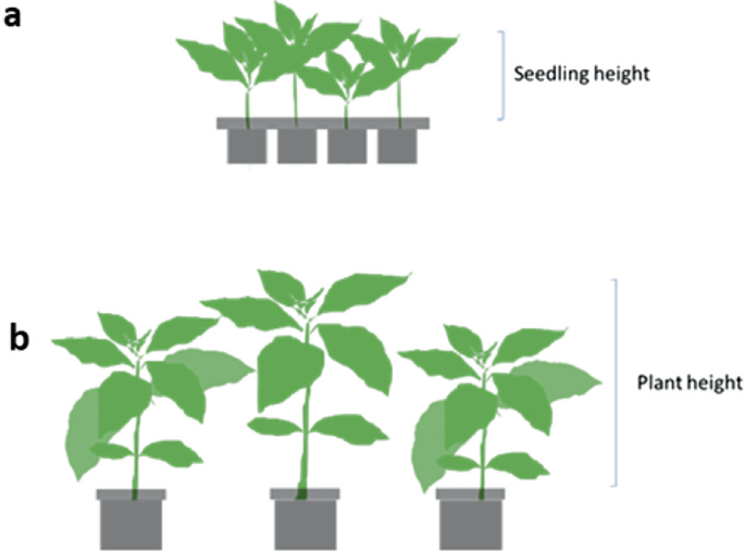

  

  Developmental stages of coffee mutants. a Coffee seedlings with 4–5 true leaves, ready for transplanting. Just before transplanting, data can be recorded on traits like number of leaves, size of canopy and leaf dimensions (leaf length and leaf width) (see Chap. “Chemical Mutagenesis of Mature Seed of Coffea arabica L. var. Venecia Using EMS”). b Mutant plants established in pots at about six months after transplanting. Growth traits including plant height can be measured to monitor plant growth

• 3. Mix the potting medium containing peat soil and sand (3:1 v/v) at pH 5–6.

• 4. Distribute uniformly the potting medium into clean 5 L pots.

• 5. Carefully remove the hardened seedlings from the small container pots and transplant them in the 5 L pots (see Note 2 and Fig. 1b).

• 6. Do not fill the pots completely with the potting mix, leave about 3 cm depth.

• 7. During transplanting, handle treatments separately to avoid errors that may arise due to cross mixing.

• 8. Label the pots accordingly with the information about the genotype, mutagen concentration or dose and treatment date. Ensure that each seedling bears a unique identifier since it is an independent event.

• 9. Arrange the pots randomly into blocks in a complete randomised design (CRD) with uniform spacing of at least 30 cm within blocks and 100 cm between blocks (see Note 3).

• 10. During plant growth, monitor the pots and design an appropriate watering regime, usually three times a week, depending on climatic conditions.

• 11. Periodically apply fertilizers (see Note 4).

• 12. Inspect plants regularly for pests and diseases, apply appropriate and recommended (systemic) pesticides (see Note 5).

3.2 Phenotypic Characterisation of the M₁ Mutant Population

3.2.1 Electronic Phenotyping Tools

• 1. Use the Field Book application to record growth and yield traits (see Note 6 and Fig. 2).

  Fig. 2

  

  Schematic representation of the steps taken while using Field Book application for data collection on a coffee mutant population. a The overview of the layout of the field (import file) displaying information on coffee mutant labels only. No trait information is required. b Field Book logo. c Option for importing the experimental layout as a field into the application. d Option to input and define trait. e Appearance of the coffee traits as defined in the application. f Option to begin data collection. g An interface during data collection. It displays the trait (e.g., plant height), plant ID (e.g. Ca-2020–001 Gy 20) information as previously determined. Forward and backward arrows guide data collection. h Option to export data after collection for storage. i Selected procedure to export the data after collection

• 2. Install the Field Book on your Android device, e.g., from Google Play Store (Fig. 2b).

• 3. Design an experimental layout in Excel on your laptop (Fig. 2a).

• 4. Import the experimental layout in the Field Book application into the import folder.

• 5. To activate the experimental layout file, open the application on your device and import the file as a field from local storage (Fig. 2c).

• 6. Add your traits of interest into the Field Book (Fig. 2d, e). The trait list and trait description should be prepared beforehand (IPGRI 1996).

• 7. Define your traits as numeric, categorical, percentage, date or text (in case you need to make notes/comments during data collection).

• 8. Data collection can start immediately (Fig. 2f). No internet connection is required.

• 9. Use forward/backward arrows to move to the next trait or plot and vice versa (Fig. 2g). If barcodes are used in the experiment, scanning barcodes (also provided in the application) is much better and faster than arrows.

• 10. In case of many traits, select or activate traits whose data is ready before you start data collection, since some traits appear before others, for instance flowers vs fruits.

• 11. After data collection, one can turn off the device. The entered data remains intact, you can resume from where you stopped upon the next data collection.

• 12. To archive the data, connect the device to the internet and export data (Fig. 2h, i).

• 13. The file name is automatically generated and can be changed as preferred. Save the data in the preferred destination.

• 14. The exported data is received as an Excel (csv) file containing all the traits as column headers, with the corresponding data records for every plant/plot/block etc. (Fig. 3).

  Fig. 3

  

  A screenshot of the exported data file from the Field Book application for the coffee mutant population. The file is retrieved as an Excel file (csv). Compared to the import file, the extra columns show traits with the corresponding data

3.2.2 Measurement of Growth Traits

• 1. Open the Field Book application on your device for data recording.

• 2. Use non-destructive methods to phenotype your mutant population.

• 3. At transplanting, assess the seedlings for any visible morphological characteristics, such as leaf colour and shape (Fig. 4).

  Fig. 4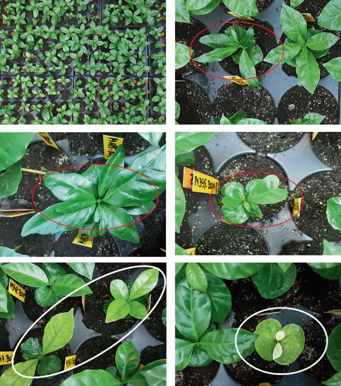

  

  M₂ seedlings five months after sowing. Abnormal phenotypes were identified at early stages of seedling development. The red-circled seedlings indicate aberrant leaf shapes. The seedlings within white circles show yellowing, an indicator of chlorophyll deficiencies

• 4. If possible, fix the camera (Fig. 5) and take aerial pictures of the seedling (Chap. “Chemical Mutagenesis of Mature Seed of Coffea arabica L. var. Venecia Using EMS” and Fig. 6).

  Fig. 5

  

  Image capture of the seedlings at transplanting. a Camera stand with three support stands. b Camera fixed in one position to capture all images. c Acclimatized potted seedling ready for transplanting

  Fig. 6

  

  Example images of M₁ seedlings captured using the fixed camera setting for ImageJ analysis (see Chap. “Chemical Mutagenesis of Mature Seed of Coffea arabica L. var. Venecia Using EMS”)

• 5. Using a ruler, measure the height of seedlings. Seedling height should be measured from the soil surface to the last apical node of the stem (Fig. 1a).

• 6. Record the number of leaves per seedling. Leaves that are less than 50% green due to senescence should not be counted.

• 7. Using a Vernier caliper, measure and record stem diameter. Measure diameter at 3 cm above the soil level for seedlings and 5 cm for mature plants.

• 8. After transplanting, monitor growth traits with intervals of at least six months. As good practice for record tracking, always record the data collection dates.

• 9. Using a calibrated 200 cm ruler, measure plant height. Like for seedlings, plant height should be measured from the soil surface to the last apical node of the stem (see Note 7 and Fig. 1b).

• 10. Score the type of plant canopy qualitatively by visual assessment using predetermined descriptors such as compact, intermediate and open canopies. The size of the canopy can be determined quantitively by image analysis using tools like ImageJ.

• 11. Count the number of branches, starting from the oldest living branch to the highest (youngest) branch.

• 12. Score the angle of insertion of branches as drooping, horizontal or spreading, and as erect or semi-erect.

• 13. Score the colour of young leaves as green, dark green, yellow, etc.

• 14. Record leaf morphology as obovate, ovate, elliptic or lanceolate.

• 15. Record the morphology of leaf margin or apex shapes as round, obtuse, acute, acuminate, apiculate or spatulate.

• 16. Measure and record the average leaf length and width from five random mature leaves (> node 3 from the terminal bud). Leaf length is measured from leaf stalk to the apex while leaf width is measured from the widest part of the leaf.

• 17. Use leaf length and width to estimate leaf area that is an important measure of light interception and consequently plant productivity.

3.2.3 Measurement of Yield Component Traits

• 1. When the plants reach reproductive maturity, inspect and monitor plants daily and record yield component traits of interest.

• 2. Record the number of days to flower bud initiation  for each plant.

• 3. Record the number of flower buds per axil. Determine the average number of buds from 10 axils, selected randomly from different nodes of different branches.

• 4. Record the number of days to flowering. This is determined from the planting date to the appearance of the first flowers.

• 5. Assess flower morphology and colour. Record any aberrations.

• 6. Record the average number of petals/corolla per flower, determined from the average of 10 flowers selected randomly from different nodes.

• 7. Measure and record the average length of petals per flower (mm), determined from 10 flowers selected randomly from different nodes.

• 8. Measure the average diameter (mm) of petals. Determine the petal diameter from the widest parts of the petals from 10 flowers selected randomly from different nodes.

• 9. Record the number of stamens/anthers per flower as the average of 10 flowers selected randomly from different nodes.

• 10. Record the length of stamens per flower (mm) as the average of 10 flowers selected randomly from different nodes.

• 11. Record the number of days or weeks to fruit/berry maturity (from bloom to harvest).

• 12. Record mature fruit colour as red, black, purple or orange.

• 13. Record fruit morphology as round, obovate or ovate.

• 14. Determine the weight of 20 mature fruits.

• 15. Measure and record fruit length (mm) as the average of five normal mature green fruits, measured using a Vernier caliper.

• 16. Measure fruit width (mm) as the average of five normal mature green fruits, measured at the widest part using a Vernier calliper.

• 17. Record the number of beans per berry, determined from five normal mature berries after de-pulping the berries.

• 18. Measure bean length (mm) as the average of five normal mature seeds.

• 19. Measure bean width (mm) as the average of five normal mature seeds, measured at the widest part of the beans.

• 20. Measure bean thickness (mm) as the average of five normal mature seeds, measured at the thickest (middle) part of the beans.

• 21. Screen the mutants for resistance to major pests and diseases or tolerance to abiotic stresses (for leaf rust resistance screening, see Chaps. “Screening for Resistance to Coffee Leaf Rust”, “Inoculation and Evaluation of Hemileia vastatrix Under Laboratory Conditions” and “Evaluation of Coffee (Coffea arabica L. var. Catuaí) Tolerance to Leaf Rust (Hemileia vastatrix) Using Inoculation of Leaf Discs Under Controlled Conditions”).

3.3 Image Analysis to Estimate the Canopy Size

• 1. Use ImageJ software to analyse images captured (Fig. 6).

• 2. ImageJ offers a non-destructive means to estimate e.g., the plant canopy as a measure of the area of spreading (Fig. 7).

  Fig. 7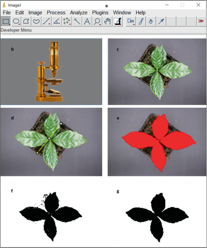

  

  Schematic representation of the steps taken to analyse images using ImageJ. a ImageJ software menu bar. b ImageJ software logo. c A picture of the seedling to be imported to the software for analysis. d Calibration line drawn from the internal diameter (100 mm) of the pot. e Red pixels adjusted using sliders to cover the seedling. f Output of the first image analysis with noise. g Output after noise removal

• 3. Download and install ImageJ software on your computer (laptop or desktop) (Fig. 7b).

• 4. Choose between Windows or Mac depending on the operating system of your device (https://imagej.nih.gov/ij/download.html).

• 5. Open the software on your device to display the menu bar (Fig. 7a).

• 6. Import your image (png) into the software (File→Open→Select image) (Fig. 7c).

• 7. Calibrate your analysis by using the line tool to draw an imaginary line of the known distance, for instance internal diameter of the pot (60 mm) (Fig. 7d).

• 8. Set the scale for your analysis (Image→Set scale→Known distance→measured units e.g., cm or mm).

• 9. Adjust sliders to fully select the plant in the image (Image→Adjust→Colour threshold). Select red colour for the pixels (Fig. 7e).

• 10. Just before analysis, set parameters of interest (Analyse→Set measurement→Area, perimeter, etc.).

• 11. Invert the image output to black and white in the masks (Image→lookup tables→Invert LUT).

• 12. Perform image analysis to estimate area of spread (Analyse→Particles→Show masks→Display clear results→OK) (Fig. 7f).

• 13. Remove the noise from the mask (Process→Binary→Erode or Dilate) to generate an output image that is more similar to the input image (Fig. 7g).

• 14. Finally, repeat the analysis of particles (step 12) to obtain the measurement of the preferred parameter in the set units, for instance the area in square mm (mm²) or perimeter (mm).

• 15. The data can be entered in the Field Book for the respective trait.

3.4 Statistical Analysis

• 1. Acquire the data from Field Book, or any other electronic data storage device.

• 2. Ensure internet connection on your Android device with the application containing data.

• 3. Export the data to your storage place (Fig. 2h, i).

• 4. Retrieve the data (Excel file, “csv” format) from the destination storage.

• 5. Save the latest Excel data file on your computer for statistical analysis. The file contains all the data from the entire data collection procedure.

• 6. Alternatively, connect the Android device to a computer with a USB cable, copy the data file directly from the export folder in the Field Book application.

• 7. Use any statistical software familiar to you to determine phenotypic variability within your population.

• 8. For every trait measured, calculate the average per treatment.

• 9. Perform pairwise comparisons for every mutagen treatment and non-treated control to determine an increase or reduction in the measured trait.

• 10. Likewise, perform multiple comparison analysis of every trait to determine whether phenotypic variation exists in the mutant population.

• 11. Explore the distribution of your data points per treatment. Pay attention to outliers, they could be of potential interest, for instance, high yielding.

• 12. If necessary, compute percentage increase or reduction in the trait with reference to control.

• 13. Determine levels of statistical significance (p ≤ 0.05) between or among treatments.

• 14. The outputs can be represented graphically (Fig. 8) or in tabular formats.

  Fig. 8

  

  Example data demonstrating the induced phenotypic variability in the coffee M₁ population treated with  different doses of EMS (%EMS) and gamma-rays (gray—Gy). a Plant height measured three years after planting. b Leaf length measured from the petiole to the apex. c Leaf width measured at the widest part of the leaf. d Estimated Leaf Area (ELA) based on leaf length and leaf width measurements using allometric model, ELA = 0.99927*(L*(– 0.14757 + 0.60986*W)) according to Unigarro-Muñoz et al. (2015)

3.5 Establishment of M₂ Population

• 1. To establish the M₂ population, harvest M₁ berries from each primary branch of each M₁ plant (see Note 8).

• 2. Mature berries can be sown/planted immediately after harvesting and depulping or kept for a period less than three months.

• 3. Prepare labels with all the necessary information including treatment, mother plant, date etc.

• 4. Remove the pulp from the berries.

• 5. Plant the beans in the previously prepared pots (see Note 8).

• 6. After sowing, water the pots periodically before and after emergence of the seedlings.

• 7. Record the number of days to emergence or germination.

• 8. At six months after sowing, the seedling will be ready for transplanting to 5 L pots.

• 9. Maintain M₂ plants following the procedures described in Sect. 3.1.

• 10. Collect data using the electronic phenotyping tools described in Sect. 3.2.1.

• 11. Monitor seedlings/plants for unique phenotypes (Fig. 4).

• 12. Prior to transplanting, take aerial images of the seedlings to determine the area of the seedlings canopies.

• 13. During plant growth, measure or score and record the growth traits as described in Sect. 3.2.2.

• 14. Measure and record yield traits as described in Sect. 3.2.3.

• 15. Assess the population for other traits including quality, resistance or tolerance to major pests and diseases, drought and other abiotic stresses (see Note 9).

• 16. Acquire data from the images using ImageJ as described in Fig. 7.

• 17. Likewise, export data from Field Book following procedures described in Fig. 2.

• 18. Analyse data using appropriate statistical analysis tools.

4 Notes

• 1. M₁ coffee seedlings were derived from C. arabica var. Venecia seed following EMS and gamma-ray mutagenesis (see Chap. “Chemical Mutagenesis of Mature Seed of Coffea arabica L. var. Venecia Using EMS”). The seeds were subjected to different doses of the respective mutagens after performing a chemotoxicity or radiosensitivity test.

• 2. Ensure that seedlings are transplanted with soil attached for optimal growth. Watering the seedlings one day before transplanting is recommended. The 5 L pots hold sufficient soil to support plant growth for at least three reproductive cycles under good management.

• 3. A completely randomised experimental design (CRD) is chosen since the experiment is set up in the greenhouse. The assumption is that a greenhouse provides a homogeneous micro-environment. The 100 cm space between blocks enables convenient working space during experimental management, data collection, etc.

• 4. Nutrients are important for plant growth and development. Some effects of induced mutagenesis are similar to those caused by nutrient deficiencies, such as chlorosis (yellowing, mosaics) and stunted growth. Therefore, apply complex fertilisers to support optimal plant growth and to have good and valid data on the mutant population. At transplanting, mixing fertilisers with the potting medium may not be necessary since the medium is still fresh. However, replenishing nutrients at three months intervals using nitrogen, phosphate and potassium (NPK) improves root and vegetative growth.

• 5. Pest and disease outbreaks in the mutant population should be prevented. Frequent monitoring of the plants is necessary. Like nutrient deficiencies, pests and disease symptoms can be similar to those resulting from mutations, such as chlorophyl aberrations, the curling of leaves and stunted growth. In case of any outbreaks, apply broad-spectrum systemic chemicals to provide an effective control strategy to diverse pests and diseases. Moreover, some insect pests attack the lower leaf surfaces or stems inside the canopy; hence, the pests will not be reached by contact pesticides administered by spraying. Systemic pesticides have less harmful effects on the natural biological agents such as ladybugs, wasps and ants as opposed to contact pesticides. For human safety reasons, follow the standard precautionary procedures for handling agricultural chemicals.

• 6. Field Book is an Android, open-access application that can be downloaded from the Google Play Store onto Android phones and tablets (https://github.com/PhenoApps/Field-Book). Using the application does not require connection to the internet. Prior to use, design your experimental layout in Excel on your computer. Connect your Android device to the computer, copy the Excel file and paste it into the import folder of the Fieldbook application. Finally, import the Excel file as a field in the application. Add your traits of interest in the application and define them as numerical, categorical, text, percentage, date, etc. After successful addition of the traits, data collection can start immediately. After completing data collection, it can be exported to a preferred data storage centre such as the cloud, Dropbox or shared via E-mail and Bluetooth, among others.

• 7. Measuring plant height is important to monitor differences in growth rate and identify dwarf or tall phenotypes in the mutant population.

• 8. Harvest berries from individual M₁ plants. Depending on the objective of the study, the position of the M₂ berries on individual M₁ plants can be mapped by recording the number and position of the branch and node for every harvested berry. Plant the beans in the previously prepared pots following the pre-determined method, for instance, bulk method or single seed descent (FAO/IAEA 2018).

• 9. In most cases, the goal of a mutation breeding program is to improve one particular trait. However, one can simultaneously screen the mutant population for other traits of interest including quality, resistance or tolerance to major pests and diseases, drought, etc.

References

Carvalho A, Medina Filho HP, Fazuoli LC, Guerreiro Filho O, Lima MMA (1991) Aspectos genéticos do cafeeiro. Revista Brasileira de Genética l4:135–183
FAO (2015) Food and agriculture organisation, FAO statistical pocketbook. ISBN 978-108894-4
FAO/IAEA (2018) Manual on mutation breeding, 3rd edn. In: Spencer-Lopes MM, Forster BP, Jankuloski L (eds) Food and agriculture organization of the united nations. Rome, Italy, 301 p
Hartmann A, Czauderna T, Hoffmann R, Stein N, Schreiber F (2011) HTPheno: an image analysis pipeline for high-throughput plant phenotyping. BMC Bioinformatics 12(1):1–9
IPGRI (1996) Descriptors for Coffee (Coffea Spp. and Psilanthus Spp.). International Plant Genetic Resources Institute, Bioversity International p 36.
Jain MS (2005) Major mutation-assisted plant breeding programs supported by FAO/IAEA. Plant Cell Tissue Organ Cult 82:113–123
Lashermes P, Trouslot P, Anthony F, Combes MC, Charrier A (1996) Genetic diversity for RAPD markers between cultivated and wild accessions of Coffea arabica. Euphytica 87:59–64
Lashermes P, Bertrand B, Etienne H (2009) Breeding coffee (Coffea arabica) for sustainable production. In: Mohan JS, Priyadarshan PM (eds) Breeding plantation tree crops: tropical species. Springer, New York, pp 525–543. https://doi.org/10.1007/978-0-387-71201-7_14
Mechael PN (2009) The case for mHealth in developing countries. Innov Technol Gov Globalization 4(1):103–118
Ouma T, Kavoo A, Wainaina C, Ogunya B, Karanja M, Kumar PL, Shah T (2019) Open data kit (ODK) in crop farming: mobile data collection for seed yam tracking in Ibadan, Nigeria. J Crop Improv 33(5):605–619. https://doi.org/10.1080/15427528.2019.1643812
Pathirana R, Vitiyala T, Gunaratne NS (2009) Use of induced mutations to adopt aromatic rice to low country conditions of Sri Lanka. In: Induced plant mutations in the genomics era. Proceedings of an international joint FAO/IAEA symposium. International atomic energy agency, Vienna, Austria, 2009, pp 388–390
Pathirana R (2011) Plant mutation breeding in agriculture. Perspectives in agriculture, veterinary science, nutrition and natural resources. CAB International 2011 6, No 032
Prasad P, Agbona A, Kulakow P, Rabbi I, Egesi C, Parkes E, Mueller L (2018) Cassavabase, an advantage for IITA cassava breeding program. In: 4th International Cassava conference poster session presented at: the GCP21, at Cotonou Benin June 11–15; Cotonou, Benin
Rife TW, Poland JA (2014) Field book: an open-source application for field data collection on android. Crop Sci 54. https://doi.org/10.2135/cropsci2013.08.0579
Sabina L (2022) How data cross borders: globalizing plant knowledge through transnational data management and its epistemic economy. In: Krige J (ed) Knowledge flows in a global age: a transnational approach. University of Chicago Press, Chicago, pp 305–332. https://doi.org/10.7208/chicago/9780226820378-011
Schindelin J, Arganda-Carreras I, Frise E, Kaynig V, Longair M, Pietzsch T, Cardona A (2012) Fiji: an open-source platform for biological-image analysis. Nat Methods 9(7):676–682
Singh MK, Chetia S, Singh M (2017) Detection and classification of plant leaf diseases in image processing using MATLAB. Int J Life Sci Res 5(4):120–124
Ulukapi K, Nasircilar AG (2018) Induced mutation: creating genetic diversity in plants. In: Genetic diversity in plant species-characterization and conservation. IntechOpen
Unigarro-Muñoz CA, Hernández-Arredondo JD, Montoya-Restrepo EC, Medina-Rivera RD, Ibarra-Ruales LN, CarmonaGonzález CY, Flórez-Ramos CP (2015) Estimation of leaf area in coffee leaves (Coffea arabica L.) of the Castillo® variety. Bragantia 74:412–416. https://doi.org/10.1590/1678-4499.0026
Acknowledgements
The authors wish to thank the International Atomic Energy Agency and the Government of Belgium for their financial support through the CRP D22005 ‘Efficient Screening Techniques to Identify Mutants with Disease Resistance for Coffee and Banana’ and the Peaceful Use Initiative project ‘Enhancing Climate Change Adaptation and Disease Resilience in Banana-Coffee Cropping Systems in East Africa’, respectively.
Author information
Authors and Affiliations
Corresponding authors
Editor information
Editors and Affiliations
Rights and permissions
Open Access This chapter is licensed under the terms of the Creative Commons Attribution 4.0 International License (http://creativecommons.org/licenses/by/4.0/), which permits use, sharing, adaptation, distribution and reproduction in any medium or format, as long as you give appropriate credit to the original author(s) and the source, provide a link to the Creative Commons license and indicate if changes were made.
The images or other third party material in this chapter are included in the chapter's Creative Commons license, unless indicated otherwise in a credit line to the material. If material is not included in the chapter's Creative Commons license and your intended use is not permitted by statutory regulation or exceeds the permitted use, you will need to obtain permission directly from the copyright holder.
Copyright information
© 2023 The Author(s)
About this chapter
Cite this chapter
Nkurunziza, R., Jankowicz-Cieslak, J., Werbrouck, S.P.O., Ingelbrecht, I.L.W. (2023). Use of Open-Source Tools for Imaging and Recording Phenotypic Traits of a Coffee (Coffea arabica L.) Mutant Population. In: Ingelbrecht, I.L., Silva, M.d.C.L.d., Jankowicz-Cieslak, J. (eds) Mutation Breeding in Coffee with Special Reference to Leaf Rust. Springer, Berlin, Heidelberg. https://doi.org/10.1007/978-3-662-67273-0_14
Download citation
DOI: https://doi.org/10.1007/978-3-662-67273-0_14
Published:
Publisher Name: Springer, Berlin, Heidelberg
Print ISBN: 978-3-662-67272-3
Online ISBN: 978-3-662-67273-0
eBook Packages: Biomedical and Life SciencesBiomedical and Life Sciences (R0)