
Abstract
The first step towards an effective field theory for spontaneously broken spacetime symmetry is the construction of the nonlinear realization of the symmetry. This chapter develops the theory of nonlinear realizations of spacetime symmetries in close parallel with the previous discussion of internal symmetry. There are however some important differences. Notably, the spacetime coordinates and fields have to be treated together as independent variables, spanning a larger manifold on which the symmetry acts. The points of this manifold are no longer in a one-to-one correspondence with possible values of the order parameter. Likewise, the isotropy group of any point no longer corresponds to the subgroup, left unbroken in the ground state. These obstacles can be bypassed by focusing on the subgroup of symmetries that fix a given spacetime point. This leads to an unambiguous identification of the independent Nambu–Goldstone degrees of freedom, and allows for a straightforward generalization of the standard nonlinear realization of internal symmetry. The conditions under which such standard nonlinear realization of spacetime symmetries is exhaustive are discussed explicitly. Finally, several illustrative examples are worked out in detail.
You have full access to this open access chapter, Download chapter PDF
In Part III of the book, I assumed that whatever the full symmetry of the system, only internal symmetry is spontaneously broken. Moreover, I only considered two possibilities for the symmetry of the underlying spacetime. For nonrelativistic systems, I assumed invariance under spacetime translations and spatial rotations; this symmetry is sometimes called Aristotelian. In case of relativistic systems, the Aristotelian symmetry is turned into Poincaré symmetry by adding invariance under Lorentz boosts. Both of these spacetime symmetries are easy to implement provided they are not spontaneously broken. Invariance under spacetime translations is ensured by demanding that the Lagrangian density of the theory does not depend explicitly on spacetime coordinates. Invariance under spatial or spacetime rotations can be guaranteed by contracting indices appropriately using ordinary tensor calculus.
The situation becomes subtle when the spacetime symmetry is spontaneously broken, or when a different spacetime symmetry than Poincaré or Aristotelian is present. It is known that there are in fact multiple mathematically consistent kinematical groups including spacetime translations, spatial rotations and boosts [1]. Here I will consider in particular the Galilei symmetry, relevant for effective field theories (EFTs) of many nonrelativistic systems. Due to the mathematical structure of the Galilei group, the theory of its representations, and thus construction of Galilei-invariant actions, is highly nontrivial. For an overview of other possible non-Lorentzian kinematics and the associated spacetime geometry, see [2].
The EFT for broken spacetime symmetries finds natural application in cosmology. To make the methodology developed below useful also there, I will make an exception and initially allow for theories defined on a generic spacetime manifold. Some simplifying assumptions on the spacetime manifold will be necessary, but will only be introduced when needed. Otherwise, the general philosophy of construction of EFTs for spontaneously broken spacetime symmetry is the same as in Part III. I will start in this chapter by classifying possible nonlinear realizations of spacetime symmetry. In Chaps. 13 and 14, I will then utilize the results to build effective actions. Unfortunately, there are no general explicit expressions for effective Lagrangians akin to those for internal symmetries, worked out in Chap. 8. I will therefore have to resort to outlining the basic algorithm and working out some illustrative examples.
1 Reminder of Nonlinear Realization of Internal Symmetry
The material of this chapter closely parallels Chap. 7, which the reader is advised to remind themselves of before proceeding further. In order to underline the basic logic, let me however give at least a brief summary of the steps we took in Chap. 7.
We used the fact that internal symmetries in the sense of Sect. 4.1.1 are point transformations that only act on fields and leave spacetime coordinates intact. This allows for a geometric reformulation of the problem of classifying all nonlinear realizations of internal symmetry. Namely, if the fields take values from a manifold \(\mathcal {M}\), then realizing the internal symmetry group G on them amounts to defining an action of G on \(\mathcal {M}\). While the action of the symmetry group is assumed to exist globally on the whole manifold \(\mathcal {M}\), its explicit expression requires a set of local coordinates. Thus, all statements depending on a specific choice of coordinates are without further qualification valid only in a local coordinate patch.
We start by picking a point \(\psi _0\in \mathcal {M}\).Footnote 1 The subgroup \(H_{\psi _0}\) of elements of G that map \(\psi _0\) to itself is called its isotropy group. Whenever \(H_{\psi _0}\) is compact, there are local coordinates \((\pi ^a,\chi ^\varrho )\) on \(\mathcal {M}\) such that \(\psi _0\) corresponds to \(\pi ^a=\chi ^\varrho =0\) , and \(H_{\psi _0}\) acts separately and linearly on \(\pi ^a\) and \(\chi ^\varrho \). Moreover, the set of points \((\pi ^a,0)\) spans a submanifold of \(\mathcal {M}\), equivalent to the coset space \(G/H_{\psi _0}\). This makes it possible to encode \(\pi ^a\) in a unique representative element \(U(\pi )\) of the corresponding left coset of \(H_{\psi _0}\) in G. The representative element can be chosen so that the point \(\psi _0\) is mapped to \(U(0)=e\). In addition, the linear representation of the isotropy group \(H_{\psi _0}\) on \(\pi ^a\) is realized by the adjoint action, \(U(\pi )\to hU(\pi )h^{-1}\), \(h\in H_{\psi _0}\). Altogether, the action of G on \(\mathcal {M}\) in the standard coordinates \((\pi ^a,\chi ^\varrho )\) is fixed by the choice of representative \(U(\pi )\) and of the linear representation of \(H_{\psi _0}\) on \(\chi ^\varrho \).
In physics terms, every point \(\psi _0\in \mathcal {M}\) defines a specific value of the order parameter for spontaneous symmetry breaking (SSB). The isotropy group \(H_{\psi _0}\) corresponds to the unbroken subgroup of G. Once treated as maps from the spacetime to \(\mathcal {M}\), \(\pi ^a\) become the Nambu–Goldstone (NG) fields implied by SSB, whereas \(\chi ^\varrho \) are usually called matter fields. The same symmetry-breaking pattern \(G\to H\) may be realized by different order parameters, and thus on different target manifolds \(\mathcal {M}\). This however only affects the number and type of matter fields present. The NG fields are identified unambiguously as coordinates on the coset space \(G/H\), and are in a one-to-one correspondence with the generators of broken symmetry.
Moving now to spacetime symmetries, we will be able to follow the mathematical construction of nonlinear realization of internal symmetry very closely. We will only have to introduce one important modification, taking into account the distinction between fields and coordinates. However, the mapping to the physical concepts of SSB and NG bosons will turn out to be much more intricate.
2 Spacetime Symmetry as a Point Transformation
Consider a theory of a set of bosonic fields \(\psi ^i\) living on a D-dimensional spacetime manifold M. It is temporarily convenient to treat \(\psi ^i\) and the spacetime coordinates \(x^\mu \) on equal footing as independent variables spanning the product manifold \(\mathcal {M}\times M\). This allows us to view the action of a spacetime symmetry (in the sense of Sect. 4.1.1) as a special case of a point transformation on \(\mathcal {M}\times M\). See Fig. 12.1 for a visualization. Formally, the action of a spacetime symmetry group G on \(\mathcal {M}\times M\) constitutes a set of maps \(T_g\), or equivalently functions \(\mathbb {F}^i\) and \(\mathbb {X}^\mu \), such that
The functions \(\mathbb {F}^i\) and \(\mathbb {X}^\mu \) cannot be chosen arbitrarily, but have to respect the structure of G. First, the unit element \(e\in G\) must be realized by an identity transformation,

Visualization of the action of a spacetime symmetry on the product manifold \(\mathcal {M}\times M\). The transformation of the spacetime coordinates \(x^\mu \) is independent of the fields \(\psi ^i\). For fixed \(x_0\in M\) and \(g\in G\), the symmetry thus acts as a map between the slices \(\mathcal {M}\times \{x_0\}\) and \(\mathcal {M}\times \{ \mathbb {X}(x_0,g)\}\), indicated by the dashed lines
Second, the group multiplication law dictates that for any \(g_1,g_2\in G\),
Finally, for any \(g\in G\) the map \(T_{g^{-1}}\) must be the inverse of \(T_g\),
The special case of (12.1) where \(\psi ^{\prime i}=\mathbb {F}^i(\psi ,g)\) and \(\mathbb {X}^\mu (x,g)=x^\mu \) corresponds to an internal symmetry.Footnote 2 Another special case is a purely spacetime transformation, where \(\mathbb {F}^i(\psi ,x,g)=\psi ^i\) for all \(\psi \in \mathcal {M}\) and \(x\in M\). It follows from the conditions on the functions \(\mathbb {X}^\mu \) in (12.2)–(12.4) that purely spacetime transformations form a subgroup of the symmetry group G. Here I will make a technical assumption that will prove essential for setting up standard coordinates on the product manifold \(\mathcal {M}\times M\). Namely, I will assume that the subgroup of G of purely spacetime transformations acts transitively on every slice \(\{\psi \}\times M\) with fixed \(\psi \in \mathcal {M}\). Loosely speaking, this requires that the spacetime manifold M has sufficient symmetry that turns it into a homogeneous space. Now choose an arbitrary \(x_0\in M\) and keep it fixed. By our assumption, for any \(x\in M\) there is a purely spacetime transformation \({\mathcal T_{{x_0}\to {x}}}\in G\) that maps \(x_0\) to x. Typically, there will be multiple such transformations; we then have to choose one \({\mathcal T_{{x_0}\to {x}}}\) by convention. For flat spacetimes, it is natural to use a translation connecting the two points. However, we do not have to be that specific at this stage, keeping in mind that M may be curved.
Eventually, we would like to treat \(\psi ^i\) as functions on the spacetime. Mathematically, this amounts to replacing the action of the symmetry group G on \(\mathcal {M}\times M\) with one on maps \(M\to \mathcal {M}\). Such an induced action is easy to write down thanks to the assumption that the transformation of the coordinates is independent of the fields. Thus, the fields \(\psi ^i(x)\) are mapped to \(\psi ^{\prime i}(x,g)\) such that
for any \(g\in G\). We will need (12.5) once we want to construct a G-invariant effective action for the fields. For the time being, however, I will pursue the analogy with Chap. 7 and focus on the action of G on the product manifold \(\mathcal {M}\times M\).
3 Standard Nonlinear Realization
For every point \((\psi ,x)\in \mathcal {M}\times M\) there is an isotropy group consisting of elements of G that map the point to itself,
The setup of nonlinear realization of internal symmetry as reviewed in Sect. 12.1 would naively suggest that we now choose a point \((\psi _0,x_0)\in \mathcal {M}\times M\). In its neighborhood, we could then establish the standard nonlinear realization of G in the usual manner. There are however two problems with this naive approach. First, we eventually want to treat fields as functions, defined globally on the whole spacetime M, as long as global coordinates on M exist. Second, the fields should be functions of the original, physical coordinates \(x^\mu \), not of some new variables whose dependence on \(\psi ^i\) and \(x^\mu \) is beyond our control.
In order to reach these goals, we take an intermediate step, introducing an isotropy group of a chosen spacetime point,
Obviously, \(H_{(\psi ,x)}\) is a subgroup of \(H_x\) for any \(\psi \in \mathcal {M}\). Moreover, having fixed a reference point \(x_0\in M\), we can use the maps \({\mathcal T_{{x_0}\to {x}}}\) to show that, in analogy with (7.7), isotropy groups at different spacetime points are related by conjugation,
Example 12.1
Let \(\psi \) be a complex Schrödinger field so that \(\mathcal {M}\simeq \mathbb {C}\), and let M be the flat Galilei spacetime. The action (11.43) of a Galilei boost with velocity \(\boldsymbol v\) corresponds to

We assume that in addition to boosts, the symmetry group G also includes spacetime translations, spatial rotations, and the internal \(\mathrm {U}(1)\) symmetry of phase transformations. For \(x_0^\mu =(\boldsymbol x_0,t_0)=(\boldsymbol 0,0)\), we find \(H_{x_0}\simeq [\mathrm {SO}(d)\ltimes \mathbb {R}^d]\times \mathrm {U}(1)\), consisting of spatial rotations, Galilei boosts, and the phase transformations. In the special case of \(\psi _0=0\), \(H_{(\psi _0,x_0)}\simeq H_{x_0}\). Otherwise, for any \(\psi _0\neq 0\), \(H_{(\psi _0,x_0)}\simeq \mathrm {SO}(d)\ltimes \mathbb {R}^d\subsetneq H_{x_0}\). The isotropy groups for other spacetime points are obtained by conjugation (12.8) using the spacetime translation \({\mathcal T_{{x_0}\to {x}}}(\psi ,\boldsymbol x',t')\equiv (\psi ,\boldsymbol x'+\boldsymbol x-\boldsymbol x_0,t'+t-t_0)\).Footnote 3
For any fixed \(x\in M\), the transformation of \((\psi ^i,x^\mu )\) under \(g\in H_x\) is determined by the functions \(\mathbb {F}^i(\psi ,x,g)\). In other words, these functions define an action of \(H_x\) on the slice \(\mathcal {M}\times \{x\}\simeq \mathcal {M}\). This makes it possible, following now Chap. 7 verbatim, to introduce a standard set of field coordinates on \(\mathcal {M}\). Together with the spacetime coordinates \(x^\mu \), this defines a parameterization of the whole manifold \(\mathcal {M}\times M\), in which the action of G takes a standard form. In order to keep the main results of this chapter together in one place, I will first give a concise overview of the ensuing standard realization of spacetime symmetry. Afterwards, I will stress some of its subtleties. A number of examples is worked out in detail in Sect. 12.4; the reader may want to consult these alongside the formal construction developed below.
3.1 Summary of the Construction
Consider the action of a continuous group G on the product manifold \(\mathcal {M}\times M\) via a set of point transformations of the type (12.1). It is assumed that G includes a set of purely spacetime transformations that act transitively on every slice \(\{\psi \}\times M\) with fixed \(\psi \in \mathcal {M}\). I will for simplicity choose the reference point \(x_0\in M\) with \(x^\mu _0=0\) and denote as \(\mathcal {T}_{x}\equiv {\mathcal T_{{0}\to {x}}}\) the purely spacetime transformation that maps \(x_0\) to \(x\in M\).
The slice \(\mathcal {M}\times \{0\}\simeq \mathcal {M}\) carries an action of the isotropy group \(H_0\). Choose a fixed point \(\psi _0\in \mathcal {M}\). Assuming that the isotropy subgroup \(H_{(\psi _0,0)}\) is compact, it is always possible to find coordinates \((\pi ^a,\chi ^\varrho )\) on \(\mathcal {M}\times \{0\}\) with the following properties:
-
The point \(\psi _0\) corresponds to \((\pi ^a,\chi ^\varrho )=(0,0)\). Also, the set of points \(\{(\pi ^a,0)\}\) spans a submanifold of \(\mathcal {M}\times \{0\}\), equivalent to the coset space \(H_0/H_{(\psi _0,0)}\).
-
The coordinates \(\pi ^a\) parameterize uniquely a representative \(U(\pi )\in H_0\) of the corresponding left coset of \(H_{(\psi _0,0)}\) in \(H_0\) such that \(U(0)=e\).
-
The subgroup \(H_{(\psi _0,0)}\) acts on \(H_0/H_{(\psi _0,0)}\) by adjoint action, \(U(\pi )\to hU(\pi )h^{-1}\) with \(h\in H_{(\psi _0,0)}\), which induces a linear transformation of the coordinates \(\pi ^a\).
-
The whole group \(H_0\) acts on \(\mathcal {M}\times \{0\}\) by left multiplication as
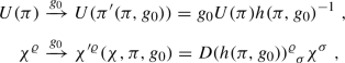 (12.10)
where \(g_0\in H_0\) and \(h(\pi ,g_0)\in H_{(\psi _0,0)}\). Moreover, \(D(h)\) is a matrix representation of \(H_{(\psi _0,0)}\). Altogether, the action of \(H_0\) on \(\mathcal {M}\times \{0\}\) is fixed by the choice of representation D of \(H_{(\psi _0,0)}\) and the choice of parameterization \(U(\pi )\) of the coset space \(H_0/H_{(\psi _0,0)}\).

This finishes the setup of coordinates and the action of \(H_0\) on the domain \(\Omega _{\psi _0}\times \{0\}\); \(\Omega _{\psi _0}\) is a neighborhood of \(\psi _0\) in \(\mathcal {M}\) where the coordinates \((\pi ^a,\chi ^\varrho )\) are well-defined. As the next step, we transport the coordinates \((\pi ^a,\chi ^\varrho )\) to the whole spacetime using the maps \(\mathcal {T}_{x}\). This leads to coordinates \((\pi ^a,\chi ^\varrho ,x^\mu )\) on the domain \(\Omega _{\psi _0}\times M\) (see Fig. 12.2). Intuitively, we require that all points of the slice \(\{\psi \}\times M\) with fixed \(\psi \in \Omega _{\psi _0}\) have the same coordinates \(\pi ^a,\chi ^\varrho \). Technically, we set
By (12.8), this fixes the action of the isotropy group \(H_x\) on \(\mathcal {M}\times \{x\}\). Indeed, for any \(g_x\in H_x\) there is a unique \(g_0\in H_0\) such that \(g_x=\mathcal {T}_xg_0\mathcal {T}_x^{-1}\). This leads to
Moreover, (12.8) guarantees that for any \(g_x\in H_{(\psi _0,x)}\), \(g_0\in H_{(\psi _0,0)}\). Therefore, the isotropy subgroup \(H_{(\psi _0,x)}\) is realized on the slice \(\mathcal {M}\times \{x\}\) by linear transformations of \(\pi ^a\) and \(\chi ^\varrho \) for any \(x\in M\).

Schematic visualization of the domain (shaded area) on the manifold \(\mathcal {M}\times M\) where the standard coordinates \((\pi ^a,\chi ^\varrho ,x^\mu )\) are well-defined. The domain \(\Omega _{\psi _0}\subset \mathcal {M}\) carries a local coordinate patch with the field variables \((\pi ^a,\chi ^\varrho )\)
The structure we already have extends uniquely to an action of the entire group G on the entire manifold \(\mathcal {M}\times M\), or at least on \(\Omega _{\psi _0}\times M\). Namely, note that the action of any \(g\in G\) on a chosen point \((\psi ,x)\) can be composed of the action of an element of \(H_x\) and a purely spacetime transformation, see Fig. 12.3. Indeed, decompose
with the shorthand notation  . The group element \(g_x(x,g)\) maps \((\psi ^i,x^\mu )\) to \((\mathbb {F}^i(\psi ,x,g),x^\mu )\) for any \(\psi \in \mathcal {M}\) and thus belongs to \(H_x\). It corresponds to an element \(g_0(x,g)\in H_0\) by
  . Together with (12.12), this leads to the final expression for the action of G within \(\Omega _{\psi _0}\times M\),
This completes the setup of the nonlinear realization of G. I assumed an a priori knowledge of the transformation properties of the spacetime coordinates, that is the functions \(\mathbb {X}^\mu (x,g)\). With this provision, the action of G is uniquely fixed by the structure of the isotropy groups \(H_0\) and \(H_{(\psi _0,0)}\), and by the representation \(D(h)\) of \(H_{(\psi _0,0)}\). In the process, we made some choices, including the choice of the representative \(U(\pi )\) parameterized by \(\pi ^a\) and of the element \(\mathcal {T}_x\in G\) representing a spacetime point \(x\in M\). These are just two sides of the same coin, pertinent respectively to the manifolds \(\mathcal {M}\) and M.

For any fixed point \((\psi ,x)\in \mathcal {M}\times M\), the action of a chosen element \(g\in G\) can be composed from actions of an element of \(H_x\) and a purely spacetime transformation
Complicated as it might seem, (12.14) actually encodes in a rather simple manner the action of G by left matrix multiplication. Indeed, let us represent the point \((\pi ^a,\chi ^\varrho ,x^\mu )\) formally by \(\mathcal {T}_x(U(\pi ),\chi ^\varrho )\). Then left multiplication by any \(g\in G\) gives

which exactly copies (12.14) in the matrix notation of (12.10). This shows that it is not actually necessary to decompose every \(g\in G\) into a product of an element of \(H_x\) and a purely spacetime transformation as in (12.13). It is sufficient to observe that for any \(x\in M\) and \(g\in G\),  fixes the origin of M and thus belongs to \(H_0\).
3.2 Relation to Physics of Broken Spacetime Symmetry
Mathematically, the generalization of the standard nonlinear realization from internal to spacetime symmetry was relatively straightforward, perhaps even deceivingly so. A number of its features thus deserve pointing out before we proceed to examples.
Universality of the Construction
In Chap. 7 we found out that provided the isotropy group H is compact, the standard nonlinear realization captures all possible actions of the symmetry group G. Furthermore, I remarked that even if H is noncompact, the construction still goes through, but is no longer guaranteed to be exhaustive, provided the coset space \(G/H\) is reductive. The same applies here with the necessary modifications. The universality of the standard nonlinear realization is ensured if \(H_{(\psi _0,0)}\) is compact. Even if it is not, the construction is still consistent, yet not necessarily exhaustive, if the coset space \(H_0/H_{(\psi _0,0)}\) is reductive. Reference [3] gives an explicit example of a group action that cannot be obtained from the standard nonlinear realization. There \(G\simeq \mathrm {SO}(2,1)\) acts on \(\mathcal {M}\simeq \mathbb {R}\), the isotropy subgroup being the noncompact affine group \(\mathrm {Aff}(1)\simeq \mathbb {R}^+\ltimes \mathbb {R}\).
A possible point of concern might be that I assumed an a priori knowledge of the action of G on spacetime coordinates. This is however not a source of any hidden ambiguity. For one thing, the action of symmetry on spacetime coordinates is usually known. It is the classification of NG fields and their transformation properties that we are after. Moreover, even if unknown a priori, the functions \(\mathbb {X}^\mu (x,g)\) can be constrained following the same philosophy. Namely, restricting (12.1) to the coordinates \(x^\mu \) gives a group of well-defined transformations on M. If desired, possible forms of these transformations can be classified using the setup of Chap. 7.
Fate of Descendant Symmetries
Recall the discussion of locally equivalent symmetries in Sect. 11.1. As explained therein, one can assume without loss of generality that the functions  vanish at the origin, \(x^\mu =0\). Provided the localized parent transformation in (11.1) does not involve any derivatives of \(\epsilon ^A_1(x)\), the action of the descendant symmetry at the origin vanishes. In the standard nonlinear realization, such a descendant symmetry therefore automatically belongs to \(H_{(\psi _0,0)}\) and does not give rise to any NG variables \(\pi ^a\).
Physical Unbroken Symmetry
In contrast to the internal symmetry case, a single point \((\psi ,x)\in \mathcal {M}\times M\) cannot unambiguously represent the order parameter for SSB. The order parameter rather corresponds to a function \(\varphi ^i:M\to \mathcal {M}\). A particular value of the order parameter then defines a submanifold, \(\mathcal {M}_\varphi \equiv \{(\varphi ^i(x),x^\mu )\,\vert \,x\in M\}\subset \mathcal {M}\times M\). Accordingly, neither \(H_x\) nor \(H_{(\varphi (x),x)}\) can be identified with the subgroup of unbroken symmetries, \(H_\varphi \). The latter rather consists of all elements of G that preserve the manifold \(\mathcal {M}_\varphi \), that is map points on \(\mathcal {M}_\varphi \) to other points on \(\mathcal {M}_\varphi \). With the help of (12.5), this translates to the condition \(\varphi ^i(\mathbb {X}(x,g))=\mathbb {F}^i(\varphi (x),x,g)\) for all \(x\in M\). This constraint is highly implicit; in practice it is usually much easier to check its infinitesimal form,
The functions \(F^i_A\) and \(X^\mu _A\) define the action of the generator \(Q_A\) of G. The reconstruction of the group \(H_\varphi \) from the solutions to (12.16) is based on the correspondence between a Lie group and its Lie algebra. An example of a possible pitfall this approach may fall into, in the context of isometries of a Riemannian manifold, is given in Appendix A.6.2.
Example 12.2
Suppose that the order parameter is constant, \(\varphi ^i(x)\equiv \varphi ^i_0\). It follows that the “vacuum submanifold” is \(\mathcal {M}_\varphi =\{\varphi _0\}\times M\). According to (12.1), the unbroken subgroup is
Any purely spacetime symmetry automatically belongs to \(H_{\varphi _0}\). In other words, purely spacetime symmetries can only be broken by a coordinate-dependent order parameter. On the other hand, for internal symmetries, the condition in (12.17) reduces to \(\mathbb {F}^i(\varphi _0,g)=\varphi ^i_0\). Since internal symmetries by construction do not affect the coordinates \(x^\mu \), the definitions of \(H_{(\varphi _0,x)}\) and \(H_{\varphi _0}\) in this special case coincide. At the same time, for internal symmetries we have trivially \(H_x\simeq G\) for any \(x\in M\), hence \(H_x/H_{(\varphi _0,x)}\simeq G/H_{\varphi _0}\). This verifies that for internal symmetries, the more general formalism developed here boils down to that of Chap. 7.
Classification of Order Parameter Fluctuations
For internal symmetries, independent fluctuations of the order parameter are in a one-to-one correspondence with the NG fields \(\pi ^a\). It would therefore be tempting to conclude that in the more general case of spacetime symmetries, they are classified by the coset space \(H_0/H_{(\psi _0,0)}\). The latter however only counts the NG variables \(\pi ^a\), realizing nonlinearly the action of \(H_0\). Our parameterization (12.11) of the manifold \(\mathcal {M}\times M\) also involves the action of the “translations” \(\mathcal {T}_x\). Being purely spacetime, these may be spontaneously broken if \(\partial _\mu \varphi ^i(x)\neq 0\) for some \(x\in M\). We will only be able to introduce the corresponding NG modes in Chap. 13 once we treat \(\psi ^i\) as maps \(M\to \mathcal {M}\). The resulting EFT can be expected to feature a nontrivial realization of spacetime translations.
It is possible to be more explicit in the special case of a constant order parameter, \(\varphi ^i(x)=\varphi ^i_0\), where purely spacetime symmetries remain unbroken. Here we expect a low-energy EFT in terms of NG fields \(\pi ^a\) on which purely spacetime symmetries act trivially, \(\pi ^{\prime a}(\mathbb {X}(x,g),g)=\pi ^a(x)\). The number of these NG fields is identified by the dimension of \(H_0/H_{(\varphi _0,0)}\). This generalizes our previous counting rule for NG fields of broken internal symmetry.
Example 12.3
Consider a theory of a single real relativistic scalar field \(\phi \) that is invariant under the Galileon transformations,

The symmetry group is \(G\simeq \mathrm {ISO}(d,1)\ltimes \mathbb {R}^{D+1}\), where \(\mathrm {ISO}(d,1)\) is the D-dimensional Poincaré group and the \(\mathbb {R}^{D+1}\) factor collects the constant and linear shifts of \(\phi \) in (12.18). Suppose the dynamics of the theory is such that the ground state has a constant vacuum expectation value (VEV), \(\langle {\phi (x)}\rangle \equiv \varphi \). This order parameter breaks by (12.16) the entire Galileon symmetry, that is \(H_\varphi \simeq \mathrm {ISO}(d,1)\). The coset space \(G/H_\varphi \simeq \mathbb {R}^{D+1}\) obviously does not correctly identify the NG modes. After all, our theory has a Lorentz-invariant vacuum and a single scalar field. Indeed, we find that \(H_0\simeq \mathrm {SO}(d,1)\ltimes \mathbb {R}^{D+1}\) where \(\mathrm {SO}(d,1)\) is the Lorentz group. Likewise, \(H_{(\varphi ,0)}\simeq \mathrm {SO}(d,1)\ltimes \mathbb {R}^D\). This only includes the linear shifts of \(\phi \) in (12.18), which act trivially at \(x^\mu =0\). In the end, we thus find \(H_0/H_{(\varphi ,0)}\simeq \mathbb {R}\), corresponding to the symmetry under constant shifts of \(\phi \). This gives the correct number of NG modes: one. The symmetry under linear shifts of \(\phi \) is descendant. While it constrains the effective Lagrangian, cf. Sect. 11.3.1, it cannot affect the physical spectrum.
Domain of the Standard Nonlinear Realization
As emphasized rather stubbornly, the standard field coordinates \((\pi ^a,\chi ^\varrho )\) are in principle only well-defined in some domain \(\Omega _{\psi _0}\subset \mathcal {M}\). In order for our formalism to be able to capture all fluctuations of the order parameter, the manifold \(\mathcal {M}_\varphi \) had better lie entirely in \(\Omega _{\psi _0}\times M\). This is obviously the case when the order parameter is constant as in Example 12.2. It is however not guaranteed in general and has to be checked case by case. In fact, it is easy to imagine a situation where this condition is very nontrivial. Consider a system with an order parameter \(\varphi ^i(x)\) where the isotropy group \(H_{(\varphi (x),x)}\) varies from place to place. This is in contrast to our setup where \(H_{(\psi _0,x)}\) for all \(x\in M\) are mutually isomorphic. It may happen e.g. in systems where the order parameter for spontaneous breaking of internal symmetry vanishes at some spacetime points. We might then be lucky and still get away with our standard nonlinear realization. The price to pay is the presence of \(\pi ^a\)-type variables that locally excite gapped modes in the spectrum, or \(\chi ^\varrho \)-type variables that locally excite NG modes. I am not aware of any work in the literature that would systematically address this kind of situation.
Example 12.4
A two-dimensional superfluid vortex is a map \(\psi :\mathbb {R}^2\to \mathbb {C}\), expressed in the polar coordinates \(\varrho ,\theta \) on \(\mathbb {R}^2\) as  . Here \(f(\varrho )\) is a strictly increasing profile function such that \(f(0)=0\) and the limit of \(f(\varrho )\) for \(\varrho \to \infty \) is finite. The nonzero parameter \(n\in \mathbb {Z}\) is the so-called winding number of the vortex. The target manifold \(\mathcal {M}\simeq \mathbb {C}\) carries an action of \(G\simeq \mathrm {U}(1)\) under which
  . This is an internal symmetry and thus \(H_0\simeq G\simeq \mathrm {U}(1)\). For \(\psi _0=0\), corresponding to the core of the vortex, we find \(H_{(\psi _0,0)}\simeq G\simeq \mathrm {U}(1)\) as well. There are no NG variables, only two matter variables \(\chi ^\varrho \), equivalent to the real and imaginary parts of \(\psi \). These are well-defined in the entire complex plane, hence \(\Omega _{\psi _0}=\mathbb {C}\). On the other hand, choosing \(\psi _0\neq 0\) as appropriate for the vortex away from the core leads to \(H_{(\psi _0,0)}\simeq \{e\}\). The coset space \(H_0/H_{(\psi _0,0)}\simeq \mathrm {U(1)}\) is now parameterized by a single NG variable \(\pi \). The local parameterization of \(\mathcal {M}\simeq \mathbb {C}\) is completed by one matter variable \(\chi \). One can view \(\chi ,\pi \) as polar coordinates on the target space. As such, their domain of validity \(\Omega _{\psi _0}\) can be extended at most to \(\mathbb {C}\) with a half-line starting at the origin removed.
Some Literature on the Subject
Nonlinear realizations of internal symmetry were classified in the pioneering work [4]. First attempts to generalize their results to spacetime symmetries appeared soon afterwards [5, 6]. These early works addressed a narrow class of relativistic systems where an extended symmetry such as the conformal symmetry is spontaneously broken to the Poincaré group. They followed an approach, based on an abstract coset space wherein all spontaneously broken symmetries induce relevant, independent degrees of freedom. Formally, this can be viewed as working with a set of order parameters that is sufficiently large to prevent any symmetries from being locally equivalent. Alternatively, it can be interpreted as being “agnostic” about the choice of order parameter. It is then necessary to include in the EFT the maximum possible set of order parameter fluctuations that can be enforced by a given symmetry-breaking pattern.
The price of this agnostic nonlinear realization is that it introduces extra degrees of freedom that at best correspond to gapped modes in the spectrum, and at worst are outright unphysical. Writing down an EFT solely in terms of the physical NG modes requires eliminating the superfluous degrees of freedom by an operational procedure known as inverse Higgs constraint (IHC) [7]. In spite of its obvious shortcomings, this framework has influenced the narrative surrounding spontaneous breaking of spacetime symmetries for decades. Much of the subsequent work focused on the machinery of IHCs and its physical interpretation. Namely, it has been known for some time that fluctuations of the order parameter, corresponding to locally equivalent symmetries, are redundant [8, 9]. Eliminating the would-be NG degrees of freedom corresponding to descendant symmetries by imposing a set of IHCs can then be interpreted as gauge-fixing [10]. The alternative possibility that the modes eliminated by the IHC may be physical but are necessarily gapped was recognized in [11, 12]. I will elaborate on the two scenarios later when we have at hand explicit examples. Finally, much work has been done on the question to what extent imposing an IHC might interfere with the universality of the standard nonlinear realization [13,14,15]. The moral is that a point transformation relating different parameterizations of an EFT may become nonlocal upon imposing the IHC.
As far as I know, the fact that the would-be NG fields of descendant symmetries need not be included in the nonlinear realization at all was first pointed out in [16]. The approach developed here makes this explicit by identifying the relevant NG variables \(\pi ^a\) with coordinates on the coset space \(H_0/H_{(\psi _0,0)}\). This has a simple classical interpretation, whereby \(\pi ^a\) represent the deviation of the order parameter from its local value. They can be further augmented with additional NG fields, arising from the spacetime variation of the order parameter. To incorporate such additional NG fields will be the most challenging problem we will have to face in Chap. 13.
4 Examples
To illustrate the general construction of Sect. 12.3, I will now work out in detail several examples, covering a range of different symmetries. In all the examples, I assume flat (relativistic or not) spacetime where the map \(\mathcal {T}_{x\to x'}\) is realized by the unique translation that moves the point \(x\in M\) to \(x'\in M\). The isotropy group \(H_0\) is fixed by the transformation properties of spacetime coordinates, known a priori. The subgroup \(H_{(\psi _0,0)}\), on the other hand, may depend sensitively on the choice of the reference point \(\psi _0\). This is demonstrated by the examples in Sects. 12.4.2–12.4.4.
4.1 Lorentz Scalars with Internal Symmetry
A good starting point is to check that our new algorithm can reproduce what we know from before about internal symmetries. Consider for simplicity a theory of a set of relativistic scalars \(\psi ^i\) with a symmetry group \(G\simeq \mathrm {ISO}(d,1)\times G_{\mathrm {int}}\). Here \(\mathrm {ISO}(d,1)\) is the Poincaré group, acting as a purely spacetime symmetry, and \(G_{\mathrm {int}}\) is an internal symmetry. The actions of the purely spacetime and internal parts of G are completely independent of each other. Mathematically speaking, \(\mathrm {ISO}(d,1)\) and \(G_{\mathrm {int}}\) possess a well-defined action on, respectively, \(M\simeq \mathbb {R}^D\) and \(\mathcal {M}\). Both actions are trivially extended to \(\mathcal {M}\times M\) by embedding.
It follows at once that \(H_0\simeq \mathrm {SO}(d,1)\times G_{\mathrm {int}}\) and \(H_{(\psi _0,0)}\simeq \mathrm {SO}(d,1)\times H_{\mathrm {int}}\), where \(H_{\mathrm {int}}\subset G_{\mathrm {int}}\) is the isotropy group of the point \(\psi _0\in \mathcal {M}\). Unsurprisingly, we end up with a set of NG variables \(\pi ^a\), parameterizing the coset space \(H_0/H_{(\psi _0,0)}\simeq G_{\mathrm {int}}/H_{\mathrm {int}}\). By (12.10) and (12.14), a group element \((g_{\mathrm {s.t.}},g_{\mathrm {int}})\in \mathrm {ISO}(d,1)\times G_{\mathrm {int}}\) acts on the standard coordinates \((\pi ^a,\chi ^\varrho ,x^\mu )\) via

Here \(h_{\mathrm {int}}\in H_{\mathrm {int}}\) and \(D(h_{\mathrm {int}})\) is a matrix representation of \(H_{\mathrm {int}}\). Finally, \(T_{g_{\mathrm {s.t.}}}\) defines the action of the Poincaré group on the Minkowski spacetime. This is of course well-known, so the abstract notation just takes explicitly into account the possibility of using other coordinates \(x^\mu \) than Minkowski.
This might look like a mere idiosyncratic reformulation of the standard nonlinear realization of internal symmetry as laid out in Chap. 7. Indeed, should the order parameter be constant, \(\varphi ^i(x)\equiv \varphi _0^i\), the unbroken subgroup is \(H_{\varphi _0}\simeq \mathrm {ISO}(d,1)\times H_{\mathrm {int}}\) so that \(G/H_{\varphi _0}\simeq G_{\mathrm {int}}/H_{\mathrm {int}}\), in accord with Example 12.2. However, the parameterization of \(\mathcal {M}\times M\) by \((\pi ^a,\chi ^\varrho ,x^\mu )\) and the corresponding group action (12.19) are also valid for order parameters \(\varphi ^i(x)\) with arbitrary coordinate dependence. The true unbroken subgroup \(H_\varphi \) can then be smaller than \(\mathrm {ISO}(d,1)\times H_{\mathrm {int}}\) and in extreme cases even trivial. This is not mere pedantry. For instance, dense relativistic matter can often be described by a time-dependent condensate of scalar fields. Although such a background spontaneously breaks boosts, our construction guarantees that one can parameterize its fluctuations by the same degrees of freedom as in a Lorentz-invariant vacuum. A similar remark applies to all the other examples discussed below.
The same setup can be used even if we replace \(\mathrm {ISO}(d,1)\) with any other purely spacetime symmetry group that contains spacetime translations. The message is fairly simple: it does not matter what the spacetime symmetry is, as long as it does not act directly on the fields.
4.2 Lorentz Scalars with Scale Invariance
Next, we look at a simple example of a symmetry whose actions on coordinates and fields cannot be trivially separated. Consider a set of relativistic scalar fields \(\psi ^i\), carrying the action of \(G\simeq \mathbb {R}^+\ltimes \mathrm {ISO}(d,1)\). Here \(\mathrm {ISO}(d,1)\) is again the Poincaré group. What is new is the factor \(\mathbb {R}^+\), representing scale transformations of the spacetime coordinates. It would be possible to add an internal symmetry factor \(G_{\mathrm {int}}\) in the same way as in Sect. 12.4.1, but I will not do so to keep the notation simple.
It is now convenient to fix the spacetime coordinates \(x^\mu \) as the standard Minkowski ones. The maps \(\mathcal {T}_x\) are then realized explicitly as \(\mathcal {T}_x=\mathrm{e} ^{\mathrm{i} x\cdot P}\) where \(P_\mu \) is the generator of spacetime translations. The action of translations on the Minkowski coordinates is \(x^{\prime \mu }(x,\epsilon )\equiv \mathrm{e} ^{\mathrm{i} \epsilon \cdot P}x^\mu =x^\mu +\epsilon ^\mu \). Likewise, an element \(\mathrm{e} ^\alpha \in \mathbb {R}^+\) with real parameter \(\alpha \) is realized on the coordinates as \(x^{\prime \mu }(x,\alpha )\equiv \mathrm{e} ^{\mathrm{i} \alpha D}x^\mu =\mathrm{e} ^\alpha x^\mu \), where D is the dilatation operator. Accordingly, the action of the dilatation group \(\mathbb {R}^+\) on the Poincaré group is fixed by the commutation relations \([D,P_\mu ]=-\mathrm{i} P_\mu \) and \([D,J_{\mu \nu }]=0\).
It is now clear that \(H_0\simeq \mathbb {R}^+\times \mathrm {SO}(d,1)\). Since Lorentz transformations act trivially on scalar fields, we have only two options for \(H_{(\psi _0,0)}\), depending on whether or not \(\psi _0\) also preserves scale invariance. Let us start with \(H_{(\psi _0,0)}\simeq \mathbb {R}^+\times \mathrm {SO}(d,1)\), which corresponds to a scale-invariant order parameter \(\psi _0\in \mathcal {M}\). This implies \(H_0/H_{(\psi _0,0)}\simeq \{e\}\), hence there are no NG variables \(\pi ^a\), only matter fields. These should carry a linear representation of the dilatation symmetry. Since \(\mathbb {R}^+\) only has one-dimensional irreducible representations, we can always choose a basis \(\chi ^\varrho \) of coordinates on \(\mathcal {M}\times \{0\}\) such that \(\chi ^{\prime \varrho }(\chi ,\alpha )\equiv \mathrm{e} ^{\mathrm{i} \alpha D}\chi ^\varrho =\exp (-\alpha \Delta _\varrho )\chi ^\varrho \).Footnote 4 The parameter \(\Delta _\varrho \) is the scaling dimension of \(\chi ^\varrho \). The action of dilatations on the entire manifold \(\mathcal {M}\times M\simeq \mathcal {M}\times \mathbb {R}^D\) is then given by

It is instructive to see how this transformation rule is reproduced by (12.15). Namely, the commutator \([D,P_\mu ]=-\mathrm{i} P_\mu \) together with the Hadamard lemma (7.30) gives
This ensures that for \(g=\mathrm{e} ^{\mathrm{i} \alpha D}\), \(g_0(x,g)=\mathrm{e} ^{\mathrm{i} \alpha D}\) for any \(x\in M\). The scale transformation of \(\chi ^\varrho \) is independent of the spacetime coordinate as it should. Mathematically, the conjugation relation (12.21) boils down to the fact that the translation generators \(P_\mu \) carry a representation of the dilatation group \(\mathbb {R}^+\).
The other option for the isotropy group is \(H_{(\psi _0,0)}\simeq \mathrm {SO}(d,1)\), in which case \(H_0/H_{(\psi _0,0)}\simeq \mathbb {R}\). This can be thought of as arising from a Lorentz-invariant but dimensionful order parameter. We now have one NG variable, the dilaton\(\pi \), plus possibly a set of \(\dim \mathcal {M}-1\) matter fields \(\chi ^\varrho \). With the exponential parameterization, \(U(\pi )=\mathrm{e} ^{\mathrm{i} \pi D}\), (12.10) tells us that \(\pi '(\pi ,\alpha )=\pi +\alpha \) and \(\chi ^{\prime \varrho }(\chi ,\pi ,\alpha )=\chi ^\varrho \). The extension of the action to other spacetime points works exactly the same as in the previous case. The final result for the action of dilatations therefore is

Note that the scaling dimension of all the matter fields is now zero. This is just a matter of a choice of variables. Namely, in presence of the dilaton, any field \(\Psi ^\varrho \) with scaling dimension \(\Delta _\varrho \) can be redefined to \(\chi ^\varrho =\exp (\Delta _\varrho \pi )\Psi ^\varrho \).
I have not spelled out explicitly the action of spacetime translations and rotations. However, these are purely spacetime transformations and only affect the spacetime coordinates, similarly to the last line of (12.19).
4.3 Lorentz Vector with(out) Lorentz Scalar
Another possibility how to make the action of symmetry on coordinates and fields entangled is to keep the Poincaré group \(G\simeq \mathrm {ISO}(d,1)\), but take a nonscalar field. Consider for simplicity a single Lorentz-vector field, \(A^\mu \), defining a D-dimensional target manifold \(\mathcal {M}\simeq \mathbb {R}^D\). We then have \(H_0\simeq \mathrm {SO}(d,1)\), but the isotropy group \(H_{(A_0,0)}\) depends on the choice of \(A^\mu _0\). There are four qualitatively different options: \(A^\mu _0=0\), or nonvanishing \(A^\mu _0\) that is respectively timelike, lightlike, or spacelike.
In the simplest case of \(A^\mu _0=0\), we find \(H_{(A_0,0)}\simeq H_0\simeq \mathrm {SO}(d,1)\) and consequently \(H_0/H_{(A_0,0)}\simeq \{e\}\). There are no NG variables and the sole degree of freedom, \(A^\mu \) itself, is of the matter type. It carries the vector representation of the Lorentz group,  for any \(g\in \mathrm {SO}(d,1)\). Since the translation generators \(P_\mu \) also carry the vector representation of the Lorentz group, we have a conjugation relation similar to (12.21) for dilatations. This guarantees that \(g_0(x,g)=g\) for any \(g\in \mathrm {SO}(d,1)\) and \(x\in M\simeq \mathbb {R}^D\). From (12.15), we then extract the expected result for the action of Lorentz transformations,

Spacetime translations only affect the coordinates, \(x^{\prime \mu }(x,\epsilon )=\mathrm{e} ^{\mathrm{i} \epsilon \cdot P}x^\mu =x^\mu +\epsilon ^\mu \).
For illustration, I will work out in detail one more special case. Suppose that  is nonzero and timelike. Without loss of generality, we can assume that
  with \(a\neq 0\). Then \(H_{(A_0,0)}\simeq \mathrm {SO}(d)\), the group of spatial rotations. The coset space \(H_0/H_{(A_0,0)}\simeq \mathrm {SO}(d,1)/\mathrm {SO}(d)\) is now a noncompact d-dimensional manifold, best viewed as the mass shell of a massive relativistic particle. A convenient implicit way to parameterize it is by treating it as the d-dimensional hyperboloid in \(\mathcal {M}\simeq \mathbb {R}^D\) satisfying the constraint \(A_\mu A^\mu =a^2\). That has the advantage of maintaining the linear transformation property (12.23) under all Lorentz transformations. This is just the noncompact version of the \(\mathrm {SO}(d+1)/\mathrm {SO}(d)\simeq S^d\) coset space, conventionally parameterized by a unit vector \(\boldsymbol n\in \mathbb {R}^{d+1}\).
If needed, it is possible to introduce explicit coordinates \(\pi ^r\) on \(H_0/H_{(A_0,0)}\), transforming linearly as a vector under \(H_{(A_0,0)}\simeq \mathrm {SO}(d)\). One suitable coordinatization arises from thinking of \(A^\mu \) as the energy–momentum of a particle of mass \(\left \lvert {a}\right \rvert \). The d independent coordinates \(\pi ^r\) are then the components of its spatial momentum. A pure Lorentz boost can be represented by \(\mathrm{e} ^{\mathrm{i} \boldsymbol {\eta }\cdot \boldsymbol {K}}\), where \(\boldsymbol K\) is the boost generator and \(\boldsymbol \eta \) the rapidity. The latter is parallel to the velocity \(\boldsymbol v\) of the boost; its magnitude is determined implicitly by \(\left \lvert {\boldsymbol v}\right \rvert =\tanh \left \lvert {\boldsymbol \eta }\right \rvert \). The action of the boost on \(\pi ^r\) in terms of the velocity \(\boldsymbol v\) reads
The parameterization of the target manifold \(\mathcal {M}\simeq \mathbb {R}^D\) is completed by adding to \(\pi ^r\) a matter field \(\chi \), transforming in the singlet representation of \(\mathrm {SO}(d)\). By (12.15), it then automatically transforms trivially under the whole Poincaré group. The transformation of coordinates \(x^\mu \) remains of course the same as in (12.23).
From internal symmetry, we are already used to the fact that the number and type of matter fields \(\chi ^\varrho \) present depend on the choice of order parameter. It is only the NG fields \(\pi ^a\) that are fixed by the symmetry-breaking pattern. Here comes the surprise: for spacetime symmetries, even the number of NG variables \(\pi ^a\) may depend on the order parameter. For an example, take a theory of a relativistic complex scalar field \(\phi \) where an internal \(\mathrm {U}(1)\) symmetry is broken by the VEV \(\langle {\phi (x)}\rangle \equiv \varphi (x)=\varphi _0\mathrm{e} ^{-\mathrm{i} \mu t}\) with constant nonzero \(\varphi _0\) and \(\mu \). This state describes matter with nonzero density of the \(\mathrm {U}(1)\) charge; \(\mu \) is the corresponding chemical potential. The state breaks the \(G\simeq \mathrm {ISO}(d,1)\times \mathrm {U}(1)\) symmetry spontaneously down to \(H_\varphi \simeq \mathrm {ISO}(d)\times \mathbb {R}\), where \(\mathrm {ISO}(d)\) now includes spatial translations and rotations and \(\mathbb {R}\) stands for a combination of time translations and internal \(\mathrm {U}(1)\) transformations. In line with our discussion in Sect. 12.4.1, there is a single NG variable, parameterizing the coset space \(H_0/H_{(\varphi _0,0)}\simeq [\mathrm {SO}(d,1)\times \mathrm {U}(1)]/\mathrm {SO}(d,1)\). Now add a vector \(A^\mu \) as a secondary order parameter. A constant background,  , can be interpreted for instance as the VEV of the current of the \(\mathrm {U}(1)\) symmetry. This does not affect the unbroken subgroup \(H_\varphi \), yet it does add a vector \(\pi ^r\) of NG variables. We will deal with this puzzle in Chap. 13. It will turn out that the number of physical gapless NG modes in the spectrum is still uniquely fixed by the symmetry-breaking pattern \(G\to H_\varphi \). The new variables \(\pi ^r\) represent either spurious, nondynamical degrees of freedom or dynamical but gapped excitations of the order parameter.
4.4 Schrödinger Scalars with Galilei Symmetry
To work out at least one nonrelativistic example, we now return to Galilei invariance. The action of the Galilei group on spacetime coordinates is well-known. A spatial translation by \(\boldsymbol \epsilon \) shifts Cartesian coordinates by \(\boldsymbol x\to \boldsymbol x+\boldsymbol \epsilon \), and likewise \(t\to t+\epsilon \) represents a temporal translation by \(\epsilon \). Accordingly, the translation operator \(\mathcal {T}_x\) can be parameterized as \(\mathcal {T}_{\boldsymbol x,t}=\mathrm{e} ^{\mathrm{i} tH}\mathrm{e} ^{\mathrm{i} \boldsymbol {x}\cdot \boldsymbol {P}}\), where H and \(\boldsymbol P\) are the respective generators. A Galilei boost with velocity \(\boldsymbol v\) acts on the coordinates as \((\boldsymbol x,t)\to (\boldsymbol x+\boldsymbol vt,t)\), and will be represented by \(\mathrm{e} ^{\mathrm{i} \boldsymbol {v}\cdot \boldsymbol {K}}\) with \(\boldsymbol K\) being the generator. One should also add the generator of spatial rotations, \(J_{rs}\). However, since we will be mostly concerned with the boosts, I will not spell out the action of rotations explicitly.
From the transformation of the coordinates, we extract the conjugation property
The actions of spatial translations and boosts on the coordinates commute with each other. However, it is known that representations of the Galilei symmetry admit a central extension of the commutator \([P_r,K_s]\). Let us therefore introduce a tentative central charge Q so thatFootnote 5
The resulting central extension of the Galilei group is known as the Bargmann group. This has the structure  . The first factor stands for spatial rotations, \(\mathbb {R}^D\) for spacetime translations, and \(\mathbb {R}^d_K\) for boosts. Finally, I use the notation \(\mathrm {U}(1)_Q\) for the transformations generated by Q although at this stage it is not clear, or even important, that the symmetry is compact. What matters is that the action of Q on the coordinates is trivial. This ensures \(H_0\simeq [\mathrm {SO}(d)\ltimes \mathbb {R}^d_K]\times \mathrm {U}(1)_Q\).
The isotropy group \(H_{(\psi _0,0)}\) depends sensitively on the type of fields included. I will initially restrict to rotation scalars, \(\psi ^i\), which makes the rotation \(\mathrm {SO}(d)\) into a purely spacetime symmetry. Moreover, the \(\mathbb {R}^d_K\) group of Galilei boosts is now descendant, as we saw in Sect. 11.3.3. This is confirmed by an explicit classification of low-spin indecomposable representations of the Galilei group [18]. In the end, the only part of the symmetry whose action on \(\psi ^i\) at the origin, \((\boldsymbol x,t)=(\boldsymbol 0,0)\), may be nontrivial is the \(\mathrm {U}(1)_Q\). We have a freedom to decide whether or not \(\mathrm {U}(1)_Q\) belongs to \(H_{(\psi _0,0)}\) by a suitable choice of the reference point \(\psi ^i_0\).
Let us first assume that \(H_{(\psi _0,0)}\simeq H_0\) so that \(H_0/H_{(\psi _0,0)}\simeq \{e\}\). It is then possible to find a set of complex field coordinates \(\chi ^\varrho \) that form one-dimensional linear representations of \(\mathrm {U}(1)_Q\), \(\chi ^{\prime \varrho }(\chi ,\alpha )\equiv \mathrm{e} ^{\mathrm{i} \alpha Q}\chi ^\varrho =\exp (\mathrm{i} \alpha m_\varrho )\chi ^\varrho \), where \(m_\varrho \) are the corresponding charges of Q. This simple transformation property survives at all \((\boldsymbol x,t)\) since Q is a central charge and so commutes with spacetime translations. Likewise, all of the spacetime translations and spatial rotations will act solely on the coordinates. The only nontrivial piece is the action of Galilei boosts. This is determined with the help of (12.15) and the relation
which follows from (12.25) and (12.26). The final result is
which reproduces using solely the Lie algebra of the Bargmann group the transformation rule (12.9) I simply postulated before. We can see that the central charge Q, introduced above ad hoc, measures the nonrelativistic (rest) mass. In systems of identical particles of a fixed mass, this is proportional to the number of particles.
The other option for the isotropy group is \(H_{(\psi _0,0)}\simeq \mathrm {SO}(d)\ltimes \mathbb {R}^d_K\). This implies that \(H_0/H_{(\psi _0,0)}\simeq \mathrm {U}(1)_Q\). The particle number symmetry \(\mathrm {U}(1)_Q\) is going to be realized nonlinearly as for instance in superfluids. We need one NG variable, \(\pi \). With the exponential parameterization of the coset space, \(U(\pi )=\mathrm{e} ^{\mathrm{i} \pi Q}\), this transforms under \(\mathrm {U}(1)_Q\) as \(\pi '(\pi ,\alpha )=\pi +\alpha \). In addition, there will be a set of real matter fields \(\chi ^\varrho \), invariant under \(\mathrm {U}(1)_Q\). Using again (12.27), we then find quite a different result then above,
This completes the range of options accessible with scalar fields. Let us see at least briefly what may happen when higher-spin fields are present. For simplicity, consider a single multiplet \(A^\mu \equiv (A^0,\boldsymbol A)\) that transforms under boosts as a Galilean vector [18], \(A^{\prime \mu }(A,\boldsymbol v)\equiv \mathrm{e} ^{\mathrm{i} \boldsymbol {v}\cdot \boldsymbol {K}}(A^0,\boldsymbol A)=(A^0,\boldsymbol A+\boldsymbol vA^0)\). Similarly to Sect. 12.4.3, one can think of \(\langle {A^\mu (x)}\rangle \equiv A^\mu _0(x)\) as the VEV of the density and current of the \(\mathrm {U}(1)_Q\) symmetry, respectively. In this interpretation, a state with  and constant \(a\neq 0\) corresponds to uniform dense matter in its rest frame. With this secondary order parameter, the isotropy group \(H_{((\psi _0,A_0),0)}\) is reduced to \(\mathrm {SO}(d)\times \mathrm {U}(1)_Q\) or \(\mathrm {SO}(d)\), depending on whether or not the primary order parameter \(\psi ^i_0\) preserves \(\mathrm {U}(1)_Q\). The coset space \(H_0/H_{((\psi _0,A_0),0)}\) then necessarily includes a noncompact d-dimensional submanifold
  , carrying a vector of NG variables, \(\xi ^r\). The natural parameterization is
  . Following our algorithm for the standard nonlinear realization, we find that (12.28) and (12.29) remain valid under the respective assumptions on \(\mathrm {U}(1)_Q\). The only change is a new transformation rule for \(\xi ^r\),
The modification of the realization of the Bargmann group by adding \(\xi ^r\) is nearly trivial, so why exactly have we done this? The reason will become clear in the next chapter where we address the problem of construction of invariant actions. Namely, invariance under the linearly realized isotropy subgroup \(H_{(\psi _0,0)}\) has to be ensured by brute force using representation theory. The mathematical structure of the Bargmann group makes this a difficult task. With Galilei boosts realized nonlinearly by the NG field \(\xi ^r\), all that remains is to impose invariance under spatial rotations and possibly \(\mathrm {U}(1)_Q\), which is straightforward.
Notes
- 1.
In Chap. 7, I used the symbol \(x_0\) instead of \(\psi _0\), which I will now reserve for a reference point on the spacetime manifold.
- 2.
Strictly speaking, my previous definition of a spacetime symmetry included the assumption that \(\mathbb {X}^\mu (x,g)\neq x^\mu \), at least for some \(x\in M\). This assumption is however immaterial in the present context. It will actually be convenient to think of the formalism developed here as a generalization rather than a modification of that in Part III of the book.
- 3.
In order to avoid cluttered notation, I use here and in the following the same symbol \({\mathcal T_{{x_0}\to {x}}}\) to denote both the element of G and the corresponding map on \(\mathcal {M}\times M\).
- 4.
From now until the end of Chap. 12, a repeated index \(\varrho \) does not imply any summation.
- 5.
In \(d=2\) spatial dimensions, the Galilei group admits another, exotic central extension, \([K_r,K_s]=\mathrm{i} \kappa \varepsilon _{rs}\). The parameter \(\kappa \) is however related to two-dimensional spin [17], and I will thus drop it.
References
H. Bacry, J.M. Lévy-Leblond, J. Math. Phys. 9, 1605 (1968). https://doi.org/10.1063/1.1664490
E. Bergshoeff, J. Figueroa-O’Farrill, J. Gomis, SciPost Phys. Lect. Notes 69, (2023). https://doi.org/10.21468/SciPostPhysLectNotes.69
A. Joseph, A.I. Solomon, J. Math. Phys. 11, 748 (1970). https://doi.org/10.1063/1.1665205
S.R. Coleman, J. Wess, B. Zumino, Phys. Rev. 177, 2239 (1969). https://doi.org/10.1103/PhysRev.177.2239
D.V. Volkov, Sov. J. Part. Nucl. 4, 1 (1973)
V.I. Ogievetsky, Acta Univ. Wratislav. 207, 117 (1974)
E. Ivanov, V.I. Ogievetsky, Theor. Math. Phys. 25, 1050 (1975). https://doi.org/10.1007/BF01028947
I. Low, A.V. Manohar, Phys. Rev. Lett. 88, 101602 (2002). https://doi.org/10.1103/PhysRevLett.88.101602
H. Watanabe, H. Murayama, Phys. Rev. Lett. 110, 181601 (2013). https://doi.org/10.1103/PhysRevLett.110.181601
A. Nicolis, R. Penco, F. Piazza, R.A. Rosen, J. High Energy Phys. 11, 055 (2013). https://doi.org/10.1007/JHEP11(2013)055
S. Endlich, A. Nicolis, R. Penco, Phys. Rev. D89, 065006 (2014). https://doi.org/10.1103/PhysRevD.89.065006
T. Brauner, H. Watanabe, Phys. Rev. D89, 085004 (2014). https://doi.org/10.1103/PhysRevD.89.085004
P. Creminelli, M. Serone, G. Trevisan, E. Trincherini, J. High Energy Phys. 02, 037 (2015). https://doi.org/10.1007/JHEP02(2015)037
R. Klein, D. Roest, D. Stefanyszyn, J. High Energy Phys. 10, 051 (2017). https://doi.org/10.1007/JHEP10(2017)051
B. Finelli, J. High Energy Phys. 03, 075 (2020). https://doi.org/10.1007/JHEP03(2020)075
I. Kharuk, A. Shkerin, Phys. Rev. D98, 125016 (2018). https://doi.org/10.1103/PhysRevD.98.125016
R. Jackiw, V.P. Nair, Phys. Lett. B480, 237 (2000). https://doi.org/10.1016/S0370-2693(00)00379-8
M. de Montigny, J. Niederle, A.G. Nikitin, J. Phys. A39, 9365 (2006). https://doi.org/10.1088/0305-4470/39/29/026
Author information
Authors and Affiliations
Rights and permissions
Open Access This chapter is licensed under the terms of the Creative Commons Attribution-NonCommercial 4.0 International License (http://creativecommons.org/licenses/by-nc/4.0/), which permits any noncommercial use, sharing, adaptation, distribution and reproduction in any medium or format, as long as you give appropriate credit to the original author(s) and the source, provide a link to the Creative Commons license and indicate if changes were made.
The images or other third party material in this chapter are included in the chapter's Creative Commons license, unless indicated otherwise in a credit line to the material. If material is not included in the chapter's Creative Commons license and your intended use is not permitted by statutory regulation or exceeds the permitted use, you will need to obtain permission directly from the copyright holder.
Copyright information
© 2024 The Author(s)
About this chapter

Cite this chapter
Brauner, T. (2024). Nonlinear Realization of Spacetime Symmetry. In: Effective Field Theory for Spontaneously Broken Symmetry. Lecture Notes in Physics, vol 1023. Springer, Cham. https://doi.org/10.1007/978-3-031-48378-3_12
Download citation
DOI: https://doi.org/10.1007/978-3-031-48378-3_12
Published:
Publisher Name: Springer, Cham
Print ISBN: 978-3-031-48377-6
Online ISBN: 978-3-031-48378-3
eBook Packages: Physics and AstronomyPhysics and Astronomy (R0)