Identity of Proofs

Abstract

Proof-theoretic semantics is here presented as primarily concerned with the investigation of the relationship between proofs (understood as abstract entities) and derivations (the linguistic representations of proofs). This relationship is taken to be analogous to that between names and (abstract) objects in Frege. On this conception of proof-theoretic semantics, reductions and expansions should be viewed as identity-preserving operations on derivations and thus as inducing an equivalence relation on derivations such that equivalent derivations denote the same proof. Using this equivalence on derivations it is possible to define an equivalence relation on formulas that is stricter than interderivability, called isomorphism. We argue that identity of proofs and formula isomorphism show the intensional nature of this conception of proof-theoretic semantics. Finally, this conception is compared to the one advocated by Dummett and Prawitz, which is based on a notion of validity of derivations.

1 Proof-Theoretic Semantics

Semantic theories are alternatively presented either as a definition of a semantic predicate or as consisting in a mapping from linguistic entities onto semantic values. In traditional semantic theories, in which ‘true’ is the central semantic predicate, the semantics can be seen as mapping true sentences onto the truth-value ‘Truth’ (in Fregean terms) or onto facts (in a more Russellian or Wittgensteinian fashion).

According to Schroeder-Heister [87], the core of proof-theoretic semantics (henceforth PTS) is a definition of the predicate ‘valid’. Unlike ‘true’, which applies to sentences, ‘valid’ applies to more complex linguistic structures: derivations.¹

In analogy with traditional semantic theories, and following suggestions implicit in the work of Prawitz and Martin-Löf, it seem plausible that PTS could also be viewed as mapping syntactic expressions onto semantic values. In the case of PTS, the syntactic expressions and the semantic values in question are, respectively, derivations and proofs. That is, valid derivations are regarded as denoting, or representing, proofs.

Thus, in PTS the syntactic category of expressions to which meaning is primarily assigned is that of derivations rather than propositions. Meaning is assigned to propositions only derivatively, by saying that the semantic value of a proposition is the set of its proofs.

As in traditional semantics ‘true’ (and ‘false’) are qualifying predicates (in contrast to the modifying usage of ‘false’, as in ‘false friend’), one would expect ‘valid’ to play the role of distinguishing the class of derivations that denote proofs from a broader class of derivations, among which one could find also some invalid ones. In the second part of the present work (see in particular Chap. 5), the derivations of contradictions arising in languages containing paradoxical expressions will be taken to be the prototype of invalid derivations. However, this way of understanding invalid derivations differs substantially from the one arising from (several) definition(s) of validity advanced by Prawitz [66–68, 70, 73] and Dummett [12].

A discussion of the definition of validity raises several issues which complicate the discussion of the idea that in PTS proofs are the semantic values of (some, i.e. possibly not all) derivations. Moreover, in the first part of the present work, we will indeed focus on natural deduction calculi in which all derivations can be safely taken to denote proofs. For these reasons, in the present chapter, we will initially leave the notion of validity out of the picture, by assuming that all derivations of the natural deduction calculi to be considered do denote proofs, henceforth dropping the qualification ‘valid’. The version of PTS endorsed by Dummett and Prawitz, in which the notion of validity plays a central role, will be presented in the final sections of the present chapter (see in particular Sects. 2.9–2.11).

2 Proofs as Constructions

The idea that proofs are the semantic values of formal derivations is particularly fitting for a specific conception of proofs, namely the one developed in the context of the intuitionistic philosophy of mathematics. According to intuitionism (see [32], for a survey) mathematics is not an activity of discovery, but of creation. Thus, mathematical objects are not entities populating some platonic realm existing independently of us. They are rather conceived as the result of an activity of construction, which intuitionists assume to be performed by an opportunely idealized knowing subject.

Proofs themselves are regarded as forming a particular variety of mathematical objects and a mathematical object qualifies as a proof of a certain proposition only if it satisfies certain conditions. Some of these conditions depend on the logical form of the proposition in question and they constitute what is nowadays called the Brouwer-Heyting-Kolmogorov (henceforth BHK) explanation.

Each clause of the BHK explanation (see, e.g. [123], Sect. 3.1) specifies a condition that a mathematical entity has to satisfy in order to qualify as a proof of a logically complex sentence of a given form. The clauses are formulated using certain basic operations which are assumed to be available to the creative subject in their activity of construction. For instance, the clause for conjunction says that a proof of a conjunction $A\wedge B$ is obtained by pairing together a proof of A and a proof of B. Traditionally the explanation is silent as to what counts as a proof of atomic propositions, with the exception of identity statements, whose proofs are taken to be computations of some sort.²

The BHK clause for implication requires some explanation: in traditional formulations, a proof of an implication $A\mathbin {\supset }B$ is said to be a general method of construction transforming any proof of A into a proof of B, where by ‘general method’ one understands essentially a function from proofs of A to proofs of B. The use of the word ‘function’ is, however, somewhat misleading, in that a proof of an implication is not a function in Frege’s sense of an unsaturated entity, but rather (to stick to Frege’s terminology) a function as ‘course of values’. For Frege, courses of values are objects that are associated with unsaturated functions by means of a specific operation that takes an unsaturated function $f(\xi )$ as argument and that yields its course of values as value. The operation is understood by Frege as an unsaturated function as well, though of higher level (thus, essentially like a quantifier, but applicable not just to first-level concepts, but to arbitrary first-level functions). Two distinct notions of application are associated with the two notions of function: application of a genuine (i.e. unsaturated) function $f(\xi )$ to an argument a simply consists in filling the argument-place of the function (henceforth referred to as its slot) with the argument a, thereby yielding f(a); the application of a function as course-of-values, on the other hand, is itself a two-place (unsaturated) function $\texttt{app}(\xi , \zeta )$, which applied to a function as course of values and to its argument a yields as value the same object that one would obtain by placing the second argument of the application-function in the slot of the unsaturated function from which the course of values is obtained, i.e.(for a thorough discussion of the distinction between the two notions of function, see [11, Chap. 8]).

In a fully analogous way, a proof of an implication $A\supset B$ is to be understood as the (abstract) object that results by applying an operation of higher-level to an “unsaturated proof entity”, where an unsaturated proof entity is a function that filled with (applied to) a proof of A yields a proof of B [see 106]. Such a function, which may be described as “a proof of B whose construction depends on a proof of A”, is what Prawitz [106] calls an ‘unsaturated ground’ for B, and Sundholm [106, 106] a ‘dependent proof-object’³; and the operation that constructs out of it a proof of $A\supset B$ is ($\lambda$-)abstraction.

3 Derivations and Proofs

The idea that derivations in formal systems represent proofs is most fitting for natural deduction calculi in the style of Gentzen and Prawitz. In particular the idea of viewing derivations in these calculi as linguistic representations of proofs can be articulated in close analogy with Frege’s traditional picture of the relationship between language and reality.

A key ingredient of Frege’s conception is the distinction between singular terms, which denote objects, and predicates or, more generally, functional expressions, which denote concepts or, more generally, functions (understood as unsaturated entities as detailed in the previous section). In PTS this distinction is mirrored by the one between closed and open derivations. Only a closed derivation can be said to denote a proof(-object).⁴ The semantic value of an open derivation is not a proof, but rather an (unsaturated) function that yields proofs of its conclusion when it is saturated using proofs of its assumptions. To clarify this point, consider an open derivation $\mathscr {D}$ of B having A as its only undischarged assumption⁵:

Let $\mathscr {D}'$ be a closed derivation of A (thus denoting some proof of A). If we replace each undischarged occurrence of A in $\mathscr {D}$ with a copy of $\mathscr {D}'$, we obtain a closed derivation of B (denoting some proof of B). The derivation $\mathscr {D}$ can thus be seen as a means of mapping each proof of A (denoted by some derivation $\mathscr {D}'$) onto the particular proof B denoted by the composition of $\mathscr {D}$ with $\mathscr {D}'$, that we indicate with:

In other words, we can say that $\mathscr {D}$ encodes (or denotes) a function from the set of proofs of A to the set of proofs of B.

A second ingredient of Frege’s picture is that the same object can be denoted by distinct singular terms. For Frege, the sense of a singular term is “the way of giving” its denotation. The possibility of there being distinct singular terms denoting the same object reflects the fact that the same object can be given in different ways. As extensively argued by Dummett [106], a “way of giving an object” can be understood as an epistemic attitude towards the object, a way of epistemically accessing it.

The philosophical literature mostly focused on Frege’s famous example of ‘The morning star’ and ‘The evening star’—the two traditional singular terms used to refer to the same astronomical object, the planet Venus. It seems however that the idea that the same object can be denoted in different ways fully unwinds its potential when it is applied to abstract objects.

For example numbers, like proofs, are abstract objects, and in the language of arithmetic we have that the same number, e.g. fourteen, can be denoted by distinct numerical expressions such as ‘$(3\times 4)+2$’, ‘$12+2$’ and ‘14’. In contrast to ‘The morning star’/‘The evening star’ example, examples like these make clear the possibility of distinguishing between “more direct” and “less direct” ways of denoting a given object. Looking at the three numerical expressions just considered we can say that, although they all denote the same number, the first does it in a less direct way than the second, and the second in a less direct way than the third. In general whereas numerals denote numbers in a direct way, complex numerical expressions, such as ‘$(3\times 4)+2$’, denote numbers in a less direct way. When a particular numerical notation is adopted, such as the one of Heyting or Peano arithmetic, this comes out even more clearly. In these formal systems, the syntactic structure of a numeral ‘$S\ldots S0$’ can be thought of as directly reflecting the process by means of which the number denoted by the numeral is obtained, i.e. by repeatedly applying the successor operation starting from zero. Numerals can thus be said to denote numbers in the most direct way possible.

In the case of derivations and proofs, a strikingly close correspondence can be observed between the BHK clauses and the introduction rules. The correspondence can be expressed by saying that the introduction rules encode the operations on proofs underlying the BHK clauses. For example. given two closed derivations $\mathscr {D}_1$ and $\mathscr {D}_2$, which we assume to denote a proof of A and a proof of B respectively, the following closed derivation:

can be thought of as denoting the pair of the two proofs. That is, the introduction rule for conjunction can be viewed as encoding the operation of pairing, and the derivation can be viewed as denoting the proof that results by applying this operation to the proofs denoted by the derivations $\mathscr {D}_1$ and $\mathscr {D}_2$.

When a closed derivation ends with an introduction rule, we will say that it denotes a proof in a canonical manner, where this means that the structure of the derivation corresponds, in its last step, to the last step of the process of construction of the denoted proof.

These considerations offer a way of understanding Gentzen’s famous dictum “The introductions represent, as it were, the ‘definitions’ of the symbols concerned” [106, p. 80], namely as saying that what is a proof of a logically complex proposition governed by the connective $\dagger$ is by definition what is obtained by applying one of the operations encoded by the introduction rules of $\dagger$ to appropriate arguments.

It is important to stress that, since canonical derivations are simply derivations ending with an introduction rule, the structure of a closed canonical derivation reflects that of the denoted proof only in its last step, but no more than that.⁶ This contrasts with the case of numerals, whose structure reflects the process of construction of the number throughout (and not only in the last step). In the analogy between proofs and numbers, canonical derivations thus correspond to what one may call canonical numerical expressions, that is expressions of the form ‘St’, where ‘t’ is not necessarily a numeral.

One may therefore ask whether the analogy can be pushed further by identifying a class of derivations which stand to proofs as numerals to numbers. For a derivation to belong to this class it should denote a proof in the most direct way possible. That is, the structure of the whole derivation (and not just its last step) should correspond to the structure of the denoted proof (or, better, to the structure of the process of construction of which the proof is the result).

It seems tempting to say that in harmonious calculi (i.e. those for which Fact 3 holds) closed $\beta$-normal derivations are those that denote proofs in the most direct way possible. In the case of the derivation ending with an application of $\wedge$I considered above, Fact 3 warrants that, if the whole derivation is $\beta$-normal, than $\mathscr {D}_1$ and $\mathscr {D}_2$ will also end with an introduction rule (since they are closed and $\beta$-normal as well), so that the structure of the derivation will reflect the process of construction of the proof not just in its last step, but also in those immediately preceding it (i.e. those represented by the last rules applied in $\mathscr {D}_1$ and $\mathscr {D}_2$). In an harmonious calculus closed $\beta$-normal derivation are thus not only canonical, but reflect the structure of the denoted proof in a more thorough way.

As we will see in Sects. 2.7 and 2.8, further elements have to be take into consideration in order to answer the question of whether closed $\beta$-normal derivations can rightly be regarded as those representing proofs in the most direct ways.

We conclude this section by observing that the conception of PTS developed so far is certainly heavily influenced by that of Dummett and Prawitz. However, it aims to clarify some confusion which is pervasive in Dummett and Prawitz writings. Although both authors ascribe a central role to the distinction between direct and indirect ways of verification, they seem to identify ‘direct’ with ‘canonical’. As we argued, the structure of a canonical derivation does represent that of the process which yields the proof denoted by the derivation, but only in its last step. Moreover, Dummett and Prawitz do not always clearly distinguish between proofs and their linguistic representations. The closest formulation of the view presented here can probably be found in Dummett [e.g. 10, p.32]. Dummett draws a distinction between proofs as mental constructions and derivations as linguistic entities (which Dummett refers to as ‘demonstrations’) and makes the distinction canonical/non-canonical overlap with the one proofs/demonstrations, in the sense that proofs are canonical and demonstrations are non-canonical.

We thus appear to require a distinction between a proof proper—a canonical proof—and the sort of argument which will normally appear in a mathematical article or textbook, an argument which we may call a ‘demonstration’[.] [106, p. 32]

In the view of PTS developed here, however, no issue of ‘canonicity’ (or normality) applies to proofs in themselves, but only to their linguistic presentations, viz. derivations. Prawitz [106] locates the distinction canonical/non-canonical both at the level of derivations (to which Prawitz refers as ‘arguments’) and of proofs and he blames Heyting for not stressing the distinction in the case of proofs [e.g. 71, 139]. (In more recent work, Prawitz has changed his views and now he agrees that the distinction does not apply to proofs (now referred to as ‘grounds’) but only to their linguistic representations.) Again, the distinction canonical/non-canonical is here applied only to derivations, whereas the BHK clauses are here viewed as characterizing, albeit informally, the notion of proof tout court.

4 From Reductions and Expansions to Equivalence

Some among the axioms of Peano or Heyting arithmetic, namely the following:

$$\begin{aligned}\begin{array}{rcl}n+0 &{} = &{} n\\[1ex] m+Sn &{} = &{} S(m+n)\\[1ex] n\times 0 &{} = &{} 0\\[1ex] m\times Sn &{} = &{} m+(m\times n)\end{array}\end{aligned}$$

can be “oriented”, so to obtain “rewrite rules” thanks to which any expression denoting a number that is formed out of 0, S, $+$ and $\times$ can be transformed into a numeral (e.g. $(SS0\times S0)+SS0$ into SSSS0). Obviously, when an expression is transformed into another using the rewrite rules, the identity of the denoted number is preserved, that is the original expression and the one obtained by rewriting denote the same number.

The analogy between numbers and proofs suggests the idea of regarding $\beta$-reductions as “rewriting rules” on derivations that preserve the identity of the denoted proof. But how plausible is this suggestion?

In the previous section, we observed that the introduction rules can be seen as the linguistic representations of these operations on proofs underlying the BHK explanation. It is not implausible to think that certain operations on proofs are associated with the elimination rules as well. For example, the rule $\wedge$E$_1$ can be seen as encoding the operation that applied to a pair (of proofs) yields the first member of the pair as value. Given this reading of the rules, the left-hand side of the reduction associated with $\wedge$E$_1$:

is a derivation that denotes the first member of the pair consisting of the proofs denoted by $\mathscr {D}_1$ and $\mathscr {D}_2$. But this is nothing but a cumbersome description of the very proof denoted by $\mathscr {D}_1$, i.e. by the right-hand side of the reduction. Thus, when a derivation $\mathscr {D}$ is transformed into another derivation $\mathscr {D}'$ using the reduction associated with $\wedge$E$_1$, the identity of the proof denoted by $\mathscr {D}$ is preserved, i.e. $\mathscr {D}'$ denotes the same proof as $\mathscr {D}$.

Analogous considerations can be worked out not only for the $\beta$-reductions for the other connectives, but also for the $\eta$-expansions (although some authors have stressed some important differences, as detailed below in Sect. 2.7). For example, in the case of the expansion for conjunction, the expansion of a given derivation $\mathscr {D}$ of $A\wedge B$ denotes the proof which is obtained by pairing together the first and second projection of the proof denoted by $\mathscr {D}$. This again is nothing but a cumbersome description of the very same proof denoted by $\mathscr {D}$.⁷

Given the considerations developed so far, besides the relation of $\beta$-reduction we consider a relation of $\beta$-equivalence (notation ${\mathop {\equiv }\limits ^{\beta }}$), which we introduce as the reflexive and transitive closure of the relation of one-step $\beta$-equivalence (notation ${\mathop {\equiv }\limits ^{1\beta }}$). The latter is defined by saying that $\mathscr {D}{\mathop {\equiv }\limits ^{1\beta }}\mathscr {D}'$ iff either $\mathscr {D}{\mathop {\triangleright }\limits ^{1\beta }}\mathscr {D}'$ or $\mathscr {D}'{\mathop {\triangleright }\limits ^{1\beta }}\mathscr {D}$, and the former by saying that $\mathscr {D}{\mathop {\equiv }\limits ^{\beta }}\mathscr {D}'$ when for some $n\ge 1$ there is a sequence of n-derivations $\mathscr {D}_1, \ldots , \mathscr {D}_n$ such that $\mathscr {D}_1=\mathscr {D}$, $\mathscr {D}_n=\mathscr {D}'$ and $\mathscr {D}_{i-1}{\mathop {\equiv }\limits ^{1\beta }}\mathscr {D}_{i}$ for each $1<i\le n$.

Analogous notions of equivalence can be introduced for each reduction relation considered in the previous chapter.

A crucial property of the relations of $\beta$- and $\beta \eta$-equivalence in the $\{\mathbin {\supset },\wedge ,\top \}$-fragment of $\texttt{NI}$ (we indicate it as $\texttt{NI}^{\wedge \mathbin {\supset }\top }$) is their non-triviality. That an equivalence relation on derivations is non-trivial means that there are at least one formula A and two derivations of A belonging to distinct equivalence classes. A typical example of two derivations of the same formula which are not $\beta \eta$-equivalent (and hence, a fortiori, that are not $\beta$-equivalent either) is this:

These two derivations are $\beta \eta$-normal and the fact that they do belong to two different $\beta \eta$-equivalence classes is a consequence of the confluence property of $\beta \eta$-reduction. (We remind the reader that confluence means that if one derivation $\mathscr {D}$ reduces in a finite number of steps to two distinct derivations $\mathscr {D}_1$ and $\mathscr {D}_2$, then there should be a third one to which the both $\mathscr {D}_1$ and $\mathscr {D}_2$ reduce in a finite numbers of steps.) As for any two distinct $\beta \eta$-normal derivations there is no further derivation to which both reduce, it is also not the case that they could be obtained by reducing the same derivation. Hence, it is not possible to transform one derivation into the other by a chain of $\beta \eta$-reductions and $\beta \eta$-expansions. That is they belong to different equivalence classes. The above example thus shows that the notion of identity of proofs induced by $\beta \eta$-conversions is not trivial.

It is worth stressing that some formulas have infinitely many distinct proofs. Examples of such formulas are those of the form $(A\mathbin {\supset }A)\mathbin {\supset }(A\mathbin {\supset }A)$. Three dinstinct proofs of formulas of this form are represented by the following $\beta \eta$-normal derivations⁸:

It is easy to see how an infinite list of $\beta \eta$-normal derivations for formulas of this form can be obtained by repeating the addition of an assumption of the form $A\mathbin {\supset }A$ and of an application of $\supset$E.⁹

In $\texttt{NI}^{\wedge \mathbin {\supset }\top }$, $\beta \eta$-equivalence plays a distinguished role, as this is the maximum among the non-trivial equivalence relations definable on $\texttt{NI}^{\wedge \mathbin {\supset }\top }$-derivations.¹⁰ As Došen [106] and Widebäck [106] argued, the maximality of an equivalence relation on the derivations of a calculus $\texttt{K}$ can be taken as supporting the claim that it is the correct way of analyzing the notion of identity of proofs underlying $\texttt{K}$.

The notion of $\beta \eta$-equivalence in $\texttt{NI}^{\wedge \mathbin {\supset }\top }$ is well-understood: the decidability of $\beta \eta$-equivalence is an immediate consequence of normalization and confluence of $\beta \eta$-reduction in $\texttt{NI}^{\wedge \mathbin {\supset }}$, and its maximality was established by Statman [106], see also Došen and Petrić [106] and Widebäck [106].

5 Formula Isomorphism

Given an equivalence relation on derivations, it is possible to use it to define an equivalence relation on propositions that is, in general, stricter than interderivability and that is commonly referred to as isomorphism. Let E be an equivalence relation on derivations of a natural deduction calculus $\texttt{K}$. The notion of E-isomorphism in $\texttt{K}$ is defined as follows:

Definition 2.1

(Isomorphism) Two propositions A and B are E-isomorphic in $\texttt{K}$ (notation $A{\mathop {\simeq }\limits ^{E}}B$) if and only if there is a pair of $\texttt{K}$-derivations $\mathscr {D}_1$ and $\mathscr {D}_2$, called the witness of the isomorphism, such that:

• $\mathscr {D}_1$ is a derivation of A from B and $\mathscr {D}_2$ is a derivation of B from A (i.e. A and B are interderivable in $\texttt{K}$);

• and the two compositions of $\mathscr {D}_1$ and $\mathscr {D}_2$ are E-equivalent to the derivations consisting only of the assumptions of A and of B respectively:

  

Why is this notion called isomorphism? The derivation consisting of the assumption of a formula A can be viewed as representing the identity function on the set of proofs of A. Hence, the second condition of the definition of isomorphism can be expressed by saying that the two derivations $\mathscr {D}_1$ and $\mathscr {D}_2$ represent two functions from proofs of A to proofs of B and vice versa which are the inverse of each other. This in turn means that the set of proofs of A and of B are in bijection.¹¹

Clearly, a necessary condition for some notion of E-isomorphism not to collapse onto that of interderivability is that the equivalence relation E used in the definition is non-trivial. In particular, if any two derivations $\mathscr {D}_1$ and $\mathscr {D}_2$ of any formula A from itself were E-equivalent, the second condition on the witness in the definition of E-isomorphism would be vacuously satisfied (i.e. any pair of derivations $\mathscr {D}_1$ and $\mathscr {D}_2$ of A from B and vice versa would witness the E-isomorphism of A and B).

In order to establish that two propositions are E-isomorphic in $\texttt{K}$ one can proceed syntactically (i.e. by constructing two derivations witnessing the isomorphism). Typical examples of $\beta \eta$-isomorphic formulas in $\texttt{NI}^{\wedge \mathbin {\supset }}$ are pairs of formulas of the form $(A\wedge B)\wedge C$ and $A\wedge (B\wedge C)$, or $(A\wedge B)\mathbin {\supset }C$ and $A\mathbin {\supset }(B\mathbin {\supset }C)$, as can be checked by easily constructing appropriate witnesses.

To show that two propositions are not E-isomorphic in $\texttt{K}$ one usually argues by constructing a counter-model, consisting in a categorial interpretation of $\texttt{K}$ that validates E-equivalence and in which the two propositions in question are not isomorphic. For $\beta \eta$-isomorphism in $\texttt{NI}^{\wedge \mathbin {\supset }\top }$, a typical example is provided by interpretations in the category of finite sets obtained by mapping

• atomic propositions on arbitrary finite sets,

• $\top$ on some singleton set,

• the conjunction and implication of two propositions A and B on the cartesian product and the function space of the interpretations of A and B.

It easily checked that each inference rule of $\texttt{NI}^{\wedge \mathbin {\supset }\top }$ can be interpreted as a family of maps between sets so that the $\beta$- and $\eta$-equations are validated by the interpretation.

Using interpretations of this kind it easy to show that propositions of the form $A\wedge A$ and A are, in general, non-isomorphic. Whenever A is interpreted as a finite set of proofs of cardinality $\kappa > 1$, the interpretations of A and of $A\wedge A$ are sets of different cardinalities (as the cardinality of the interpretation of $A\wedge A$ is ${\kappa }^2$), and thus there cannot be an isomorphism between the two.

Another example of pairs of interderivable but not necessarily isomorphic propositions, which is of relevance for the results to be presented in Chap. 3, is constituted by pairs of propositions of the form $((A\mathbin {\supset }B)\wedge (B\mathbin {\supset }A))\wedge A$ and $((A\mathbin {\supset }B)\wedge (B\mathbin {\supset }A))\wedge B$. Whenever A and B are interpreted on sets of different cardinalities, the interpretations of the two propositions will also be sets of different cardinalities.

In fact, the category of finite sets plays a distinguished role for the notion of $\beta \eta$-isomorphism in $\texttt{NI}^{\wedge \mathbin {\supset }\top }$: as shown by Solov’ev [106], two formulas of $\texttt{NI}^{\wedge \mathbin {\supset }\top }$ are $\beta \eta$-isomorphic if and only if they are interpreted on sets of equal cardinality in every interpretation in the category of finite sets. From this, it follows that $\beta \eta$-isomorphism in $\texttt{NI}^{\wedge \mathbin {\supset }\top }$ is decidable and finitely axiomatizable.  

6 An Intensional Picture

When inference rules are equipped with reduction and expansions, and thus a notion of identity of proofs is available, the notion of logical consequence is no longer to be understood as a relation but rather as a graph: beside being able to tell whether a proposition is provable we can discriminate between essentially different ways in which a proposition is provable.

Moreover, using identity of proofs we could introduce the notion of isomorphism. This has been proposed (notably by Došen [106]) as a formal explicans of the informal notion of synonymy, i.e. identity of meaning. Intuitively, interderivability is only a necessary, but not sufficient condition for synonymy. Isomorphic formulas can be regarded as synonymous in the sense that:

They behave exactly in the same manner in proofs: by composing, we can always extend proofs involving one of them, either as assumption or as conclusion, to proofs involving the other, so that nothing is lost, nor gained. There is always a way back. By composing further with the inverses, we return to the original proofs. (Došen [106], p. 498)

The fact that the relationship of isomorphism is stricter than that of mere interderivability makes isomorphism more apt than interderivability to characterize the intuitive notion of synonymy in an inferentialist setting. For instance, whereas on an account of synonymy as interderivability all provable propositions are synonymous, this can be safely denied on an account of synonymy as isomorphism (e.g. $A\mathbin {\supset }A$ is not $\beta \eta$-isomorphic to $\top$, whenever A has more than one proof).

We may therefore say that when synonymy is explained via isomorphism, we attain a truly intensional account of meaning.

This picture contrasts with the one arising from other accounts of harmony, such as Belnap’s (see above Sect. 1.8). Belnap accounts for harmony using the notions of conservativity and uniqueness, which are defined merely in terms of derivability, rather than by appealing to any property of the structure of derivations. Hence, Belnap’s criteria for harmony do not yield (nor require) any notion of identity of proofs analogous to the one induced by reductions and expansions. Thus, no notion of isomorphism is in general available for propositions which are governed by harmonious rules in Belnap’s sense. Thus on Belnap’s approach to harmony, it is not obvious that an account of synonymy other than the one in terms of interderivability is available and this vindicates the claim that his approach to harmony delivers a merely extensional account of logical consequence and meaning.¹²

7 Weak Notions of Reduction and Equivalence

In Sect. 2.4 the view of reductions and expansions as identity-preserving operations was defended by appealing to the nature of the operations associated with the introduction and elimination rules.

In the case of conjunction, what is expressed by the $\beta$-reductions (viewed as equivalences) is that the operations associated with the elimination rules are those operations that applied to a pair of proofs yield (respectively) the first and second member of the pair.

On reflection, it seems that this is not something that “follows” from the properties of the operations involved, but it may rather be taken as a definition of what the projection operations are. In other words, in the case of reductions, it does not seems that they are “justified” by the nature of the operations associated with the conjunction rules (pairing and projections). Rather, the reductions for conjunction can be seen as definitions of the projection operations associated with the elimination rules.

The same does not seem to apply in the case of $\eta$-expansions. If we consider the expansion for conjunction, it seems correct to say that its reading in terms of identity of proof is only justified by the nature of the operations underlying the inference rules for conjunction (and does not play the role of defining them).

Moreover, whether expansions for other connectives can be seen as identity preserving, seems to hinge on further assumptions. This is typically the case for implication. To assume $\mathbin {\supset }\eta$-expansion to be identity preserving is to assume a principle of extensionality for the proofs of propositions of the form $A\mathbin {\supset }B$, namely that two such proofs (which are functions from proofs of A to proofs of B) are the same iff they yield the same values for each of their arguments.¹³ Although such an assumption is certainly in line with Frege’s conception of functions (extensionality is nothing but Frege’s infamous Basic Law V of his Grundgetzte), some authors [e.g. 44] have argued against it.

When functions are identified by what they do (i.e. by which values they associate with their arguments), extensionality is certainly an uncontroversial assumption. Not so when functions are understood as procedures to obtain certain values given certain arguments. On such a conception of functions, it is very natural to allow for different functions (i.e. procedures) to deliver the same result.

On an understanding of functions as procedures it is thus dubious that every instance of $\eta$-expansion is identity preserving. In fact, it dubious that even every instance $\beta$-reduction is identity preserving. For example, let $\mathscr {D}_1$ and $\mathscr {D}_2$ be the following two derivations:

The two derivations are obviously $\beta$-equivalent, since $\mathscr {D}_2$ $\beta$-reduces in one step to $\mathscr {D}_1$. But do they denote the same proof? The derivation $\mathscr {D}_1$ denotes (the course of values of) a constant function f that assigns to any proof of B the (course of values of the) identity function on the set of proofs of A. The derivation $\mathscr {D}_2$ denotes a function g that assigns to any proof of B the (course of values of the) function h that does the following: it takes a proof of A as input and outputs the first projection of the pair consisting of the proof of A taken as input and the proof of B that acts as argument of the overall proof. The identity function on the set of proofs of A and the function h—i.e. the values of the functions f and g (whose courses of values are) denoted by $\mathscr {D}_1$ and $\mathscr {D}_2$—are clearly extensionally equivalent functions. However, if one chooses as a criterion of identity of functions the set of instructions by means of which it is specified how their values are computed, one should conclude that h and the identity function on the proofs of A are two distinct (though extensionally equivalent) functions. Hence, so are the two functions f and g, as they yield distinct values when applied to the same arguments.

What this example shows is that, on an intensional understanding of functions, not only $\eta$-equivalence, but also $\beta$-equivalence is not always an identity preserving relation. In order to capture the notion of identity of proofs faithful to such an understanding of functions, $\beta$-equivalence has to be weakened, and one possibility consists, essentially, in restricting the applications of $\beta$-reduction to closed derivations (i.e. derivations in which all assumptions are discharged). As derivations depending on assumptions do not denote proofs, but rather functions from proofs of the (undischarged) assumptions to proofs of the conclusion, the removal of local peaks from such derivations is not identity preserving: the functions denoted by the reduced derivations are not the same as those denoted by the derivations containing the local peaks.

This weakening on the notion of $\beta$-reduction/equivalence is motivated by the fact that the notion of reduction is of any semantic significance only for closed derivations. Only these represent (proof-)objects, and only for objects it is natural to distinguish between more and less direct ways to refer to them. In the case of functions, it is doubtful whether such a distinction makes sense at all, at least when functions are understood intensionally rather than extensionally. In the latter case, i.e. when the criterion of identity for functions is their yielding the same values for the same arguments, it may be plausible to speak of more and less direct ways of computing certain values. However, if functions are understood as the procedures by means of which the values are calculated, a “more direct” procedure to determine the values from the arguments will simply count as a different function.¹⁴

Formally, we indicate the relation of one-step weak $\beta$-reduction as $\mathscr {D}{\mathop {\triangleright }\limits ^{1\beta _w}}\mathscr {D}'$. It is common to define one-step weak $\beta$-reduction by modifying only the congruence condition of the definition of one-step $\beta$-reduction (see above Sect. 1.4), by replacing ‘subderivation’ with ‘closed subderivation’. In this way one can $\beta$-reduce open derivations, so that in the example given above the immediate subderivation of $\mathscr {D}_2$ does weakly $\beta$-reduce in one step to the immediate subderivation of $\mathscr {D}_1$. Nonetheless, the definition achieves its goal for closed derivations, in that $\mathscr {D}_2$ does not weakly $\beta$-reduce in one step to $\mathscr {D}_1$ (as its maximal formula occurrence belongs to the open subderivation of $\mathscr {D}_2$).

The relation of weak $\beta$-reduction ${\mathop {\triangleright }\limits ^{\beta _w}}$ is defined as the reflexive and transitive closure of ${\mathop {\triangleright }\limits ^{1\beta _w}}$ and the relations of weak one-step $\beta$-equivalence ${\mathop {\equiv }\limits ^{1\beta _w}}$ and weak $\beta$-equivalence ${\mathop {\equiv }\limits ^{\beta _w}}$ as the symmetric closure of ${\mathop {\triangleright }\limits ^{1\beta _w}}$ and ${\mathop {\triangleright }\limits ^{\beta _w}}$ respectively.

In the calculus $\texttt{NI}^{\wedge \mathbin {\supset }}$, most of the results holding for ${\mathop {\triangleright }\limits ^{\beta }}$ also hold for ${\mathop {\triangleright }\limits ^{\beta _w}}$.

A derivation $\mathscr {D}$ is called $\beta _w$-normal iff it is not possible to $\beta _w$-reduce it (i.e. iff $\mathscr {D} {\mathop {\triangleright }\limits ^{\beta _w}} \mathscr {D}'$ implies $\mathscr {D} =\mathscr {D}'$).¹⁵ Weak $\beta$-reduction in $\texttt{NI}^{\wedge \mathbin {\supset }}$ is strongly normalizing (i.e. there are no infinite weak $\beta$-reduction sequences), and it is confluent . Moreover, not only closed $\beta$-normal but also closed $\beta _w$-normal derivations are canonical (i.e. Fact 3 holds if one replaces $\beta$ with $\beta _w$). However, the subformula property fails for $\beta _w$-normal derivations in $\texttt{NI}^{\wedge \mathbin {\supset }}$ (as testified for instance, by the derivation $\mathscr {D}_2$ in the above example).

In the first part of the present work we will be mostly assuming $\beta \eta$-equivalence, rather than this weakening of $\beta$-equivalence as the proper analysis of identity of proofs. In the second part, we will argue that the adoption of one or the other makes a substantial difference for the analysis of paradoxical phenomena to be worked out there.¹⁶

8 Derivations and Proofs, Again

At the end of Sect. 2.3, we hinted at the possibility of taking $\beta$-normal derivations as the class of derivations representing proofs in the most direct way possible. In the light of the considerations developed in the previous section, however, it should now be clear that the choice of the class of derivation that should be considered as “the most direct way” of representing proofs is not an absolute one, but it depends on the choice of a particular notion of identity of proof. In particular, on an extensional understanding of functions, it may be more natural to take $\beta \eta$-normal derivations to be those that most directly represent proofs. Alternatively, on an intensional understanding of functions, weak-$\beta$-normal derivations could be the most natural choice: on such a conception of functions, although a $\beta _w$-normal derivation may contain some maximal formula occurrences (in one of its open subderivations), it would still represent the proof it denotes in the most direct way: by further $\beta$-reducing the derivation, one would obtain a derivation denoting a different proof.

We also do not exclude the possibility of finding arguments in favor of accepting a middle ground position (such as e.g. claiming that $\beta$-normal derivations, rather than $\beta _w$ or $\beta \eta$-normal ones are those that denote proofs in the most direct way).

It is however important to stress that any such option makes sense only when one considers derivations in harmonious calculi. As discussed in Sect. 1.7, when the rules of a calculus are not in harmony, as for instance in the case of $\texttt{NI}^{\wedge \mathbin {\supset }\texttt{tonk}}$, the notion of $\beta$-normal derivation (and, for similar reasons, that of $\beta \eta$- and $\beta _w$-normal derivation) is devoid of semantic significance. The starting point for viewing normal derivations as the most direct way of representing proofs is their canonicity. In a calculus in which normal derivations are not canonical, we lack any reason to regard normal derivations as playing a distinguished semantic role.

Although less dramatic, a further assumption underlying the identification is the confluence of the chosen reduction relation. In a calculus like $\texttt{NI}^{\wedge \mathbin {\supset }}$ all of $\beta$-, $\beta \eta$- and $\beta _w$-reduction are confluent. As we will detail in the next chapter, this is not so in general (in fact $\beta \eta$-reduction is not confluent already in $\texttt{NI}^{\wedge \mathbin {\supset }\top }$, see [106] Exercise 8.3.6C) and when this is not the case it does not seem to make much sense to speak of the most direct way of denoting a proof. A derivation may have several distinct normal forms, and in this case there does not seem to be a criterion to choose one among them as the derivation denoting the proof in the most direct way.

Although derivations and proofs are entities of different sorts, when derivations in normal form (for some notion of normal form) can be viewed as representing the denoted proof in the most direct way possible, it is tempting to identify this particular derivation with the proof it denotes.¹⁷ Given such an identification, the semantic significance of reduction can be formulated in a distinctive way. Namely, the process of reducing a derivation to normal form can be viewed as the process of assigning to the derivation its denotation, i.e. of interpreting it.

In the contexts in which normal forms play this distinguished role we can say the following: As normal derivations are—or, more properly, represent in the most direct way—their own denotation, for them interpretation is just identity. In the case of arbitrary derivations, to interpret them is to reduce them to normal form.

9 Validity

As anticipated at the beginning of the chapter, in this and the next sections we will give a concise presentation of the approach to PTS developed by Prawitz and Dummett (see [106, 106, 106, 106, 106, 106]).

The core of Prawitz-Dummett PTS is a definition of validity for derivations. The essential idea of the definition is that closed derivations that result by applying an introduction rule to one or more valid derivations are valid “by definition” (see also Sect. 2.3 above): more precisely, a closed canonical derivation will be said to be valid iff its immediate subderivations are valid. On the other hand, the validity of an arbitrary closed derivation consists in the possibility of reducing it to a valid closed derivation in canonical form.

Due to the fact that some introduction rule, such as $\supset$I, can discharge assumptions, the immediate subderivation(s) of a closed canonical derivation need not be closed. Thus the validity of a closed canonical derivation may depend on that of an open derivation: thus the validity predicate should apply not only to closed derivations, but to open derivations as well. On Dummett and Prawitz’s definition, an open derivation is said to be valid iff every derivation that results from replacing its open assumptions with closed valid derivations of the assumptions (we will call these derivations the closed instances of the open derivation) is valid. This characterization reflects the idea that an open derivation denotes a function that takes proofs of the assumptions as arguments, and yields proofs of the conclusion as values.

In Prawitz and Dummett’s original approach, ‘validity’ is meant as a distinguishing feature selecting a subset of linguistic structures that denote proofs from a broader class (analogously to what happens in truth-conditional semantics, where truth is a distinguishing feature of some, but not all, sentences of a language). Accordingly, Prawitz and Dummett propose to generalize the notion of derivation in a specific formal calculus to what they refer to as ‘arguments’. Given a language $\mathcal {L}$, arguments are not generated just by a collection of introduction and elimination rules specified beforehand, but by arbitrary inference rules such as, e.g.,

which may also encode intuitively unacceptable principles of reasoning, as in the case of $R_3$. We will however refer also to arguments as derivations, keeping in mind that they are not to be understood as generated only using a fixed set of inference rules, but any arbitrary rule over $\mathcal {L}$. (In the case of a propositional language $\mathcal {L}$, what counts as an arbitrary rule can be made precise as in Definition A.1 in Appendix A.)

Beside reductions to eliminate redundant configurations constituted by introduction and elimination rules, further reduction procedures transforming derivations into derivations can be considered and the validity of a derivation is judged relative to the choice of a set of reduction procedures.

Reduction procedures are taken to be rewriting operations on derivations generalizing those associated with the elimination rules for the standard connectives. Only very minimal conditions are imposed on reductions, namely, that the result of reducing a given derivation $\mathscr {D}$ must be a (distinct) derivation $\mathscr {D}'$ having the same conclusion of $\mathscr {D}$ and possibly fewer, but no more, undischarged assumptions than $\mathscr {D}$, and that satisfy a condition analogous to the weakening of the congruence condition used in the definition of $\beta _w$-reduction in Sect. 2.7 (this is essentially a condition of closure under substitution, see [106] for more details).

In Dummett and Prawitz’s original approach, validity is also relative to an atomic system, i.e. to a set of rules involving atomic propositions only (Dummett [106] refers to these as ‘boundary rules’), which specifies which deductive relationships hold among atomic propositions. Dummett and Prawitz seem to restrict these rules to what in computer science are called production rules, i.e. rules of the form

for some $n\ge 0$ in which all $A_i$s and B are atomic propositions.¹⁸ Examples of rules that might figure in an atomic system are the introduction rules (but not the elimination rule) for $\texttt{Nat}$ given at the end of Sect. 1.3. Note that since rules with no premises are allowed, in some atomic systems it might be possible to give closed derivation of atomic propositions.

We thus have the following definition:

Definition 2.2

(Prawitz’s validity of a derivation) A derivation $\mathscr {D}$ is valid with respect to a set $\mathcal {J}$ of reduction procedures and to an atomic system $\mathcal {S}$ iff:

• It is closed and

  • either its conclusion is an atomic proposition and it $\mathcal {J}$-reduces to a derivation of $\mathcal {S}$;

  • or its conclusion is a complex proposition and it $\mathcal {J}$-reduces to a canonical derivation whose immediate subderivations are valid with respect to $\mathcal {J}$ and $\mathcal {S}$;

• or it is open and for all $\mathcal {S}'\supseteq \mathcal {S}$ and $\mathcal {J}'\supseteq \mathcal {J}$, all closed instances of $\mathscr {D}$ (i.e. all derivations obtained by replacing the undischarged assumptions of $\mathscr {D}$ with closed derivations that are valid with respect to $\mathcal {S}'$ and $\mathcal {J}'$) are valid with respect to $\mathcal {S}'$ and $\mathcal {J}'$.

The definition is understood to proceed by induction on the joint complexity of the conclusion and the open assumptions of derivations. Thus, in order for the definition to be well-founded, introduction rules are assumed to satisfy what Dummett [106, p. 258] proposes to call the complexity condition: namely, that in every application of an introduction rule the consequence must be of higher complexity than all immediate premises and all assumptions discharged by the rule application.

The process of checking the validity of a closed derivation can be described as follows: (i) If the derivation is not canonical, try to reduce it to a (closed) canonical one; (ii) if a canonical derivation is obtained check for the validity of its subderivations: for closed subderivations repeat (i); for open subderivations check the validity of all their closed instances.¹⁹

Note that in order to show the validity of a given closed derivation, only its closed subderivations are reduced. The kind of reduction that derivations undergo is thus a generalization of the notion of weak reduction discussed in Sect. 2.7.²⁰ Given a derivation, to show that it is valid one has first to compute a weak normal form of it (relative to the set of reduction procedures under considerations) and then one has to additionally show the validity of all open subderivations of the weak normal form obtained.²¹

10 Correctness of Rules

In standard (i.e. truth-conditional) semantics the notion of truth is used to define logical consequence. Analogously, in Prawitz-Dummett PTS the notion of validity can be used to define what we will call the correctness of an inference rule (we therefore follow the terminology of [106], rather than of Prawitz, who uses ‘validity’ also for this notion).

As for Tarski logical consequence is truth preservation, Prawitz proposes to define the correctness of an inference as preservation of validity:

An inference rule may be said to be valid when each application of it preserves validity of arguments. (Prawitz [106], p. 165)

More precisely, Prawitz defines the correctness of an inference rule (schema) as follows:

Definition 2.3

(Prawitz’s correctness of an inference rule) An inference rule of the form

is correct iff there is a set of reduction procedures $\mathcal {J}$ such that for every extension $\mathcal {J}'$ of $\mathcal {J}$, for every atomic system $\mathcal {S}$ and for any collection of closed derivations $\mathscr {D}_1,\ldots ,\mathscr {D}_n$, such that each $\mathscr {D}_i$ is a derivation of conclusion $A_i$ ($1\le i\le n$) that is valid with respect to $\mathcal {J}'$ and $\mathcal {S}$,

is a derivation of B valid relative to $\mathcal {J}'$ and $\mathcal {S}$.

An inference rule schema is valid iff all its instances are valid.

In the case of introduction rules, their correctness is “automatic”—in Dummett’s [106] terminology, they are “self-justifying”. For example, the rule of conjunction introduction $\wedge$I is correct iff it yields a closed valid derivation of its conclusion whenever applied to closed valid derivations of its premises. Suppose we are given two derivations $\mathscr {D}_1$ and $\mathscr {D}_2$ of A and B respectively that are valid relative to $\mathcal {J}$ and $\mathcal {S}$. As the derivation

is a closed canonical derivation with valid immediate subderivations, then it is valid. Thus, whenever we apply $\wedge$I to closed valid derivations we obtain a derivation which is also valid (and this holds for any $\mathcal {J}$ and any $\mathcal {S}$). Hence, $\wedge$I is correct.²²

Whereas the correctness of introduction rules is “automatic”, to show the correctness of an elimination rule we need to make explicit reference to reduction procedures. Consider the left conjunction elimination $\wedge$E$_1$. Again, its correctness amounts to its yielding a closed valid derivation of its conclusion whenever applied to a closed valid derivation of its premise. Suppose we have a closed derivation of $A\wedge B$ that is valid relative to $\mathcal {J}$ and $\mathcal {S}$. By definition of validity, this derivation $\mathcal {J}$-reduces to a closed canonical derivation valid relative to $\mathcal {J}$ and $\mathcal {S}$, i.e. to a closed derivation ending with an introduction rule whose immediate subderivations $\mathscr {D}_1$ and $\mathscr {D}_2$ are valid relative to $\mathcal {J}$ and $\mathcal {S}$. By applying $\wedge$E$_1$ to it, one gets a derivation—call it $\mathscr {D}$—which is not canonical. But the reduction for conjunction:

allows us to reduce $\mathscr {D}$ to $\mathscr {D}_1$, which we know to be valid. Thus, the set of reduction procedures $\mathcal {J}$ consisting of $\wedge \beta _1$ is such that whenever we apply $\wedge$E$_1$ to derivations which are valid relative to any extension $\mathcal {J}'$ of $\mathcal {J}$ and any $\mathcal {S}$, we obtain a derivation which is valid relative to $\mathcal {J}'$ and relative to $\mathcal {S}$. Hence, the rule $\wedge$E$_1$ is correct.

The definitions of validity and correctness can be used to show the correctness of inference rules which are neither introduction or elimination rules. For instance, in the case of the rule $R_1$ mentioned in Sect. 2.9, one can show its validity by considering the set of reductions consisting of all instances of the following schema:

As observed by Schroeder-Heister [106], however, in contrast to the standard elimination rules and simple generalizations thereof, the reductions needed to justify a rule may need to make reference to other non “self-justifying” rules. For example, all instances of the following schema can be used to justify the rule $R_2$ mentioned in the previous section:

However, as the reduction is formulated using the elimination rules for conjunction and implication, to show the correctness of $R_2$ one has to consider the set of reductions containing not only all instances of the schema just given, but $\wedge \beta _1$, $\wedge \beta _2$ and $\mathbin {\supset }\beta$ as well.

In fact, as observed by Schroeder-Heister [106] and by Prawitz [106] himself, the generalization of the notion of reduction is to some extent trivial as one can simply define the reduction for a rule R which is neither an introduction nor an elimination rule by “inflating” a derivation ending with an application of the rule in question with a derivation of the instance of the rule using the introduction and elimination rules. In the case of $R_1$ and $R_2$ these “inflating” reductions would be the following:

The rule $R_1$ and $R_2$ can then be shown to be correct using the set of reduction procedures consisting of the instances of the relevant “inflating” reductions together with the standard $\beta$-reductions. Inflating reductions thus deprive the whole idea of using reductions to justify inference rules of its significance, apart from the basic case in which $\beta$-reductions are used to justify the elimination rules.

Moreover, inflating reductions induce the expectation that introduction and elimination rules are complete with respect to correctness i.e. that if a rule is correct then it is derivable in $\texttt{NI}$ (given inflating reductions, the correctness of a rule boils down to its being derivable from the introduction and elimination rules). The conjecture can be equivalently understood as expressing the fact that the elimination rules are the strongest rules that can be justified given the introduction rules, in the sense that any correct rule is derivable from the introduction rules together with the elimination rules.

Although completeness holds for the conjunctive-implicational language fragment, as shown by Piecha and Schroeder-Heister [106], it does not hold in presence of disjunction. The result does not hinge on the notion of reduction but rather on particular features of atomic systems.

Whereas we will ignore the issue of validity in the first part of the present work, in the second part we will consider the possibility of applying the notion of validity to derivations of specific natural deduction calculi. As anticipated, in order to show that validity is a notion that applies to some, but not all derivations, it will not be necessary to consider derivations built up using arbitrary inference rules and evaluating their validity using arbitrary reductions as proposed by Prawitz and Dummett.

Rather we will consider a calculus extending $\texttt{NI}$ with specific rules characterizing paradoxical expressions, for which a clear notion of reduction is available. For this calculus, we will show that (an appropriately modified) notion of validity plays the role of selecting a subset of derivations which can be said to denote proofs of their conclusions. The definition of validity will however differ from the one of Prawitz and Dummett in significant respects. In particular, it will reject the relative priority of the notion of validity and correctness that underlies the Prawitz-Dummett approach. This aspect has been recognized as problematic already by Prawitz, as we detail in the next section.

11 The Relative Priority of Correctness and Validity

The definition of correctness of an inference as transmission of validity yields a perfect analogy between PTS and truth-conditional semantics. However, the resulting relationship between validity of derivations and correctness of inferences appears odd. One would naturally define the validity of a derivation in terms of the correctness of the inferences out of which it is constituted. In Prawitz-Dummett PTS it is rather the other way around. The validity of a derivation is independently defined in terms of its being reducible to canonical form. And the correctness of an inference is defined, we could say, in terms of the validity of the derivations in which it is applied.

Prawitz himself acknowledges that this way of defining the validity of derivations and the correctness of inferences is not the most intuitive. Nonetheless, he stresses that although being constituted by correct inferences is rejected as a definition of validity, the following intuitive principle still holds:

• (V) A derivation is valid if it is constituted by applications of correct inferences.

In Prawitz’s words:

If all the inferences of an argument are applications of valid inference rules [...], then it is easily seen that also the argument must be valid, namely with respect to the justifying operations [viz. the reduction procedures] in virtue of which the rules are valid. But this is not the way we have defined validity of arguments. On the contrary, the validity of an inference rule is explained in terms of validity of arguments (although once explained in this way, an argument may be shown to be valid by showing that all the inference rules applied in the argument are valid). (Prawitz, [106] p. 169)

Unfortunately, the availability of reduction procedures is sufficient to show the correctness of an elimination rule only in what we may call ‘standard’ cases. Without undertaking the task of making the notion of ‘standard’ fully precise, it will be clear that whenever we have to deal with paradoxical phenomena we are not in a standard case.

As a result, the availability of reduction procedures will no more be sufficient for a rule to be correct in Prawitz’s sense. In the second part of the present work this will be taken as a reason to relax the definition of the correctness of an inference. The weaker notion of correctness of an inference to be introduced there will be shown to open the way to the application of PTS to languages containing paradoxical  expressions.

Notes to This Chapter

• 1. One of the referees asks why validity applies to derivations, rather than to the sequents they establish (i.e. to derivability claims $\Gamma \Rightarrow A$, or more generally, using the terminology of Appendix A, to rules). The reason is both historical and conceptual. Historically, as detailed below in Sect. 2.9, Prawitz [106] introduced the notion of validity as applying primarily to derivations, and only derivatively rules are said to be valid, namely iff there is a valid derivation establishing them. On the intensional conception of PTS here defended, the priority ascribed to derivations is no accident. Intensional PTS is not simply concerned with what is derivable from a given set of inference rules, but rather with how what is derivable can in fact be derived. We do not thereby wish to deny either the viability or the significance of an extensional conception of PTS in which validity primarily applies to what is established by derivations, rather than to derivations themselves. However, such an approach will not be pursued here.

• 2. However, in line with Martin-Löf [106, 106], one may take proofs of the different kinds of atomic propositions to be generated (like those for logically complex propositions) by the availability of some basic constructions and operations.

• 3. Thus Frege’s terminology, according to which functions and objects are unsaturated and saturated entities respectively, is reversed in the context of constructive type theory: dependent objects are unsaturated entities and the functions proving $A\mathbin {\supset }B$ are saturated entities.

• 4. We here understand ‘proof’ broadly enough so to also allow (closed) atomic propositions  to have proofs. For example, using the rules for $\texttt{Nat}$ depicted at the end of Sect. 1.3, one can easily construct a closed derivation of $\texttt{Nat}\, {S} {S}0$, which we regard as denoting a proof of this atomic proposition. Admittedly, the deductive content of this proof is rather thin, and in this case, ‘computation’ rather than ‘proof’ could be more appropriate. See also Note 2 above.

• 5. As described in Note 12 to Chap. 1, in schematic derivations a formula in square brackets simply indicates an arbitrary number of occurrences (possibly zero) of that formula in assumption position. That is, the derivation $\mathscr {D}$ we are considering is a derivations of B in which an undischarged assumption of the form A may occur a finite (possibly zero) number of times. Given the official definition of derivation and composition of derivations in Appendix A, we are implicitly assuming all occurrences of A to be labelled by the same numerical index, which is here being omitted.

• 6. As remarked in Note 23 to Chap. 1, Dummett gives a more stringent definition of canonical derivations to which the present remark does not apply. (Thanks to a referee for stressing this point.) We wish however to point out that, although more stringent, when applied to closed derivations in $\texttt{NI}^{\wedge \mathbin {\supset }}$, canonicity in Dummett’s sense is a less stringent requirement than $\beta$-normality. That is, all closed $\beta$-normal $\texttt{NI}^{\wedge \mathbin {\supset }}$-derivations qualify as canonical in Dummett’s sense, but the converse does not hold. Some closed $\texttt{NI}^{\wedge \mathbin {\supset }}$-derivations that are canonical in Dummett’s sense are not $\beta$-normal. This is due to the fact that Dummett allows local peaks to occur in his canonical derivations, namely in the subderivations depending on assumptions that are later on discharged, such as the subderivations of the premises of applications of $\supset$I (see again Note 23 to Chap. 1). On Dummett’s canonical derivations cf. also Note 14 below.

• 7. A setting in which the considerations developed in the present section can be developed in a formally rigorous manner is Martin-Löf’s [106] constructive type theory. In constructive type theory, the operations encoded by the inference rules are made explicit by decorating the consequence of each inference rule with a term constructed out of the terms decorating the premises by means of a specific operation associated with the rule, like this:

  

  

  That is, premises and consequences of inference are not propositions, but judgments of the form t : A, whose informal reading is ‘t is a proof of A’. The result is that the conclusion of a derivation is decorated by a term which encodes the whole sequence of operations associated with each of the inferences constituting the derivation. Whereas in standard natural deduction reductions and expansions, or the equations on derivations associated with them, are defined in the metalanguage, the richer syntax of constructive type theory permits to “internalize” them as a further kind of rule whose consequences are judgments of the form $t\equiv s:A$. The informal reading of judgments of this form is that t and s denote the same proof of A. The equality from which the reduction for implication is obtained by “orientation” becomes the following rule:

  

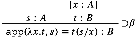
  whose informal reading is as follows: if s is a proof of A and t is a proof of B depending on a proof of A (i.e. a function as unsaturated entity from proofs of A to proofs B) then the proof which one obtains by applying the course-of-values of t to s is the same proof that results by filling the slot of t with s. Although several parts of the material covered in the present work could be naturally reconstructed in the setting of intuitionistic type theory, we prerer to avoid this formalism in order to make the presentation accessible also to readers unfamiliar with it.

• 8. These derivations correspond to the Church encoding of the numerals 0, 1 and 2 in the $\lambda$-calculus. The two derivations of the previous example correspond to the Church encoding of the Booleans.

• 9. Both this example and the previous one rely in an essential way on the availability of the structural rules of weakening and contraction, i.e. on the availability of vacuous discharge and of simultaneous discharge of more copies of one assumption. The implicit availability of the structural rule of exchange also triggers the existence of distinct proofs of certain formulas. For example, formulas of the form $(A\wedge A)\mathbin {\supset }(A\wedge A)$ can be proved either by means of the identity function or by means of the function that maps every ordered pair of proofs of A onto the pair in which the order of the members has been exchanged. The fact that for some formulas there are distinct proofs is however independent of the availability of structural rules. For example, whenever A is some provable formula and $\mathscr {D}$ is a closed $\beta \eta$-normal proof of A, the following derivations denote distinct proofs of $(A\mathbin {\supset }(A\mathbin {\supset }B))\mathbin {\supset }(A\mathbin {\supset }B)$, no matter which formula is taken for B:

  

  Note that in these two derivations no implicit appeal to any structural rule is made. Rather than to structural rules, the availability of more than one proof of a proposition A in $\texttt{NI}^{\wedge \mathbin {\supset }\top }$is closely connected to the number of occurrences of atoms of various polarity in A. As first proved by Mints [106], if a formula A in $\texttt{NI}^{\wedge \mathbin {\supset }\top }$is balanced (which means that each atom in A occurs exatly twice, once in positive and once in negative position) then A has a unique proof [see, for details,122, Sects. 8.4 and 8.5.2–3]. For further references and for a recent investigation on the number of proofs of formulas in presence of disjunction, see Scherer and Rémy [106]. Thanks a lot to Paolo Pistone for a thorough discussion of this point and for providing the example given in this footnote.

• 10. This result is what in the typed $\lambda$-calculus corresponds to a corollary of Böhm’s theorem for the untyped $\lambda$-calculus.

• 11. It is worth stressing that the definition of the notion of isomorphism relies in an essential way on a generalization to open derivations of the ideas presented in the previous section. That is, it is not only assumed that distinct closed derivations in the same equivalence class denote the same proof, but also that distinct open derivations in the same equivalence class denote the same function from proofs to proofs. As detailed below in Sect. 2.7, this generalization is not uncontroversial.

• 12. In calculi in which the replacement theorem does not hold and/or in which transitivity fails, one can define an equivalence relation $A \approx B$ stricter than interderivability by requiring the interderivability of every pair of formulas C and D, such that D is obtained from C by replacing some (possibly all) occurrences of A with occurrences of B (Smiley [106] proposed this notion as the correct analysis of the intuitive notion of synonymy). Observe however that, like interderivability, this notion is also extensional in character, in that it is formulated without making reference to identity of proofs. In calculi in which a non-trivial notion of identity of proofs is available, it is therefore plausible that isomorphism is stricter than Smileyan synonymy.  An example is the natural deduction system for Nelson’s [106] logic $\texttt{N4}$ (see [106], Appendix B, Sect. 2). This calculus is an extension of $\texttt{NI}$ with introduction and elimination rules for the ‘strong’ negation of each kind of logically complex formulas. In $\texttt{N4}$, the interderivability of A and B alone does not warrant that $A\approx B$: A and B are Smileyan synonymous only if both A and B and ${\sim }A$ and ${\sim }B$ are interderivable (where $\sim$ is the strong negation). The relation of $\beta \eta$-equivalence for derivations of this calculus can defined by extending in the obvious way the definition for $\texttt{NI}$ (the generalized $\eta$-expansions to be introduced in Chap. 3 below have to be used both in the case of the “positive rules” of disjunction and of the “negative rules” for conjunction). In N4, A and $A\wedge A$ are Smileyan synoynmous, but they are not $\beta \eta$-isomorphic, i.e. $A\approx A\wedge A$ but $A{\mathop {/\!\!\!\!\!\simeq }\limits ^{\beta \eta }} A\wedge A$. (Note however that in $\texttt{N4}$ an equivalence relation on formulas A and B even stricter than isomorphism could be defined by requiring both $A{\mathop {\simeq }\limits ^{\beta \eta }} B$ and ${\sim }A{\mathop {\simeq }\limits ^{\beta \eta }} {\sim }B$.) Another example of a calculus in which replacement fails is Tennant’s [106] Core Logic. In contrast to what happens in $\texttt{N4}$, in Core Logic no sufficient condition is known that warrants Smileyan synonymy. We conjecture however, that A and $A\wedge A$ are Smileyan synonymous in Core Logic as well. To show that $A\wedge A$ and A are not isomorphic in Core Logic would require the definition of an equivalence relation on derivations in Core Logic. (For some difficulties that might be encountered, see the remarks at the end of Sect. 3.5 and in particular Note 16 to Chap. 3.) If the resulting notion of identity proofs is close enough to the one resulting from $\beta \eta$-equivalence in $\texttt{NI}$, A and $A\wedge A$ would fail to qualify as isomorphic in Core Logic as well.

• 13. This is fully analogous to the role played by $\eta$-conversion in the untyped $\lambda$-calculus—see Note 16 to Chap. 1.

• 14. This weaker notion of $\beta$-reduction is essentially the one advocated by Martin-Löf [106], although with a partly different motivation. As stressed in Note 23 to Chap. 1 and in Note 6 to the present chapter, Dummett [106] gives a different definition of canonical derivations. For closed derivations in $\texttt{NI}^{\wedge \mathbin {\supset }}$, being canonical in Dummett’s sense essentially coincides with being normal with respect to the presenly discussed weakening of $\beta$-reduction. In the present context, Dummett’s claim that canonical derivations (in his sense) are the most direct way of establishing their conclusions can thus be taken to be the claim that closed derivations which are normal with respect to this weakening of $\beta$-reduction are the most direct ways of representing the proofs they denote. As discussed in this section, this is tantamount to adopt an intensional conception of functions and to deny that all instances of $\beta$-reduction are identity preserving.

• 15. What we call $\beta _w$-normal derivations are what correspond to fully evaluated terms in type theory (see, e.g. [106]).

• 16. The fact that the $\eta$-equations express a principle of extensionality for functions is not in conflict with the claim of Sect. 2.6 that the account of harmony based on reduction and expansions is intensional. Reductions and expansions yield an intensional account of consequence (by allowing the possibility of establishing the same proposition by means of different proofs) and of meaning even though the criteria of identity for functions that one adopts are extensional.

• 17. This is at least implicitly done by Dummett, as discussed at the end of Sect. 2.3 above.

• 18. A more general notion of atomic systems allowing rules of higher-level is discussed in [106].

• 19. To check the validity of an open derivation with respect to $\mathcal {S}$ and $\mathcal {J}$ one has to check the validity of all its closed instances relative to all possible extensions of $\mathcal {S}$ and $\mathcal {J}$. As pointed out by one of the referees, it is therefore dubious that the notion of validity can be checked effectively. In some specific cases, it is however easy to show the validity of certain open derivations. A few examples are given in the next section.

• 20. We speak of a generalization since weak reduction was defined for $\beta$-reduction only, whereas here we consider an arbitrary set of reduction procedures.

• 21. The resulting notion of validity could be strengthened, by requiring that all open subderivations of every weak normal derivation obtained from a given one should be valid. Since Prawitz considers arbitrary sets of reduction procedures, there is no warrant that confluence holds, and hence a given derivation may have several different weak normal forms (see [106], for details).

• 22. It is worth stressing that, although Dummett refers to the introduction rules as ‘self-justifying’, strictly speaking they are not correct by fiat, i.e. their validity is not simply stipulated. Both Dummett and Prawitz agree in reducing their correctness to the notion of validity of arguments. However, it is true that given the role played by closed canonical derivations in the definition of validity, introduction rules always turn out to be correct “automatically”.