High-Resolution Delineation of Petroleum NAPLs

Abstract

Previous chapters of this book demonstrate that a cohesive and well-supported conceptual site model (CSM) of non-aqueous phase liquid (NAPL) petroleum is commonly the cornerstone of successful risk analysis and/or remediation design. It is difficult to overstate however, the extent to which the heterogeneity of source term NAPL distribution confounds one’s efforts to develop an accurate NAPL CSM. In most cases, only near-continuous measurements of NAPL in the soil are capable of adequately conceptualizing a site’s complex NAPL distribution. Continuous NAPL logging, conducted at a significant number of locations across a petroleum release site, is necessary to better comprehend the chaotic nature of the NAPL’s distribution. Applying high-resolution screening techniques sitewide is known as high-resolution site characterization (HRSC) and this chapter describes how the most commonly applied HRSC techniques can make the difficult task of logging continuously for petroleum NAPL, and its associated groundwater impacts, not only possible but fairly routine.

8.1 History of Subsurface Petroleum Hydrocarbon Investigation

Regulations regarding petroleum releases in the subsurface were put in place because petroleum contains numerous toxic water soluble compounds including benzene, toluene, ethyl-benzene, and xylenes (BTEX) as well as polycyclic aromatic hydrocarbons (PAHs). These somewhat water soluble compounds partition out of the petroleum non-aqueous phase liquid (NAPL) into groundwater, making groundwater the “canary in the coal mine” at sites where petroleum releases are suspected. If the groundwater is found to be impacted, a petroleum NAPL release has been confirmed.

The first course of action to be taken to determine if a release has occurred has typically been to grab a limited number of soil samples and install the ubiquitous set of monitoring wells, all intended to be placed strategically so as to intercept any dissolved phase contaminants that might indicate a petroleum NAPL release affecting the groundwater. There is little hand-wringing at this stage with regard to what methodologies are employed to obtain samples, because we are initially looking only to find any contaminants of concern (COCs), such as BTEX. We simply sample the groundwater, send it in, wait for the laboratory results, and any decision points are relatively straightforward. Only after finding COCs above a certain threshold in groundwater, confirming NAPL has been released, do we progress to “action levels”. In other cases, NAPL’s presence does not need to be inferred from groundwater contamination, because it is encountered in the monitoring wells, confirming the NAPL’s presence directly.

Historically, the next step of the investigation was to conduct more discrete sampling and more monitoring wells to see “how big the plume is”, kicking off quarterly sampling of those wells, and in general a repeat of previous steps in an ever-expanding fashion. This was often accompanied by a lot of head-scratching as to why some monitoring wells had NAPL, many did not, some contained high dissolved phase, some very nearby did not, NAPL came and went in wells, and so on. Even repeat sampling, at the very same locations but on different dates, produced concentrations that changed wildly. The petroleum appeared to be moving about dramatically with the passing of time.

What was not widely understood at the time was that the majority of sites have very complex NAPL and groundwater flow path architecture. What appeared to investigators as dramatic changes of NAPL and dissolved phase over time were, in reality, mirages caused by natural heterogeneity and/or seasonal or well-induced groundwater movement. For many NAPL release sites, the longer the investigation lasted, and the more wells and soil sampling that was conducted, the more bizarre and contradictory the conceptual site model (CSM) became.

Due to the fact that regulations were focused on the effects to groundwater, the focus for characterization was also on groundwater. These characterizations were often well-conducted, using an array of sophisticated discrete level monitoring wells and sampling systems. This amounted to little more than an advanced understanding of the symptoms of the petroleum’s presence however, rather than the distribution of the root cause itself. This became evident when remedial designs based largely on groundwater data were initially thought to be a successful treatment due to promising declines in groundwater concentrations, but subsequently suffered rebounds in the dissolved phase. Our early focus on groundwater left us with relatively little knowledge about the source term NAPL, for which the applied remedy had little if any efficacy. Add onto that our underappreciation of geology’s tremendous role (especially its inherent heterogeneity) in the early goings of the industry, and it is no wonder that many early attempts at site remediation were destined to be modestly effective at best, and often completely ineffective. It took a long time for the industry to realize that once we had established that NAPL was present in sufficient quantities that it was sourcing a dissolved phase problem, our continued use of methods that focused primarily on the dissolved phases of petroleum no longer made sense. Relying on means designed to measure water, such as monitoring wells that were never designed to measure NAPL, was not sensible.

A familiar adage states that “where there is smoke, there is fire”, and NAPL and its dissolved phase have a similar relationship. Dissolved and vapor phase distribution is helped along by diffusion and groundwater flux, so they behave more like smoke which diffuses freely and is carried by these “winds”. The petroleum NAPL is akin to the fire, moving discretely through soil pores, its path determined by the soil’s grain size, pore sizes, structure, and geometry. And all the while the NAPL is effusing its telltale “smoke” (the dissolved and vapor phase) into adjacent soils and groundwater. NAPL follows a distribution pattern dictated by gravity in the vadose zone, its specific gravity in the saturated zone, and preferential pathways available to NAPL’s viscosity and surface and interfacial tensions, distributed by the whims of geology.

Firefighters faced with finding a fire in a building filled with blinding smoke employ infrared cameras, which allow them to focus on the fire itself and see past the smoke. For similar reasons, investigators seriously interested in understanding petroleum product distribution in the subsurface need to adopt techniques that are highly NAPL-specific in their response, or that are responsive to all phases but continue to increase or otherwise recognizably change their response upon encountering NAPL. As the industry slowly turned its focus to the source term NAPL (not just inferring NAPLs presence by gauging NAPL in monitoring wells and monitoring groundwater) a few early adopter regulators were keen to put their focus back onto the NAPL, in particular relying on direct sensing technologies such as laser-induced fluorescence (LIF) to change their agency’s entire mindsight with regard to petroleum release investigations (Stock 2011).

The term “NAPL body” in context of this chapter means the distribution of light non-aqueous phase liquids (LNAPL) and dense non-aqueous phase liquids (DNAPLs) in the subsurface. This includes both multi-component DNAPLs such as bunker fuel and creosotes as well as the single component chlorinated solvent DNAPLs that often comes to mind when the term DNAPL is mentioned. The term NAPL body as used here includes light staining, those nearly invisible deposits of NAPL that are not readily discernible as free product, discrete ganglia, pools, or droplets. For instance, when one soaks up a diesel spill in the mechanic’s shop with a granular clay-based floor adsorbent, those particles no longer drip or even have a sheen, but they certainly contain diesel’s relatively non-volatile NAPL within their pores, and this NAPL can still act as a source for dissolved phase when the sorbent granules are placed in contact with water. A microscope or other visual magnifier and an ultraviolet (UV) light might be needed to confirm that NAPL exists in fine-textured soils, but indeed it does, and more often than we assume based on examination of cores with the naked eye outdoors in daylight.

The term NAPL body used here expressly excludes the considerably larger plume of vapor and aqueous phase forms created as some fraction of compounds contained within the NAPL emanate away from the NAPL body. It excludes as well those compounds that sorb onto soil particles that they encounter during their convective and/or diffusive travels. This is not to say that sorbed phase contaminants of this nature are not critical sources to consider, especially in the case of more water soluble halogenated DNAPLs such as trichloroethylene (TCE) and the like. These DNAPLs often source enough dissolved phase contaminant, over long enough periods of time, that the remnant sorbed phase adsorbed in low-permeability soils can go on to act as strong source terms via back diffusion, long after the true DNAPL has been depleted (Brooks et al. 2020). This topic has been thoroughly explored, halogenated solvent fate and transport behavior in particular, but back diffusion occurs for petroleum NAPLs as well, just not at such extremes most likely due to attenuation mechanisms deserving of further research. The exclusion of the dissolved/sorbed body from the data set allows one to focus their attention on the originally released source term NAPL, that often is the driver for any continuing sourcing assuming it has not yet been depleted of its water soluble compounds.

The early portion of this chapter focuses on techniques that are capable of generating data that accurately represent this NAPL body either exclusively (NAPL only) and/or the combination of the NAPL body and the associated high dissolved or sorbed phase that is located in relatively close proximity to the NAPL body proper. Of these, only approaches that employ fluorescence spectroscopy can generate semi-quantitative and qualitative responses that are highly preferential to the NAPL body alone. Fluorescence spectroscopy is best able to capture the nuances of the distribution of NAPL body while simultaneously resisting influence from dissolved, sorbed, or vapor phases (there are major departures from this behavior which will be covered). For these reasons, we will explore fluorescence means in the far greater detail and explain how it generates data that accurately represents how the NAPL body has distributed itself and, in some cases, how it can indicate NAPL’s chemistry has changed since its release.

Of these various fluorescence means, time-resolved LIF has the superior semi-quantitative, qualitative, false positive rejection, and monotonic behavior across a wide concentration range and wide variety of NAPL types. Therefore, we will focus on LIF but point the reader to other fluorescence-based means as appropriate.

8.2 High-Resolution Petroleum Hydrocarbon NAPL Screening

8.2.1 Capabilities Necessary to Delineate NAPL

Generating a CSM representative of petroleum NAPL requires tools responding to chemical constituents that are representative of only the NAPL or, at a minimum, tools that indicate NAPL’s presence is nearby (meters), for instance high dissolved phase BTEX. The techniques should also be relatively immune to significant “false positive” responses generated by the soil particles because these materials an be misinterpreted as NAPL (by fluorescence systems). If the system used is not sufficiently immune to responding to false positives, then the system’s response should at least allow for a false positive's recognition as such, in order to allow for their subsequent removal from the NAPL CSM.

Some primary capabilities desired to delineate petroleum NAPLs include:

• Near-continuous collection of measurements.

• Sufficient sensitivity to contaminants/phase of interest.

• Response that is resistant to poisoning/blinding upon encountering NAPL.

• Rejection of false positives (or recognition of them in hopes one can filter their positive response out of the NAPL CSM).

• Ability to access the required depths.

Secondary capabilities that can prove helpful include:

• Monotonic response with NAPL saturation.

• Speciation (insight into changes in the chemistry and/or class of NAPL).

• Speed—the more productive the tool the less it costs, not only in terms of characterization itself, but improved efficacy of remediation as a result of higher data density or more expansive characterization.

• Real-time visualization of results, so adaptive field campaigns can be conducted.

• Minimum production of investigation-derived waste and associated costs.

8.2.2 Choosing the Appropriate Method

Once it has been established that a site would benefit from high-resolution NAPL screening and there is an understanding of what parameters should be measured, a method or ideally set of methods that respond properly to the contaminant (and phase of that contaminant) that is driving your investigation can be selected (ITRC 2019).

8.3 High-Density Coring and Sampling (HDCS)

Traditional core sampling is capable of producing data that can certainly be classified as “high-resolution” and can generate a fully accurate NAPL CSM. However, the equipment, the personnel, and the procedures used for traditional soil sampling did not generally evolve with a focus on NAPL screening. Practitioners who are accustomed to traditional sampling approaches, such as sampling every meter or two or sampling only in targeted intervals (e.g., at the potentiometric surface), have to radically change their mindset if their goal is NAPL delineation. Should they hope to achieve the data density needed to overcome the chaos introduced by NAPL distribution’s heterogeneous distribution that can seem at times to be a mirage, partitioners have to modify their budgets, adjust their expected production rates downward, and generally change the very culture of how they approach sampling. Nevertheless, with careful preparation and mindset it can be done and done well (Byker 2021).

8.3.1 Advantages and Disadvantages of HDCS

Some HDCS advantages are:

• Getting to the necessary depths

Drilling or direct-push systems are almost universally able to get to depth in some manner or another be it auger, direct-push, sonic, or other method.

• Availability

Equipment capable of obtaining subsurface materials is almost universally available around the world.

• Multiple lines of evidence (MLOE)

Even NAPL CSMs generated with direct sensing tools benefit from limited targeted validation sampling. Simply getting one’s hands and eyes on the affected soil can sometimes shed light on why the direct sensing tool has responded the way it has. Geologist’s impressions, screening tool responses, NAPL-indicative dyes, and other methods all contribute to a greater appreciation for core-scale NAPL distribution that is impossible to achieve with one method alone.

An approach perfected over time by numerous skilled researchers and consultants who validated LIF logs to develop confidence in or further the value of LIF-based NAPL CSMs (Ernest Mott-Smith et al. 2014) consists of measuring and recording MLOE, along with photos of cores alongside a measuring ruler. The MLOE data is written with markers onto plastic sheeting or even laminated printouts laid under the core on the processing table (McDonald et al. 2018). This makes note-taking a straightforward and less error prone affair and allows a single photo to capture the entire “data dashboard”. The MLOE data are all generated from narrow fixed intervals so as to spatially align the MLOE with the core, a technique developed to combat severe localized heterogeneity of chlorinated DNAPL during validation studies of dye-based LIF (Einarson et al. 2016). Data dashboard style photography reduces data transcription mistakes (such as typos, mistakes transcribing notebooks to spreadsheets, sample jar labels rendered illegible from shipping damage). Of course, if one is to rely solely on the photography for record-keeping, duplicate photos with two cameras (or perhaps recording the data into a field notebook at the end) are wise. Data dashboard methods can even eliminate the need for further “visualization” of the data in spreadsheets and graphs because it is already spatially organized versus depth in the photo.

Many of the figures depicted in subsequent sections will be using such a data dashboard style to demonstrate the method’s utility for spotting telltale signs of NAPL’s differing behavior from that of other petroleum contaminant phases, and how method can also reveal data misinterpretation mirages for what they are.

• Ability to triage

Screening visually or with handheld photo-ionization detector (PID), dyes, and other rapid screening approaches can be used to identify appropriate intervals for laboratory sample grabs or when to adaptively switch over to high-resolution mode where slower NAPL-discerning techniques would be fruitful. Triaging intervals according to soil core data that is generated with real-time benchtop screening tools allows for adaptive decision-making (deciding on the next sampling locations for instance) because there is no waiting due to shipping samples and laboratory analysis time.

• Familiarity with stakeholders

People trust data generated with “what they know” and are inherently suspicious of techniques they are unfamiliar with. This blind allegiance can at times be irrational and counter-productive, yet it remains that core sampling is often “the easier sell”, especially with stakeholders who are entrenched with doing things the way they have always been done.

Some HDSC disadvantages are:

• Lower productivity

The sampling machinery is often capable of producing cores at a relatively rapid rate, although commonly slower than most direct sensing technologies. Judicious processing of those cores is an additional rate limiting step that greatly reduces production. This is especially true when the core processing is done at a screening density that achieves resolution high enough to assure that small NAPL features (cm to dm scale) are not missed.

• Laboratory costs

Laboratory analysis costs can become prohibitively high even at modest (e.g., 0.3 m) resolution. Great savings can be realized, while still achieving a robust NAPL CSM, by conducting a carefully orchestrated MLOE approach. Selecting occasional grabs for laboratory work at lower density, and using those data to develop an understanding of how these sparser “gold standard” laboratory results relate to the higher density screening methods used, bolsters our confidence in the high-density screening method data. That said, many laboratory methods fail to contribute significantly to the NAPL-only CSM, because they either respond to only select fractions of petroleum hydrocarbons or they respond to all phases contained within the soil, not just the NAPL expressly. It became clear midway through our industry’s development that the regulatory framework had been placing far too much emphasis on “data quality” (laboratory data being the gold standard) to the detriment of data density. This led to the development of the Triad methodology (triadcentral.clu-in.org), an approach to decision-making during characterization that sought to strike a balance between data quality and quantity, giving recognition to the fact that data density was required to overcome the uncertainty caused by spatial heterogeneity of contaminant and hydrogeological properties.

• Skilled labor demands

Judicious processing of cores requires experience and a discipline akin to a military exercise. Assembling such a skilled team costs more than a group of inexperienced personnel. When planning for core screening projects, it is easy to delude ourselves with mental images of the sun shining, birds chirping, good lighting, mild temperatures, and plenty of rest. Reality is often far from this ideal with long hot or frigid days, perhaps some freezing conditions thrown in, making people grow short in patience and encouraging a desire to start taking shortcuts not long into the project. A proper work plan, a sound leader to guide the process, and a crew willing to “stick to the script” is vital. Ignoring the geology (or being lazy toward it) could result in missing a major clue as to how or why the NAPL body has distributed itself.

• Poor recovery and soil disturbance

Years spent validating LIF logs with physical coring has taught us that NAPL has a way of transporting and storing itself in variety of soil types, some of which are very difficult to sample effectively including large gravels, running sands, and the like. It is not uncommon to get full recovery cores all the way down to the interval where the LIF had indicated NAPL, only to have the very core where the NAPL was indicated come back up-hole with only partial or no recovery at all. Direct-push sensing on the other hand typically results in “100% recovery” top to bottom, regardless of the soil’s sampling behavior (outside of refusal). There are methods less prone to recovery issues like sonic drilling but this is often highly disruptive to the contaminant, the soil, or both. Cryogenic coring techniques represent a promising alternative requiring further research and development.

• Investigation-derived waste (IDW)

Conducting HDSC alone to develop a NAPL CSM generates a large amount of IDW compared to direct sensing with limited validation sampling. Depending on the contaminant and regulations, the management and disposal of the large soil volumes necessary to generate a high-resolution model of the NAPL CSM can be expensive enough to be a factor and certainly not the most sustainable solution practitioners should aim for.

• Data handling

Copious amount of data can be generated from HDSC and recording it all is rather daunting and fraught with chance for errors. In addition, site data often gets strung out over many months or years, with change-over in consulting firms or even agencies in charge. In many cases, just a few sloppy errors (or ambiguous observations such as a lone nebulous term such as “impacted” written on a drilling log) can throw doubt onto a data set that had the opportunity to be very insightful but lost value due to poor or inarticulate archiving.

8.3.2 HDSC - Best Practices

• Dedicated workspace

Large table(s) placed in a location where rain, direct sun, and other distracting weather elements are minimized is important. Skilled NAPL delineation practitioners often cover their tables with white disposable plastic and write detailed notes on the table recording the location, depths, geology, NAPL observations, PID response, NAPL sensitive dye tests, and other pertinent data (McDonald et al. 2018).

• Splitting cores

Core liners should be cut lengthwise, followed with splitting of the cores using spatulas, drywall taping knives or similar straight edged tools. Whatever technique is used to split the core longitudinally, it is desirable that the technique retains the interior soil structure. For cores containing loose granular soils, an excellent alternative is to freeze the cores, let the outer liner thaw for a few minutes to reduce brittleness, lay them in a core jig for safety, then cut them completely in half, using stone cutting masonry blades with a circular saw.

Immediately after cutting the frozen cores, one should shave the thin layer of frozen mud off the face of the core to reveal the details of the soil and NAPL distribution. If delineating gasoline or other NAPLs rich in volatile organic compounds (VOCs), it is crucial to keep the core covered in metal foil (never plastic), keep the core cold, and process the cores with as little delay as possible after thawing. Core photography while still in the frozen state works very well, but high humidity environments can cause frost to build up too quickly, obscuring the surface. Freezing cores is obviously not for high throughput, but for cores from important depth intervals, where discovering the details of distribution of NAPL versus the geology is needed.

• Core Photography

Quality photographs record core information in a way that is irreplaceable. If conditions allow it, one should set up a geologist’s UV mineral lamp in a dark room or trailer and take both visible and UV-induced photos. As shown in Fig. 8.1 it is even more effective to mount the camera and core in fixed locations so one can see both the visible and UV from the same perspective. Figure 8.1 contains photos of a 1.2-m long gasoline NAPL-impacted soil core photographed under various conditions. The cyan blue is gasoline NAPL fluorescence, the purple hue is reflected UV lamp visible color bleed, and the creamy orange is fluorescence of an indicator dye (indicating the most freely available NAPL). The bottom of the core is at right and the arched patterns in the fine laminar soil layers were caused by higher sampler friction on the outer soils. The narrow black lenses in the visible photograph at bottom are a seam of granulated activated carbon amendment.

Fig. 8.1

A soil core that has been frozen and cut in half lengthwise. From top to bottom are UV with indicator dye (orange), UV, and visible lighting conditions

Keep in mind that kerosene (jet fuel), aviation gasoline, bunker fuels, and other NAPLs are difficult if not impossible to document properly with UV-excited photographs because they simply do not fluoresce appreciably in the visible wavelengths.

• Subsampling

Composite sampling, by design, generates an “average” response across the soil column. Subsequently, it fails to provide any insight into the nature of the NAPL’s distribution and/or degree of heterogeneity. The narrower the depth interval sampled, the more accurately it represents the extremes that NAPL is typically capable of achieving across short distances. Subsampling with Encore samplers (or syringe bodies with the needle attachment cut off) combined with inexpensive screening tools such as dyes, glove tests, PID, and others, which generate data consistently and rapidly for little cost, is highly desirable to learn about how NAPL distributes itself in the soil. A small fraction of these numerous samples are often co-sampled at the same horizon as other tests and are sent in for formal laboratory testing.

• Indicator dyes

Shake tests consist of adding hydrophobic indicator dyes and water to soil samples in a jar that is shaken briefly and then examined. The dyes change color only when they dissolve into an organic liquid and they are particularly good for testing for NAPL presence. Unlike laboratory or PID readings, dye tests are much more decisive because they are reacting to a physical transformation of the hydrophobic dyes that only become colorful when NAPL has solvated them, regardless of sorbed or dissolved phase concentrations in the soil core. Oil Red O and Sudan IV are famously used in the chlorinated NAPL sector (Cohen et al. 1992), and companies sell various colored dye “kits” that make the test easy to implement properly with relatively little experience. Buying scintillation vials and bulk dyes and doing it yourself is much cheaper and achieves excellent results (Einarson et al. 2018). Most NAPLs respond well, but NAPLs that are very dark or black (such as coal tars and tank bottoms) will almost certainly not respond due to the absorbance of light by carbon and other chromophores that quench or physically filter out any nuanced color changes. One should also be careful of assessing a “light positive” response caused not by dye dissolving into trace NAPL but is instead simply grains that are the same color as the dye when it contacts NAPL. In cases where even trace NAPL is of interest, it is best to have a vial of control soil placed next to the jar to which indicator dye has been added, so flecks of soil coincidentally shaded in the same color as the dye change are more easily appreciated and assessed as soil, not NAPL positives.

• PID

Inexpensive handheld PID devices are useful for screening of VOCs that are either in NAPL form or are emanating from dissolved or sorbed phases typically located close to source NAPL. PIDs are often used in headspace mode, where a sample is placed in a container and the headspace is measured. For NAPL screening, the abundance of VOCs may allow a more direct continuous “sniff” along the cores surface, insertion into a series of shallow divots, or cupped with a clean gloved hand to help assure the VOCs are only emanating from the core section being screened. In this way, rapid progress can be made along the core until the PID alerts the screening team to go from their relatively “coarse” sampling (along with geologic examination) to high-resolution subsampling.

• Glove stain test

Testing for NAPL by looking for staining of nitrile gloves with NAPL is an inexpensive and reliable test for NAPL, because only NAPL can move directly and rapidly into the nitrile polymer and stain it, unlike the vapor and dissolved phase, soil, and/or water. Exposing the glove to NAPL-free soils, then washing the glove with soap and water and rinsing, will result in a stain-free surface. But exposing the glove even to sheen traces of NAPL will result in NAPL collecting into the glove’s polymer (a process called solid phase extraction). A glove also allows one to work the glove into dark, fine, and opaque soils and sediments, where visual detection or dyes are notoriously ineffective, allowing one to search around for any NAPL droplets. When used in this manner the glove is sampling far more soil than surface-based techniques, allowing for more exhaustive detection of any NAPL present. A light-hued glove, in particular light green, is a popular choice. It might seem like an amateurishly simple technique, but for many NAPLs the glove test can uncannily discern NAPL when dyes, photos, or the human eye cannot.

• Shake tests

Placing soil in a container with water and then shaking the mixture causes NAPLs to free themselves from the soil and float on the water’s surface. This is a reliable technique for most NAPLs, but stiff cohesive soils like clays are often difficult to disperse enough to free up much NAPL. Letting the water settle for some time greatly aids detection of NAPLs versus trying to detect them under turbid conditions. One should be aware that exceptionally clear NAPLs remain challenging at lower saturations, and that some NAPLs collect on the glass as opposed to forming a visual sheen or layer at the water’s surface.

• Concise language and terminology

Nothing is more frustrating than having gone through exhausting and expensive high-resolution core screening process, only to find that the processing team’s terminology and decision-making was inconsistent. Vague simple terms like “impacted”, “odor”, and “saturated” should be more specific, such as “NAPL-impacted (sheen)”, “aromatic odor”, and “groundwater saturated”. Degree of impacts should be kept on a simple coarse scale of perhaps zero to three or four. Handheld instrument responses can then be normalized to that same scale—allowing for all the data to be hung vertical on the same axes, using differing colors or symbols for each line of evidence. This normalization makes it easy to see when and where the various lines of evidence agree (building confidence) or maybe even highly disagree, perhaps pointing at a NAPL that is present but has dramatically different chemical properties than the target NAPL originally being delineated. For instance, a chemically intact gasoline NAPL will cause a high response to PID, glove, and dye while a clear mineral oil might cause a poor PID and glove response, but a vivid dye response.

8.3.3 HDCS Logging in Practice

Figure 8.2 represents an idealized scenario of a boring location continuously cored and screened for gasoline NAPL. Figure 8.2 incorporates a number of elements that are routinely encountered during a typical NAPL-specific screening exercise. As previously stated, the relationship between multiple lines of evidence can be exceedingly difficult to conceptualize unless they are all hung together and graphed vertically. MLOE “data dashboard” figures like Fig. 8.2 help us make sense of different data types which sometimes contradict or support each other. Various depth intervals (listed alphabetically at far right) have been selected for discussion so as to help the reader identify commonly encountered situations that often lead to misinterpretation or underappreciation of the meaning of data produced with high-resolution techniques.

Fig. 8.2

Idealized scenario of NAPL and VOC distribution in the soil column with MLOE data resulting from HDCS methodology

Key elements to consider in Fig. 8.2 include:

• The four columns at far left (Soil Profile, Gasoline NAPL, and VOCs) represent the true soil profile in this scenario. If the HDCS techniques used to generate MLOE data perform ideally, the MLOE data at right (PID, Dye, Lab, and UV Photo) should match what is pictured in the idealized “reality” in the four columns on the left.

• The idealized columns at far left will be held static throughout the discussion of HDCS, MIP, and LIF methods in subsequent sections, so that one can appreciate the differences between the methods when they are applied to identical soil and NAPL conditions.

• The VOCs column describes total VOCs (e.g., BTEX) versus depth and is plotted in log format. This is necessary because while VOCs dissolved in groundwater, soil pore gases, and sorbed phase near NAPL can reach significant levels, the concentration of these non-NAPL phases of VOCs is dwarfed by their relative abundance in NAPL proper. Notice in Fig. 8.2 how VOCs are encountered throughout the entire soil column shown, because VOC components are always more widely and homogeneously distributed than NAPL.

• The NAPL column contains various forms of NAPL—ranging from fairly saturated and obvious in a soil core to very light staining that might be difficult for a geologist to identify visually.

• The density of the sampling intervals shown here was arbitrarily chosen. We are not suggesting one typically sample 50 intervals at each location, but then again it does occur. Sampling density is a balance of budget, time, and goals.

• Notice the switch from coarse sampling intervals to narrow intervals (and NAPL-specific methods) took place only after the PID threshold was exceeded. Time and money were saved by screening at coarser intervals only with the PID.

• Intervals A and C were screened at high-resolution and included the more laborious NAPL-specific methods, the dye shake tests (Oil Red O in clear vials), and UV photos. Once the PID threshold dropped back below the action level, the coarser spacing was resumed. A glove staining test would probably not have provided an acceptable alternative to the dye test for fresh clear gasolines but would for many discolored or heavier NAPLs.

• Interval A contains perched NAPL sitting on clay according to the MLOE, but UV photography only indicated NAPL in the top half of the NAPL lens due to the clay’s fine grains’ ability to hide NAPL fluorescence relative to sand (Apitz et al. 1992) and/or the difficulty of NAPL to penetrate fine-textured soils.

• Both the dye testing and the UV photos indicated NAPL at intervals A and C. These positive NAPL responses were corroborated by substantially elevated concentrations in the validation laboratory samples grabbed at intervals that were indicated to contain NAPL.

• All four MLOE data streams in interval B agree that while VOCs were modestly present, no actual source term NAPL exists. The laboratory samples confirm that the screening tools are responding appropriately (i.e., not exhibiting falsely negatives for NAPL). This illustrates the utility of confirming both low and high responses, not just the highs.

• Looking closely at interval C’s MLOE data versus NAPL saturation, it is clear that NAPL was encountered, but the depth at which it registered in the MLOE data is deeper than our model’s “reality”. Simple human error, compression of tooling, drilling issues, and a host of other factors often lead to improperly determining the depth of the core material and thus the depth to NAPL. These depth mismatches are a common thorn in the side of everyone who validates direct sensing with HDCS.

• Interval C contains the classic “shark’s fin” NAPL saturation that appears in homogeneous sandy soils with a stable phreatic surface (Tomlinson et al. 2014). Partial NAPL saturations often result in “pink” red dye tests rather than bright red. A laboratory sample grab at the same interval as the slightly positive pink dye shake test is implemented confirms the modest level of NAPL impact indicated by the light pink (less than obvious) dye response.

• Interval D contains a significant lens of NAPL trapped below clay in running sand, but this was not discovered by HDCS due to lack of recovery of the running sands. This is a common occurrence because NAPLs often reside in difficult-to-sample soils.

• Interval E was submitted for laboratory analysis in order to generate data on the low end of the petroleum contamination spectrum, without which the behavior of the MLOE screening tools cannot be fully validated with respect to false negatives. False negatives are notoriously easy to ignore because investigators may think that certain depth intervals are NAPL-free, but until and unless it has been demonstrated it is premature to assume so.

• Notice that the fluorescence photo colors change with depth, not only between the false positive calcite and NAPL, but within various horizons of the gasoline NAPL itself. These color changes are the result of significant chemistry changes. It is common for perched gasoline near the soil surface to weather significantly, and that is illustrated in this model. Notice in the UV Photo column that the NAPL deposit at interval A is turquoise (weathered) in contrast to the bluer (inferring a more intact) gasoline NAPL at interval C. The top side of interval C also weathered to a turquoise color similar to interval A. How NAPL fluorescence colors vary and can change, and the significant role that colors can play in identifying NAPLs, discerning false positives, and identifying weathering will be detailed in the LIF discussion sect. 8.6.3.1.

8.4 Direct Sensing of Petroleum NAPL

Early pioneers of geotechnical soil assessments developed simple probes that were pushed steadily down into the soil, without rotation, while measuring the probe tip’s resistance. This cone penetration test (CPT) method was later enhanced with the addition of a friction sleeve and eventually pore water pressure sensors. CPT systems have gone on to revolutionize geotechnical characterization and the speed at which geotechnical data can be gathered. Researchers at the United States Army Corp of Engineers Waterways Experimental Station (WES) added a sapphire window to the side of their probe in the early 1990s to enable detection of petroleum hydrocarbon NAPLs by their fluorescence. Percussion delivered direct-push sampling platforms were developed and gained popularity in the late 80s and early 90s. Researchers and probing companies subsequently developed and manufactured sensor systems that allowed percussion delivered direct sensing of contaminants in situ. Like the geotechnical revolution prior, the ability to measure petroleum chemistry continuously with depth greatly advanced the field of subsurface petroleum hydrocarbon characterization.

There is a myriad of tools and sensors available for characterizing aqueous phase (groundwater) hydrocarbons, but this chapter focuses on two mainstream direct sensing technologies that are capable of characterizing the source term NAPL and/or the high dissolved phase that indicates source term NAPL is close by. The next sections will discuss the Membrane Interface Probe (MIP) that measures the VOC fraction of NAPLs exclusively, which is pertinent to gasolines whose formulation is complex and forever changing with regulations and technology (Chin and Batterman 2012), and will more closely examine LIF which is essentially blind to the VOCs and responds instead to the PAHs (semi-VOCs and non-VOCs) that are mostly contained within the source term NAPL itself. These two major classes of petroleum logging tools both directly sense petroleum contamination but come at the problem from very different chemical perspectives.

Fig. 8.3

MIP transports VOCs to uphole detectors via tubing with the aid of carrier gas flow (after figure courtesy of Geoprobe Systems)

8.5 Membrane Interface Probe (MIP)

The MIP is a VOC-sensitive direct-push delivered tool manufactured by Geoprobe Systems^® (Salina, KS, USA). It screens for VOCs continuously and rapidly, much like a handheld VOC sensor, but with the major advantage of being combined with a durable steel tool that can be hammered into the ground where VOCs are measured in situ (Christy 1996; ITRC 2019). As illustrated in Fig. 8.3, carrier gas is introduced into small tubing (preferably polyether ether-ketone or PEEK) that delivers the gas down to a heated gas transfer port built into the side of the direct-push delivered probe. A durable metal-supported hydrophobic polymer matrix shields the carrier gas from intrusion by water, NAPL, and solid particles while allowing VOCs and semi-VOCs to pass though into the carrier gas stream, where they are subsequently carried back uphole and into a series of detectors usually housed in a gas chromatograph instrument. A heater block consisting of a resistive heater coil and a thermocouple holds the membrane’s support fixture at the set temperature (normally 120 °C) which warms the membrane and surrounding formation. The high temperature hastens the diffusion of analytes across the membrane and into the port and also serves to drive off VOCs or semi-VOCs that may cause a residual response when the probe is advanced downward into less impacted soils.

The VOC transfer rate across the membrane generally trends with VOC content of the formation, but factors such as grain size may influence the pressures outside the probe and the transfer rate of VOCs across the membrane (Costanza et al. 2002). As such, low-permeability materials such as clays are thought to enhance the VOC transfer across the membrane, while high-permeability materials decrease it (Costanza et al. 2002). The probe is typically advanced at 30-cm (1-ft) intervals. At the end of each interval, advancement is paused (generally for 45 s) while the MIP’s heater block and membrane reach the desired temperature and heat the surrounding formation, after which the probe is again advanced to the next depth. VOCs are capable of crossing into the probe at all times, but maximum transfer typically occurs as the temperature of the membrane and adjoining formation approaches the heater block target temperature.

As mentioned, the sensing of the VOCs that cross into the probe does not actually take place inside the probe—although successful implementation of downhole halogen-specific detector (XSD) has accomplished down-hole detection of contaminants in membrane interface gas flow (Lieberman 2007). Typically the VOCs are transported uphole by an inert carrier gas (normally nitrogen) via tubing that is incorporated into a trunkline of carrier tubing and wires that have been pre-strung through the direct-push rods. Transport to the surface allows for the vapors to be introduced into a climate-controlled housing, where the analyte gas stream is dried of interfering water vapor (generally using Nafion™ tubing and sometimes a water trap) and passed through multiple detectors. The climate-controlled housing assures that the sensors and electronics are stable and able to respond properly under field conditions where ambient temperatures range widely.

A trio of sensors is typical and includes a PID, a flame ionization detector (FID), and an XSD, although alternative configurations have been used with the objective of improving the qualitative and quantitative interpretation of MIP results [e.g., (Bumberger et al. 2016)]. Proper interpretation of the various detector responses enables stakeholders to identify the main classes of VOCs the MIP is encountering at various depths, and gain insight into the relative concentration of VOCs in the formation. Data generated by multiple detectors can also function to identify false positives such as methane which is produced during biodegradation of hydrocarbons and natural organics such as buried wood and vegetation.

Before and after each MIP log, the MIP practitioner will run chemical response tests using compounds of concern at a known concentration to evaluate response consistency of the primary detectors and to calculate the gas trip time by measuring the time required for the detectors to respond after the membrane was exposed to the chemical standard.

Transporting the VOCs back to the surface for detection by sensitive and reliable detectors is advantageous but employing a permeable membrane and tubing for this purpose also creates challenges. Petroleum hydrocarbon NAPLs are an extremely complex assembly of molecules, with each individual compound having a unique volatility, as well as some degree of affinity for the membrane and/or the transport tubing’s interior surface, depending on the molecule’s size and structure. Consequently, many gases spend considerable time adsorbing to and then desorbing from, the membrane and interior surfaces of carrier tubing during upward transport. Generally speaking, the higher the molecular weight and boiling point of the molecule, the longer the tubing travel (retention) time, resulting in a behavior similar to that observed in chromatographic columns. The most volatile compounds experience a rapid and relatively unencumbered transport to the surface, while sequentially heavier VOCs and semi-VOCs arrive later and may remain stuck in the colder carrier tubing for hours. Some may never clear (cold trapping), in particular where the MIP was delivered through heavier (diesel or crude oil) NAPLs. This may even result in carrier lines needing to be discarded and replaced.

Water vapor also passes through the heated membrane and travels to the colder carrier tubing, where it can condense to form a film of water that can act as an additional stationary phase, exaggerating the chromatographic behavior. Low-permeability formations may enhance this problem by generating higher membrane exterior gas pressures (Adamson et al. 2014). Decreasing the heater block temperature down to 95–100 °C has been proposed to reduce water ingress into the probe and trunkline, although this adjustment may simultaneously contribute to the risk of blocking the carrier tubing by lowering the gas temperature. A heated trunkline version of MIP was introduced in 2009 to alleviate some of these issues, as well as to increase the contaminant transport rate through the trunkline, by maintaining an elevated temperature in the tubing. Heated carrier lines are made of stainless steel instead of PEEK, which makes them harder to manipulate in the field. One situation where the heated trunkline MIP appears to offer a great advantage is operating in sub-freezing weather, because it prevents icing of water vapor condensate in the carrier tubing that can block gas flow.

A common consequence of trunkline carryover is that MIP detector responses often remain elevated for some time after the probe has passed through significant contamination (NAPL) and advances into intervals with lower contaminant concentrations. This is because heavy loads of NAPL-sourced analyte gases are still adsorbed to the walls of the tubing and will continue to bleed out over time. If the probe is still being advanced during this carryover response, it appears to the observer that “dragdown” of the contaminant is occurring. The heavier the molecular weight of the contaminant encountered, and/or the greater the contaminant concentration encountered, the more severe the trunkline carryover issue. Gasolines vary in their formulation chemistry as well, with some gasoline chemistries exhibiting little carryover, while others can cause noticeable carryover if significant concentrations were encountered by the probe.

There are operational tricks that experienced MIP operators have to reduce the complications caused by carryover. If the carryover is significant, MIP operators often pause the advancement of the probe to allow the carrier line to clear so as to better define the contaminant distribution below highly contaminated intervals. During this pause, the temperature of the probe and the carrier gas flow may be increased to flush the residual contamination from the system (Adamson et al. 2014). If the petroleum loading of the carrier tubing is severe, the wait can take hours. MIP providers have also learned to approach the suspected location of LNAPL bodies (gasoline for example) from outside the suspected LNAPL limits, moving carefully in toward the potential source LNAPL. They can safely approach from the outside because the predominantly smaller and lighter molecules that are water soluble (the symptom of the LNAPL source) naturally also have a lower affinity for the carrier tubing’s interior wall. Another option MIP operators have is to increase the setpoint temperature on the MIP probe from 120 to 140 °C, which will reduce the number of heat cycle events required to desorb analytes off of the MIP membrane and move them into the carry gas stream. This may improve the delineation of the contaminant profile especially when encountering LNAPL, although it may simultaneously increase the risk of water ingress and condensation. MIP trunklines might also include two carrier return lines, allowing the operator to switch to an uncontaminated one while the other clears.

Increasing the push rate and/or the carrier gas flow in highly contaminated intervals are other ways of reducing the diffusion rate of LNAPL constituents through the membrane and try to prevent saturation of the gas lines and chemical detectors. Using relatively short trunklines may also contribute to decrease the risk of cold trapping. MIP practitioners generally try in earnest to avoid getting into significant saturations of LNAPLs and generally attempt to avoid any encounters with medium weight LNAPLs like diesel. Encounters with even heavy NAPLs such as crudes will typically result in long-term or even permanent trunkline contamination, so use of MIP at sites suspected of involving NAPLs heavier than gasoline is often not advised.

The ensuing carryover prevents the rapid drop in response that should be observed as the probe moves out of the LNAPL down into non-LNAPL containing soils. Thus, the MIP often delineates the top of the LNAPL body adequately but is quickly blinded by the high response, rendering it unable to determine the bottom of the LNAPL impacts. This has led researchers to investigate the carryover phenomenon carefully and even investigate if perhaps the top and bottom of highly contaminated intervals might best be delineated using multidirectional MIP screening (Bumberger et al. 2012) and even methods that utilize a secondary carrier tube (Bumberger et al. 2016) that can be switched over to prevent carryover effects and which could also enable improved logging of low contaminant concentrations as achieved with low-level MIP systems.

8.5.1 MIP Logging in Practice

Figure 8.4 features the same idealized scenario used in Fig. 8.2 but with MIP direct sensing applied rather than HDCS to compare the MIP’s response versus the true contaminant distribution defined by our idealized in situ condition model.

Fig. 8.4

Idealized scenario of vertical NAPL and VOC distribution with hypothetical PID and FID detector data from MIP direct sensing

Key elements of Fig. 8.4 include:

• The VOCs column represents BTEX and short-chain aliphatics, in other words, the volatile fraction of gasoline that MIP detects well. The idealized VOC profile includes VOCs in all phases, including the NAPL, dissolved (aqueous), volatilized (gas), and sorbed phases.

• While the MIP has a variety of detectors, this scenario shows only the PID and FID. In cases involving only petroleum (e.g., gasoline) without halogenated additives, the XSD would not give response, so it has been omitted here.

• The FID is superior to the PID when attempting to define the NAPL because it is less sensitive at lower concentrations but has a wider dynamic range and top end response. An FID response exceeding 1 × 10⁷ µV is considered by many to be indicative of NAPL. The PID is less NAPL-predictive because it typically experiences greater carryover effects than the FID, thus limiting its ability to delineate NAPL-impacted intervals. The PID is also more sensitive and it may enter detector saturation territory well before true NAPL is encountered, although the detector and computer gain settings can be adjusted before the detectors reach a level that exceeds their maximum output signal.

• The (admittedly cartoonish) “spikes” rising out of the MIP response at semi-regular intervals are due to momentary increases of VOC flow crossing the membrane during the ~ 45 s pause every 0.3 m. With the probe’s downward motion paused, the membrane and the formation in the probe vicinity warm rapidly, creating optimal VOC transfer temperatures and causing the VOC transfer spike. This is followed by the rapid depletion of the VOCs at the membrane’s immediate exterior.

• Interval A shows the MIP’s positive and growing response to VOCs associated with NAPL’s nearby presence.

• In interval B, the MIP passes into a modestly saturated lens of gasoline NAPL perched on a clay lens, evidenced by the sudden increase in MIP response. The PID saturates quickly while the FID increase better reflects the extent of the NAPL. In addition, the transition into clay resulted in more backpressure and the associated increase in the response versus the medium sands. The FID still has “room to run” so its response increases, while the PID rise is dampened by its maximum output signal using the default detector (high gain) settings.

• In interval C, the VOCs actually drop off quickly, but the PID response is affected by carryover in the tubing. The carryover shown in the FID is less pronounced because of its more NAPL-selective response.

• Interval D represents a scenario that MIP practitioners commonly try to avoid, contacting enough NAPL in the pore space to source a sustained high flow of VOCs. The PID response is saturated and the relatively massive increase in VOCs associated with high NAPL content is shrouded in this saturation state where the response simply cannot go any higher. The FID response better depicts the NAPL-impacted interval.

• The FID’s high response and lengthy and sustained PID carryover in interval E is indication enough that substantial impacts (NAPL) were encountered. In many cases, the MIP logging might be paused at interval E to allow the trunkline to clear. In this case, probe advancement is continued for demonstrative purposes. Notice also that the VOC profile is tailing away slowly under the NAPL in interval D contributing to the high PID responses. The FID, again, shows better fidelity to NAPL.

• In interval F, the clay lens and subsequent transition into NAPL in running sands causes another increase in response. However, the NAPL’s presence (especially for the PID) remains shrouded in the saturation and carryover from interval D, so recognition of this NAPL is uncertain.

• In interval G, higher adsorption capacity clay causes heightened MIP response, due to the increase in VOCs available to desorb into the membrane. As discussed, there is also evidence that MIP response varies with sediment type, not just concentration (Costanza et al. 2002; Adamson et al. 2014; Christy et al. 2015) and that less-permeable materials (e.g., clay) may generate increased partial pressures outside the membrane versus sands, which improve VOC transfer across the membrane. Accordingly, no matter what type of sensors are being evaluated it is difficult to design and conduct laboratory and field experiments that are capable of parsing the numerous parameters that contribute to MIP and other in situ sensor responses occurring deep underground.

In summary, MIP remains the premier tool for in-situ delineation of total petroleum VOC contamination and it is useful for certain volatile petroleum NAPL delineation tasks, but one must keep in mind how some factors, including the presence of NAPL and other highly contaminated intervals, may impact the MIP results. Figure 8.5 illustrates this point well and contains MIP data that was gathered at a petroleum (gasoline) filling station in 2018. Notice that the MIP’s PID and FID responded to VOCs almost continuously with depth, while the XSD stayed low, assuring investigators that halogenated compounds were not encountered. The contribution from all VOC phases, combined with modest trunkline carryover (red lines), caused responses that looked like physical contamination “dragdown” outside the probe. Despite their diminutive size, the tiny NAPL deposits, in Fig. 8.5, sourced enough VOCs in their various forms to the surrounding soils to assure a robust MIP response across the entire span of VOC-affected soils, while they were only modestly above the minimum detection threshold for the LIF system as shown in the LIF log at right. Subsequent coring adjacent to these MIP and LIF locations (< 1 m) confirmed the presence of randomly distributed discrete NAPL weeps from pinhole-sized features in the silty soil. These weeps were photographed after they produced a sheen across the core’s face in the UV-induced photographed at right. Further information on LIF is provided in Sect. 8.6.

Fig. 8.5

Co-located MIP and LIF logs acquired at a gasoline release site

8.6 Laser-Induced Fluorescence (LIF)

LIF is an analytical technique applied across a host of disciplines, including drug discovery and genomics, not just contaminated site characterization. The technique consists of directing laser light at fluorescent molecules which absorb some of the light, which excites them, ultimately inducing them to emit light that indicates the molecule’s presence. Most petroleum-based NAPLs such as fuels, oils, coal tars, and creosotes contain enough naturally fluorescent molecules such as PAHs (Berlman 1965) to allow for the NAPL’s detection using LIF. LIF responds almost exclusively to fluorescent molecules that reside primarily in the NAPL and thus in-situ LIF measurements have not been found to be significantly responsive to gaseous or aqueous phase contaminants in the pore spaces.

As depicted in Fig. 8.6, LIF is typically deployed with direct-push tooling. As the tool is steadily pushed into the unconsolidated formation at 2 cm/s, brief (~1–2 ns) pulses of laser light are carried by a fiber optic down to sapphire window in the side of a steel probe (see Fig. 8.7), where it is directed out the sapphire window in the side of the probe, causing fluorescence to be emitted wherever NAPL-affected soil (or any other fluorescent material) is encountered. Laser light is directed at the formation soil that is pressing hard up against the outer surface of the sapphire window and while there is some slight penetration into the pore spaces, penetration is limited to approximately 1 cm in depth at most in favorable conditions (e.g., transparent coarse sand grains). The intensity of the fluorescence induced in the formation generally scales with NAPL impact, but is affected by other factors described in the following paragraphs. A portion of the fluorescence couples back into the probe through the window and is carried back up to the surface by a second fiber optic cable, where the returning fluorescence is dispersed according to color and detected versus time (temporally) with a photomultiplier tube. In this fashion, direct-push LIF provides rapid and cost-effective delineation of most petroleum NAPLs.

Fig. 8.6

A conceptual illustration of conducting LIF characterization of NAPL at a site where two differing NAPL bodies have co-mingled

Fig. 8.7

Laser-induced fluorescence probe concept. PMT stands for photomultiplier tube

Production rates often exceed more than 10 locations per day (depending on probing conditions), yielding cost-effective high-density fluorescence data that can then be displayed as singular logs, series of logs taken across transects (fence diagrams), or 3D visualizations to give a quick idea of the distribution of the NAPL sitewide. LIF is often coupled with other downhole tools on the same tool string (e.g., electrical conductivity or a continuous direct-push injection logging module; see Chap. 7 for more information on these technologies) allowing the investigator to gain a better understanding of how the site geology is controlling the NAPL distribution. Cobbles, gravels, caliche, and other difficult to penetrate materials often limit the attainable depth and sometimes make direct-push logging impractical.

8.6.1 History

Early development of continuous wave (non-lifetime) LIF technology began at the United States Army Corp of Engineers’ Waterways Experimental Station (WES) in the early 1990s. It is with the Naval Research, Development, Test and Evaluation Division, they initially developed a system that relied on a downhole mercury lamp to excite the PAH compounds in situ and was delivered into the subsurface with cone penetrometer direct-push technology. The mercury lamp was later replaced by light from a 337 nm wavelength laser delivered via a fiber optic to the subsurface. The fluorescence was transmitted back to the surface with another fiber optic to an optical multi-channel analyzer (OMA) which measured the spectral and intensity properties of the returning fluorescence (Lieberman et al. 1991). This system was one component of the Site Characterization and Analysis Penetrometer System (SCAPS) (Knowles and Lieberman 1995) and it was well suited to detecting medium-to heavy-weight fuels like diesel and crude, but performed less satisfactorily on gasoline and was nearly blind to jet fuel (kerosene), which was a major contaminant of concern of the U.S. Air Force (USAF).

The USAF coincidentally had been working for several years with North Dakota State University to develop a system that employed a pulsed tunable dye laser capable of emitting the shorter wavelength energies (260–290 nm wavelength) required to excite and detect the fluorescence of BTEX and naphthalenes in groundwater using fiber optic probes (Meidinger et al. 1993). At the request of the USAF, the system was modified to allow its use to include measuring NAPL on soils through the sapphire window of a CPT system. Research field trials showed promise and the system was commercialized as the Rapid Optical Screening Tool (ROST™) by Dakota Technologies, Inc. (Fargo, ND, USA) in 1994 (Nielsen et al. 1995). A subsequent generation system that utilizes a fixed wavelength xenon-chloride excimer laser (308nm) for excitation was developed by Dakota Technologies, Inc. in 2005 and is currently marketed and sold under the brand name Ultra-Violet Optical Screening Tool (UVOST^®). In 2004, improvements on the core technology were made to optimize LIF’s performance for coal tars, creosotes, and other heavy NAPLs, leading to a new generation of optical screening tool (OST) that was branded the Tar-specific Green Optical Screening Tool (TarGOST^®) (St. Germain et al. 2006; Okin et al. 2006). In 2010, Dakota teamed with consultants to develop and test a concept that had been conceived of by U.S. Navy scientists but never put into practice. A fluorescent NAPL-indicator dye injection system was added to LIF in order to induce non-fluorescent NAPLs (including chlorinated solvent DNAPLs and monoaromatic NAPLs such as benzene and toluene) to fluoresce, and this model was branded as the Dye-enhanced Laser-Induced Fluorescence (DyeLIF™) system and has been offered to the industry since 2014 (St. Germain et al. 2014).

While numerous researchers over the years have proposed optimal laser and detection wavelength systems for in situ detection of various classes of NAPLs in situ in the last 30 years, Dakota Technologies, Inc. remains the only company to have commercialized time-resolved LIF systems through both sales of systems and characterization services. Unfortunately, optimizing a fluorescence system to detect the unique chemistry of any specific NAPL type is often accompanied by a significant sacrifice in that system’s ability to detect other types of NAPL because each NAPL type requires unique excitation and fluorescence emission combinations for optimum performance (Kram et al. 2004; Kram and Keller 2004; Kram and Keller 2004). While a universally responsive system is technically feasible, the prohibitive cost and complexity of such a fully capable machine is currently beyond the industry’s ability to financially support its development. Over the decades, government and industry funded research, in combination with field implementation at thousands of sites, has eventually led to the creation of a “family” of LIF systems that strike a balance between optimized detection of some particularly important classes of NAPL without overly sacrificing their ability to discern other classes of NAPLs and/or false positives.

8.6.2 LIF Family of Optical Screening Tools

There are currently three LIF systems and each strikes a balance between specialization and broad applicability. Figure 8.8 illustrates how the three types of LIF fit in with the wide variety of NAPLs commonly released into the subsurface and in need of delineation for risk assessment and/or remedy design.

Fig. 8.8

Laser-induced fluorescence systems and their optimal NAPL detection performance

• 1. UVOST: This time-resolved LIF system has excitation and emission capabilities optimized for use on light to medium weight petroleum fuels and oils. Specifically, the UVOST employs a 308-nm XeCl laser, which produces 1–2 ns duration pulses of light to excite PAHs (and false positive non-NAPL fluorophores should they exist). UVOST detects ultraviolet to blue color fluorescence versus time, resulting in data called waveforms. Under optimal conditions, UVOST responds monotonically to LNAPLs that are commonly encountered at gasoline dispensing stations, military fuel depots, refineries, pipelines, and bulk handling facilities. Heavy molecular weight NAPLs (“heavies”) such as coal tar or bunker at far right in the figure will likely be vastly under-reported (very weak response) with UVOST, but it is not likely for heavies to generate true false negatives (no signal whatsoever).

• 2. TarGOST: This LIF system uses a pulsed (1–2 ns duration) 532-nm wavelength laser to excite the very large PAHs in heavy NAPLs that all UV-induced fluorescence tools struggle to detect. Heavy NAPLs are often multi-component products with densities equal to or higher than water, and this NAPL group includes coal tars, creosote, tank bottoms, bunker fuel, and similarly dark highly recalcitrant NAPLs.

• 3. DyeLIF: This is a time-resolved fluorescence system optimized for detection of chlorinated solvent DNAPLs and other solvent NAPLs that are not naturally capable of fluorescing due to their lack of PAH content. DyeLIF is spectroscopically similar to TarGOST but is aided by injection of a fluorescent indicator dye that stains colorless NAPLs, causing them to fluoresce. The dye functions as an insurance policy that promotes fluorescence to occur in cases where non-fluorescent NAPLs do not fluoresce enough to allow for confident detection.

All three LIF systems shown in Fig. 8.8 are relatively blind to certain NAPLs (false negatives). UVOST, for example, which is designed to characterize light to medium weight fuels, is nearly unresponsive to many coal tars which are high-risk, multi-component DNAPLs. Vice versa for TarGOST, which is designed for coal tar delineation but is essentially blind to gasolines or kerosene. It is strongly encouraged that potential users of LIF data contact the developers of various LIF systems for guidance in the proper tool selection and benchtop LIF analysis of samples of target NAPLs prior to any fieldwork.

UVOST (and its predecessor ROST) were the first time-resolved LIF systems to be commercialized, and they are most strongly associated with the term “LIF”. Since the bulk of petroleum NAPL releases can be addressed with UVOST, we’ll primarily use UVOST data to discuss temporal-based fluorescence detection and analysis capabilities but they are shared across all three LIF systems. Later, the TarGOST and DyeLIF sections will focus on the unique attributes that set these systems apart from UVOST.

In addition to the family of LIF probes, it bears mention that Geoprobe Systems^® recently commercialized the Optical Image Profiler (OIP). The OIP design is an improvement upon the GeoVIS, a U.S. Navy invention (U.S. Patent 6,115,061) co-developed with the Strategic Environmental Research and Development Program (SERDP). The GeoVIS consisted of a video microscope sapphire-windowed direct-push probe combined with a high-resolution piezocone sensor (U.S. Patents 6,208,940 and 6,236,941). It was therefore capable of yielding real-time sediment and contaminant images as well as some information on hydraulic head, hydraulic conductivity, sediment type, and effective porosity data as a function of depth (Kram 2008).

The OIP improved on the GeoVIS by employing a 275 nm wavelength light-emitting diode (LED) as an excitation light source, enabling it to serve as a logging tool that senses NAPL via UV-induced fluorescence. The UV and white light LEDs are combined with a color camera for detection and are housed inside a sapphire-windowed probe. Fluorescence images (or visible white light if desired) of the subsurface are acquired with every 15 mm increase in depth (McCall et al. 2018). Fluorescence is logged as a percent area of the sediment images (photographs) deemed by a digital filter algorithm to represent NAPL. The OIP is capable of effective screening for many common types of petroleum NAPL (e.g., diesel and crude oil). The probe advancement can be paused at any depth to collect in situ fluorescence and visible still photographs without the blurring effects observed during normal logging. There is also an OIP-G tool essentially using the OIP camera-based system but with a green laser diode for excitation combined with a visible filter for detecting visible fluorescence of heavy NAPLs.

The OIP’s color camera’s still images register some differences in fluorescence color (see Sect. 8.6.3.1) between certain NAPL types and there is an ongoing effort to process the color information for improved in situ determination of NAPL type. However, OIP and OIP-G’s ability to determine NAPL types (and/or degree of weathering) or to recognize false positive fluorescence arising from natural organics (calcite for example) is currently limited, placing additional emphasis on the need for physical sampling and knowledge about the site’s NAPL release history. While it has been reported that calcite false positives for OIP are minimal (ITRC 2019), this may be due to the image pixel filtering algorithm, which is designed to prevent any low-intensity, false positive fluorescence from meeting the requirements for being representative of NAPL. The consequence of setting this filtering algorithm’s intensity and/or color threshold at levels necessary to remove most false positives is that the algorithm may also reject weak (but often very important) NAPL fluorescence, as is frequently observed in the case of detecting gasoline NAPL’s weak fluorescence in fine-textured sediments for example. Another significant current limitation of the OIP system is the lack of ultraviolet sensitivity inherent in cameras, which reduces the response of OIP to kerosene and jet fuels or select gasoline formulations, whose fluorescence is composed almost entirely of ultraviolet light (Fig. 8.15). Future improvements in the OIP system may help to overcome this deficiency.

LIF and OIP logs can therefore differ significantly at many sites, but generally speaking many of the data interpretation concepts, best practices, validation techniques, and other elements that will be covered for LIF data will apply to OIP data as well.

8.6.3 NAPL Fluorescence

PAHs are the highly fluorescent compounds found in petrogenic (related to rock sourced) and pyrogenic (related to combustion) liquids. PAHs are characterized by multiple benzene ring structures, with the simplest of these being naphthalene and its two fused benzene rings. PAHs in purified form are typically hydrophobic crystalline solids, but they are highly soluble in organic solvents, including the complex mixtures of molecules that make up the bulk of most petroleum NAPLs. PAHs are a highly diverse family with hundreds of possible molecular weights and varying degree of substitutions (naphthalene versus its numerous methyl-naphthalenes forms for example).

Crude oils are a complex mixture of chemicals that includes PAHs. Crude oils are refined to select chemical ranges that give fuels and oils their unique properties, and this refining process also affects the PAH size distribution contained in fuels and oils. Kerosene (jet fuels) contain almost exclusively the smallest two-ring PAHs (naphthalenes), gasoline contains small to medium-sized PAHs, diesel fuels contain a modest percentage of many sizes of PAHs, while heavy molecular weight NAPLs such as bunker fuel contain relatively high PAH content, again of all shapes and sizes. These differences in PAH content result in stark differences in how they fluoresce because PAHs all have their own unique way of fluorescing depending on their structure and surroundings.

Fluorescence is an inherently sensitive technique for detecting PAHs, with sub microgram per liter (sub-ppb) detection limits for most PAHs when they are dissolved in a non-aqueous solvent such as methanol. While rigorous analyses of gasoline’s PAH content are rarely undertaken, it has been reported that benzo(a)pyrene concentrations are in the single parts per million (ppm) range in multiple gasolines (Zoccolillo et al. 2000). Because gasolines contain well over 24 two- to six-ring PAHs (C₁₀–C₂₂) their combined presence, while it likely does not exceed even 1% mass, is more than sufficient to render gasoline modestly fluorescent. So even though discussions in our industry do not often focus on gasoline’s PAH content in terms of risk, gasolines do contain enough PAHs to be adequately detected with UV-induced fluorescence techniques including LIF.

The vast majority of fluorescence from petroleum NAPL impacted soils is due primarily to the PAHs contained in the NAPL, not the PAHs in the aqueous or gas phase that fill pore spaces unoccupied by the NAPL. There are typically far less PAHs outside the NAPL because PAHs are hydrophobic and only semi-volatile, with decreasing aqueous solubility versus increasing molecular weight. One significant exception to LIF’s preferential response to PAHs in NAPL is observed with heavy molecular weight NAPLs (bunker, coal tar, creosote) that often contain very high PAH concentrations and have poor solvent properties. Equilibrium can drive enough PAHs out of heavy NAPLs and into the aqueous phase that UV-induced fluorescence of PAHs in pore groundwater can rival or exceed the NAPL’s fluorescence—and therefore are easily misinterpreted as LNAPL. This troublesome and significant UV-induced fluorescence “mirage” was one major driver behind the development of TarGOST, which is immune to this aqueous phase PAH false positive fluorescence.

For fluorescence to occur, it is first necessary that electrons in the PAH be driven into an excited state. Energy must be introduced to the PAH (a process called excitation) and the absorbance of light is one of a number of ways for this excitation to occur. In the case of time-resolved LIF, short duration (1–2 ns) flashes of laser light excite any PAH that is capable of absorbing the laser’s color. These excited-state PAHs are unstable, and immediately seek to shed that excess energy in order to get back to their preferred ground state. One major mechanism of releasing this energy is for the PAH to emit that excess energy as light, which is usually of a longer wavelength (less energetic) than the light that was originally absorbed by the PAH (referred to as Stokes shift). There are three main properties of petroleum NAPL fluorescence relevant to LIF systems: color or wavelength (λ), intensity, and lifetime (τ).

8.6.3.1 Fluorescence Color

The fluorescence of PAHs varies in energy, depending on the size, structure, and degree of substitution of the PAHs that are fluorescing. The wavelength of PAH fluorescence (which we see as color when involving visible wavelengths) trends with their size and degree of substitution, with the smallest PAHs fluorescing in the UV range (highest energy) and transitioning to ever redder colors (lower energy) with increasing molecular weight. Naphthalenes emit UV light that humans cannot see, 3- and 4-ring PAHs emit visible indigo, violet, blue, and green, and so on all the way up to very large PAHs that fluoresce even into the near infrared. The color of fluorescence being observed is key to interpreting in situ LIF data and aids in identifying fuel types or discerning when false positives might be causing the fluorescence rather than NAPLs.

The color of light emitted by NAPLs containing a mixture of PAH sizes and shapes is also affected by the PAH concentration, not just the PAH sizes and structures, due to interaction between the various sized PAHs at high concentrations. In gasoline, kerosene and diesel for instance, the PAHs are dilute enough that there is little direct interaction between excited state PAHs. But, as a NAPL’s PAH concentration increases to the point where PAHs are no longer separated from each other by the solvent molecules (heavy crude oils for instance), the smaller PAHs can transfer their excited state energy directly to larger PAHs rather than fluorescing (transfer in the opposite direction, from larger to smaller, is rare). The net result is less fluorescence yield from the smaller (bluer fluorescing) PAHs and a red-shift of fluorescence in favor of the larger PAHs.

When heavy crude is diluted with non-fluorescent hexane (a non-participant in the fluorescence process), the color of the fluorescence shifts to ever bluer colors with increasing dilution, because the increase in hexane content is simply creating distance between the PAHs. The PAH size distribution of the crude remains the same during dilution, but PAH interaction has been reduced.

Selective removal of PAHs based on size can also change a petroleum NAPL’s color. Weathering selectively removes smaller PAHs and packs the PAHs closer together, causing a red-shift. Highly adsorptive soils and activated carbon amendments on the other hand can selectively strip out the larger PAHs because they are more prone to adsorption, causing blue-shifting the NAPL’s fluorescence color.

8.6.3.2 Fluorescence Intensity

Under controlled conditions most refined fuels and crude oils fluorescence with an intensity (brightness) that scales with the saturation of the NAPL present in the pore spaces (Teramoto et al. 2019), but there are a host of factors that influence the intensity of a NAPL’s fluorescence.

Major factors influencing fluorescence intensity include:

• Innate chemistry—some NAPLs like diesels and light crudes are simply created at the refinery with an optimum balance of solvent to PAHs that results in vivid fluorescence, while others are low in PAHs (gasoline) or too PAH-rich (bunker fuel).

• Soil matrix—particle size and the accompanying differences in soil pore spaces that house the NAPL.

• NAPL solvent—light, clear, lower viscosity NAPL solvent bodies are best, black opaque tars and sludges are the worst host NAPL to be detected using LIF.

• Energy transfer—the more excited state PAH energy transfer events that take place the lower the intensity of the fluorescence, because it is a lossy process that quenches fluorescence.

• Quenching—non-fluorescent molecules in NAPL can steal energy away from excited state PAHs causing a net decrease in fluorescence. Molecular oxygen is an efficient quencher of UV-induced fluorescence that commonly affects benchtop LIF of lighter fuels (crude oil and lighter) (Parmenter and Rau 1969).

8.6.3.3 Fluorescence Lifetime (Rate of Decay)

Exciting a population of PAHs in NAPL with a brief pulse of laser results in some of the PAHs in the NAPL fluorescing immediately (a short lifetime) while other PAHs may take hundreds of ns (long lifetimes). The time it takes for all the excited state PAHs to emit their fluorescence is dependent on each PAH’s size, shape, and even local environment. Because petroleum NAPLs are a complex mixture of PAHs, a NAPL’s fluorescence lifetime is the combined lifetimes of the entire fluorophore population’s lifetime. Lifetimes even vary by wavelength. Diesel, for instance, typically exhibits short-lived UV fluorescence (350 nm wavelength) accompanied by much longer-lived blue-violet fluorescence (400–500 nm wavelength).

Major factors influencing a fluorescent NAPL’s fluorescence lifetime include:

• NAPL’s PAH content, sizes, and structures.

• NAPL’s solvent qualities—good NAPL hosts (like diesel) encourage long lifetimes, bad NAPL hosts (tars and sludges) discourage long lifetimes.

• Energy transfer—low PAH/solvent ratios support long lifetimes while high PAH/solvent ratios support energy transfer which shortens lifetimes.

• Quenching—non-fluorescent quenching molecules remove energy from excited state PAHs and this shortens the observed lifetimes because the longer an excited state PAH waits to fluoresce, the higher the likelihood of contact and resulting quenching.

8.6.4 UVOST Waveforms

Fluorescence color, intensity, and lifetime change with the complex interplay between the NAPL’s PAHs and the NAPL’s bulk solvent properties and measuring them all is key if one desires to use fluorescence to screen for the presence, quantity, and type of any NAPL. But in order to take full advantage of all three, they must all be measured, and this takes several seconds or even minutes with traditional laboratory fluorescence instrumentation. Subsurface logging demands that fluorescence be gathered in the subsurface with a probe that is moving, so a method capable of simultaneously collecting fluorescence color, intensity, and lifetimes is required if one is to maximize knowledge about the fluorophore’s identities. Measuring the fluorescence temporally at multiple wavelengths results in an excitation-emission matrix shown in Fig. 8.9 (left). This three dimensional measurement illustrates the complex nature of diesel fluorescence resulting from excitation with a 290-nm wavelength pulsed laser. It is beyond the scope of this discussion to delve into the nuances of the techniques used to accomplish the task of detecting and processing the comprehensive fluorescence response simultaneously and rapidly in UVOST, but the end result is a more compact two-dimensional multi-wavelength waveform that represents all three dimensions of fluorescence shown in Fig. 8.9 (right). Each completed UVOST log is a collection of hundreds or thousands of such waveforms, each encoded with the probe depth below surface at which it was collected.

Fig. 8.9

Laser-induced fluorescence of diesel and associated time-resolved waveform

Waveforms represent the three elements of fluorescence of PAHs in the following ways:

• 1. Waveform Color

• Color is represented by the waveform’s four fluorescence decay pulses called “channels”. The x-axis of Fig. 8.9 (waveform at right) represents 320 ns of time, although the axes labels are omitted so as to avoid confusion regarding its dual nature (because the x-axis represents both time and color). Four fluorescence pulses of differing wavelengths (colors) arrive at the detector at sequentially longer delay times and arrive as a train, so they bleed together to some degree.

• The four channels for the UVOST system represent bands of fluorescence centered at 350, 400, 450, 500 nm (from left to right)—these are ultraviolet, violet, indigo, and blue colors.

• Each of the four channels’ contributions are represented by filling the area under the voltages with blue, green, orange, and red respectively—these fill colors are not the true colors of fluorescence being detected, but rather primary colors used to maximize contrast in the colorizing fluorescence data graphics in order to ease interpretation.

• Note the square color swatch in the upper right corner of the waveform’s border—the relative intensity of the four channels defines the fill colors of the fluorescence response versus depth in the log. Because these fill colors are derived from each waveform, one can see similarities/changes in fluorescence “at a glance” with depth.

• Figure 8.10 illustrates how the shorter wavelength channels of UVOST (blue and green) generally represent fluorescence from 2- and 3-ring PAH fluorescence, the middle (green and orange) by 3- and 4-ring PAH fluorescence, and the rightmost (orange and red) by 4-ring and larger PAH fluorescence—remember that the size and structure of a PAH determines the color of light it emits, with the blue end of the waveform dominated by small PAH fluorescence and the red end dominated by larger PAH fluorescence.

  Fig. 8.10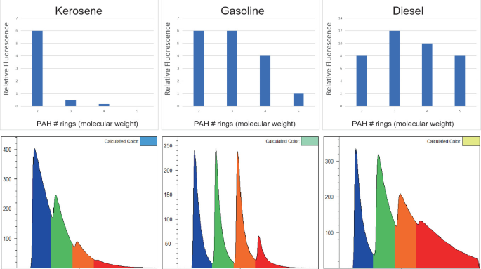

  

  NAPL fluorescence color dependence with PAH size and relative concentrations, and its effect on waveforms for common NAPL types

• 2. Waveform Intensity

• The y-axis on a waveform represents the intensity (brightness) of the fluorescence which is measured as a voltage generated by the photomultiplier tube detector which converts fluorescence flux to an electric current that is measured with a digital storage oscilloscope.

• The area under the curve of all four channels of the waveform is summed, divided by the area of all four channels for a reference emitter (RE) that was measured prior to logging.

• This normalization process allows the total fluorescence to be reported as a signal in %RE or total fluorescence of the LIF waveform versus the RE's waveform. The example waveform in Fig. 8.14 (right) had a strength of 203.6 %RE, so this diesel had about twice as bright total fluorescence intensity as the RE fluid measured prior to the diesel.

• For a homogeneous soil type and LNAPLs such as fuels, fluorescence is expected to increase monotonically with increasing concentration of fuels/oils in the soil pores. Figure 8.11 contains UVOST data obtained by measuring the fluorescence of diesel loaded onto moist coarse sand. Row three contains photos of those same sands (excited with a 308nm UVOST laser). Row four contains the resulting waveforms generated by each sample.

  Fig. 8.11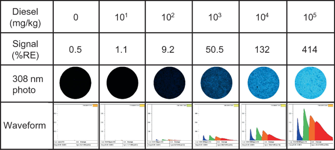

  

  Waveforms of diesel NAPL on 20–40 silica at decade concentration loadings

  Fig. 8.12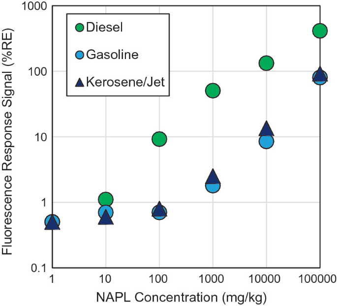

  

  Response of common NAPLs on 20–40 silica sand at decade series loadings

• Some fuel types fluoresce much more intensely than others. Diesel and crude fluoresce very well, while gasoline and kerosene (jet) fluoresce about 10–50% as intensely, as is depicted in Fig. 8.12, which shows the response for diesel, gasoline, and kerosene on UVOST.

• Porosity and grain sorting have a considerable influence on NAPL fluorescence (Alostaz et al. 2008) because coarse sediments allow neat NAPL pools to form up against the sapphire window and may even contain clear quartz grains whose transparency can increase the soil volume being interrogated. Fine-textured soils that assemble in a tightly organized matter more fully occupy the surface of the sapphire window and NAPL can hide in the soil’s complex structure.

• Figure 8.13 illustrates sediment type’s influence on fluorescence. Nine soils purchased as a kit from Midwest Geosciences Group (Indiana, USA) were loaded with 10,000 mg/kg (±100 mg/kg) of on-road diesel and 10% (±0.1%) of water, mixed well, left to rest 24 h, then examined under UV for homogeneity (proper mixing). Their fluorescence was measured, as well as clean sand at 10% moisture, using a UVOST system fitted with standard subsurface tooling. Figure 8.13 illustrates the dramatic difference in intensity due to sediment type alone (the clean sand/system background was 0.5% RE). Fortunately, NAPLs often distribute themselves within the more favorable soils in a geologic feature, if even the tiniest of pathways, and it is these NAPL-impacted seams and small pathways that the LIF responds to as the window slides past, if even for a brief moment. It should be mentioned that the waveform shapes (color and lifetimes) were essentially the same for each sediment, only their intensity (size) varied.

  Fig. 8.13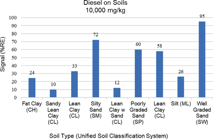

  

  UVOST response to diesel NAPL loaded at 10,000 mg/kg onto various soils (soils were pre-moistened to 10% water by weight)

• 3. Waveform Lifetimes

• The waveform’s x-axis spans 320 ns in time in order to capture NAPL’s brief fluorescence pulses.

• Fluorescence lifetime is defined as the length of time it takes for the pulse of fluorescence to decrease to ~ 1/3 (1/e) of its peak intensity.

• The LIF system’s software calculates the approximate lifetime and display them digitally.

• Notice that the lifetimes of some channels bleed into subsequent channels, which can influence the fill-colorization calculation—recent versions of LIF system software contribute the proper amount by using a relatively sophisticated allotment calculation.

• Long lifetimes often indicate ideal conditions, free from oxygen, with a solvent-rich fluorescence-friendly NAPL environment. Natural gas condensates, jet fuels, and diesels are ideal habitats for excited state PAHs and are known for their long lifetimes.

• Short lifetimes are indicative of excited state environments that are not friendly to excited state PAHs and one major cause is quenching by neighboring molecules that provide non-radiative pathways for excited state energy to leave the PAH, essentially snuffing out potential fluorescence before it can occur.

• Energy transfer causes a shortening of the lifetimes—the more closely packed the PAHs the greater the chance of energy transfer and quenching. This shortening begins to occur in heavy crude oils and gets steadily more extreme as the NAPLs get heavier (trending toward higher PAHs and less solvent) (Wang and Mullins 1994).

• Molecular oxygen, typically not present in situ at NAPL release sites due to anaerobic conditions, is a very efficient PAH excited state energy scavenger.

• Heavy NAPLs get spectacularly short lifetimes, even shorter lived than mineral fluorescence. This often allows for successful identification of heavies versus minerals.

• Heavies are immune to oxygen quenching due to their internal self-quenching which already quenches most susceptible PAHs regardless of molecular oxygen's presence.

8.6.4.1 Reference Emitter (RE)

Under normal circumstances, if one increases the excitation energy (the intensity of the laser light that is directed into the NAPL) one observes increasing fluorescence. Once excitation intensities get high enough however, the vast majority of PAHs are already driven into the excited state, so applying even more laser light intensity is fruitless. If we desire to consistently compare fluorescence data from one NAPL to another, or from one site to another, we can account for laser intensity variations in one of two ways:

• 1. Hold the intensity of laser excitation laser light delivered out the sapphire window to very consistent levels so that any changes in fluorescence can be attributed to the NAPL/soil matrix being measured, not to changes in the laser intensity.

• 2. Measure a fluorescent reference material’s fluorescence emission just prior to logging and normalize the subsequent in situ fluorescence readings by the response of this RE.

The first approach is difficult to achieve under laboratory conditions, let alone field conditions. So early on in the commercialization of LIF (Bujewski and Rutherford 1997), it was recognized that a stable fluorescent material, capable of fluorescing with consistency across the range of wavelengths typical of fuels and oils, be formulated and made available to practitioners of LIF. This proprietary blend of petroleum oils and stabilizers was dubbed “RE” and has been used for UV normalizing LIF data since the late 1990s and RE remains in use today. RE calibration is conducted in a fashion similar to the tank of 100 ppm isobutylene gas used to calibrate handheld PIDs. While PID responses are reported as the sample’s response relative to isobutylene’s response in “PPM”, LIF systems report total fluorescence intensity as a percentage of the RE’s total fluorescence flux called Signal (%RE).

Figure 8.14 shows the cuvette holder filled with RE fluid (top) and the RE’s waveform at left. The RE has a cross-section of 9992 pico-Volt-seconds (pVs) and a subsequently measured diesel on sand waveform (semi-transparent over RE’s at right) had a cross-section of 23,082 pVs. The resulting signal for this diesel on sand was thus 231.0%RE, a little over twice the total fluorescence intensity as the RE fluid.

Fig. 8.14

A cuvette filled with RE fluid held against the sapphire window of an LIF probe (top). The RE fluid’s waveform (bottom left) and the waveform produced by diesel on sand, with the RE waveform superimposed on top (bottom right)

Fig. 8.15

Waveforms of kerosene/jet fuel NAPLs on sandy soil. Row A is at equilibrium with room air’s oxygen, row B contains waveforms acquired after purging the NAPL of oxygen with nitrogen gas

The RE also serves functions beyond normalization for laser energy. Firstly, there is a desired instrumental range of fluoresce intensities, because if the RE response is too small (from insufficient laser light) then subsequent in situ fluorescence will also be too dim and electronic noise might interfere. If too much laser light is delivered, the fluorescence of even modest NAPL saturation would overwhelm the detection system (detector saturation would occur), reducing the upper NAPL saturation range of the instrument. LIF system operators adjust the laser intensity into the fiber so as to achieve an RE waveform that is of optimal intensity. The LIF software will not allow logging to proceed if the waveform is not within the proper range. Secondly, the LIF technician examines the relative response across the four channels of the waveform. If the ratio of the four channels relative to each other is not within the factory recommendations, the detection system needs to be adjusted to achieve the desired ratios. If not held within a few percent of their desired ratios, then subsequent waveforms acquired in situ of common recognizable NAPL types will not look familiar to data analysts. Imagine if one of the four channel were only 25% of the strength it typically exhibits. The result is that subsequent downhole encounters with NAPLs, even those of commonly recognized NAPLs, would be unrecognizable.

8.6.4.2 Waveforms of Common LNAPLs

Generally, similar fluorescence waveforms are emitted by families of fuels and oils with similar chemistries. This often allows LIF analysts to identify types of fuels and oils in situ, or at least whittle the possibilities down to one or two possibilities (Lu et al. 2014). But each fuel is a unique product depending greatly on the source crude and formulation, so even fuels of the same type do differ to some degree, sometimes surprisingly so, right out of the dispenser at the filling station.

Figure 8.15 contains waveforms of sandy material saturated with intact (unweathered) jet fuel and kerosene NAPLs. Notice the great dominance in the first channel, which is where naphthalenes fluoresce. Because the samples in row A were taken under ambient air conditions, molecular oxygen is present at ~ 20%, and molecular oxygen quenching is significant. The waveforms in row B are about twice as fluorescent and twice as long lived because the NAPL is relatively oxygen-free. Any benchtop studies of kerosene and jet fuel (measuring NAPLs recovered from wells for instance) should be interpreted with acknowledgment that the response is as much as a factor of two lower than what one will observe in situ because oxygen rapidly enters NAPL during normal handling in air. Interestingly, when kerosene weathers it does not red-shift to any significant degree like gasoline, rather its waveform retains the same shape and simply fades in intensity. This is because kerosenes contain insufficient numbers of PAHs of three or more rings to assume the task of fluorescing as the naphthalenes (and any other UV-fluorescing species) get preferentially washed out of the NAPL due to their higher semi-volatility and water solubility.

Figure 8.16 contains waveforms of three intact (fresh) gasoline NAPL saturated onto sandy soil at left. At far right is gasoline NAPL that had been saturated onto sandy soil and then allowed to weather indoors in a loosely lidded jar for seven years. Intact (unweathered) gasoline waveforms are typically shaped as shown, but exhibit variability due to their differing formulations. Oxygen quenching is a significant factor with gasoline as demonstrated by the two- to three-fold enhancement of both lifetimes and intensity observed in row B versus row A. Weathering has a significant impact on gasoline, demonstrated by the seven-year-old gasoline waveform at far right which is dramatically red-shifted. Notice, however, that oxygen quenching does not play a major role in the highly weathered sample. This is likely due to the reduction in gasoline NAPL volume, allowing energy transfer between PAHs to take place (a form of quenching) thus reducing oxygen’s contribution to quenching of PAHs within the sticky condensed coating of residual NAPL on the sand grains. There has been no clear indication that octane has much effect on fluorescence across hundreds of gasolines tested. However, premium blends appear less susceptible to weathering and have longer lifetimes in general versus lower octanes, due to differing formulation at the refinery.

Fig. 8.16

Waveforms of gasoline NAPLs on sandy soil

Figure 8.17 contains a sampling of diesel NAPL waveforms. Diesel has the unique characteristic of having a short lifetime blue peak (two-ring PAH UV emission) that is about the same height as the longer lifetime green peak, followed by three- to four-fold longer lifetimes in the subsequent channels. The reduction in oxygen quenching after removal (row B) is dramatic, with lifetimes so long that they look rather silly. How much of this is due to molecular dynamics versus detector saturation is unclear, but it makes many diesels instantly recognizable. Notice though how the diesel at far left has a waveform easily mistaken for gasoline, demonstrating there are often exceptions to the general waveform shapes of common fuel NAPLs. Evidence of weathering in diesels is not nearly as obvious as it is for gasolines, as is demonstrated in the waveform at far right which was weathered for seven years in the laboratory along with the gasoline discussed above. Notice there is reduction of the smaller more readily weathered PAHs (bluer channels) however, which is consistent with weathering of all NAPLs. Diesels have the longest lifetimes of all the commonly encountered NAPLs, with the possible exception of natural gas condensates. Notice also how the decay rate at the right side of channels three and four for de-oxygenated samples in the bottom row looks somewhat odd with a hump-backed appearance. This is likely due to interaction between PAHs via energy transfer, photon cycling that involves larger PAHs absorbing smaller PAH fluorescence and subsequently emitting fluorescence at longer wavelengths, or other complex interplay between PAHs for the excitation energy. These processes can take time and can be repeated, causing the unnatural upward bulge rather than the usual decay just after peak emission in latter channels.

Fig. 8.17

Waveforms of diesel NAPLs on sandy soil

8.6.4.3 Waveforms of Medium and Heavy NAPLs

Figure 8.18 contains UVOST waveforms of heavier unrefined NAPLs that are beginning to show the effects of having too many PAHs versus solvent molecules, which begin to affect their fluorescence. Energy transfer and photon cycling effects begin to have an ever larger impact as the NAPLs get heavier in molecular weight (PAH content) from left to right. Recall that these processes are lossy (often do not result in fluorescence), resulting in far less fluorescence than the NAPL’s robust PAH content would suggest. Dramatically shorter lifetimes are also the result when numerous larger PAHs are too close to the smaller PAHs that initially absorbed the UV laser excitation. This lifetime reduction gets steadily worse as NAPL density (relative PAH/solvent content) increases. These short lifetimes should be regarded as an obvious indication to the analyst that heavy NAPL may exist, and in great quantity, yet the heavy NAPL generates only a whisper of the signal %RE (relative to refined products that contain PAH/solvent ratios far friendlier to the fluorescence process). The reason we employ the word “may” above is because waveforms from false positives often display similar characteristics, making differentiation challenging. Identifying heavies and their relative saturation in soil with any UV-based fluorescence tool is fraught with the possibility of dismissing the heavies as harmless false positives or assigning harmless false positives as heavies. Heavy NAPLs should be investigated with TarGOST, the tool designed to respond appropriately to heavy NAPLs across a range of NAPL saturations.

Fig. 8.18

Waveforms of light crude, bunker fuel, creosote, and coal tar on sandy soil

• Crude oils respond well to UVOST LIF and as long as one is seeing modestly long lifetimes, such as the response in light crude (Fig. 8.18 far left), one can safely assume the relationship between Signal %RE and degree of NAPL saturation is likely to be monotonic, or at least nearly so. Light to medium crude waveforms are usually weighted slightly right of center (slightly red-shifted) on the waveform time axis and have modest duration lifetimes.

• The fill colors in the upper right corner of the waveforms in Fig 8.18 are all fading orange to red, this is another visual clue of the presence of heavier (or extremely weathered) NAPLs in a UVOST log, which will have their Signal %RE plot filled with red indicating zones where heavies (or false positives) are encountered.

• Because their chemistry spans the transition from relatively ideal fluorescence behavior to extreme energy transfer effects (Wang and Mullins 1994), crude oils also spectacular variety of waveforms, depending greatly on their source and chemistry. They can be relatively blue-shifted and long-lived or tremendously red-shifted and short-lived, making crudes difficult to identify definitively as crude with LIF data alone.

• Crudes contain not only fluorophores, but chromophores as well, which are molecules that absorb wavelengths of light involved in LIF processes but do not fluoresce, so chromophores can cause significant quenching in crudes and other heavies.

• The fluorescence of NAPLs heavier than light crudes also begins to exhibit fluorescence intensity behavior that does not scale properly (monotonically) with the degree of NAPL pore saturation. Most heavy NAPLs will be grossly under-reported by any UV-excitation fluorescence system.

• Bunker fuel (second from left) is heavier in average molecular weight than light crude, higher in relative PAH content and contains less VOC solvents, so energy transfer red-shifts the color, lifetimes begin to shorten, and precipitous drop in total fluorescence occurs. UVOST is capable of absence/presence of bunker, but false positive interference and almost certain lack of monotonic behavior begins to complicate interpretation and limit utility of the data.

• Creosote (second from right) is in the same category of fluorescence as bunker fuels in that they often fluoresce at the same intensity across a wide range of NAPL saturation. From 100 ppm, all the way up to full saturation, they can yield approximately the same %RE response. While completely missing creosote is unlikely for UVOST, the logs at creosote sites give little indication of the relative NAPL content in the soil, only absence/presence.

• Coal tar (far right) is the most concentrated PAH NAPL encountered with LIF, with PAHs sometimes occupying over 50% by weight. This oversaturation of PAHs is instantly recognized in the coal tar waveform, which has the shortest lifetimes of any NAPL, combined with a fluorescence intensity that is also extremely low and sometimes not exceeding the natural soil’s response. Coal tars can still hint that they are present however, by a red-shifting and short lifetime waveform even more extreme than soils or other false positives, but it takes a keen eye and discipline to spot them, especially if their presence is unexpected at the site.

8.6.4.4 Waveforms of False Positives

Soils can generate fluorescence that does not originate from the NAPLs being targeted. These non-NAPL positive responses range from weakly fluorescing to strong and even dominating fluorescence (higher than target NAPL at full saturation). Sources include organic materials such as phragmites roots, meadow mat, certain clays, calcareous sands, buried woody debris, or even aqueous phase PAHs associated with nearby heavy NAPLs like coal tar. Almost any man-made non-metallic materials fluoresce (concrete slurry, paper, sewage, biodiesel, plastic, fabrics, etc.) so investigators should always be on the watch-out for waveforms that do not match the fuels/oils on site, especially shallow. Figure 8.19 contains a sampling of typical false positives encountered during UVOST logging.

Fig. 8.19

Waveforms of commonly encountered false positives

Aspects to keep in mind about false positives include:

• Fluorescence intensity from false positives is sometimes not that high (< 5%RE), but those levels can actually be quite problematic when they occur in and among weakly fluorescing NAPL (e.g., gasoline) seams or weeps of NAPL found in small grained soils which creates NAPL and soil combinations that are not strongly fluorescing themselves.

• Almost all false positive soil waveforms differ from NAPLs due to their short lifetimes and the “trident spear” shape in the last three channels. This makes recognition of NAPL in and among these common false positives, and subsequent rejection of false positives from the NAPL CSM, possible and even routine.

• Clays (far left in Fig 8.19) often fluoresce in the few percent RE range. They can be confused for heavies and limited targeted sampling is often required to establish the true origins of this waveform.

• Calcareous sands (second from left) are common along coastal environments and can sometimes yield strong fluorescence signals. Probing in constantly fluorescing soils seems like an impossible environment to sensitively detect NAPL fluorescence in, but the longer lifetimes exhibited by LNAPLs typically make discernment of NAPL relatively easy to discern from fluorescing sand.

• Peat (second from right) is highly variable in its fluorescence, ranging from none to as high as 50%RE. Finding heavy NAPL contamination in peat lenses is one of the most challenging scenarios for LIF.

• Any living or recently decayed vegetation will exhibit fluorescence, but it is typically limited to a few %RE intensity and recognizable as non-NAPL in nature due to the familiar “trident spear” waveform. Aquatic vegetation false positives are commonly encountered at the sediment surface during offshore barge-mounted LIF projects on canals, rivers, and other water bodies adjacent to onshore NAPL release sources.

• The only long-lived “blue-dominant” false positive waveforms encountered in the 30 years of LIF have been volcanic soils in the Aleutian Islands and these fluoresced in the 0–3%RE range.

• One should always budget for modest level of targeted sampling from LIF locations and depths where potential false positives exist to determine what materials are causing unfamiliar fluorescence waveforms and their fluorescence must be removed from the data set if they are found not to be target NAPL.

Fig. 8.20

Coal tar and aqueous phase PAHs in a jar at left accompanied by their inverse responses to UVOST LIF when saturated onto sand at right

An extremely problematic type of false positive mentioned previously is aqueous phase PAHs that occur in sandy or gravelly soils in the immediate vicinity of heavy NAPLs such as coal tar. The reason it is rare is that probing in/near very heavy NAPLs with UV is avoided by reputable LIF providers, who recognize the danger of misidentifying dissolved phase as LNAPL and subsequently reporting them as such. Figure 8.20 contains a benchtop demonstration of the danger of probing coal tar with UV fluorescence. The jar (A) contains coal tar and water and the tar is stuck to the jar’s sides and bottom with a layer of water between the NAPL. After some time (days to weeks), the PAH-rich tar sources smaller more soluble PAHs to the water and these smaller two- to three-ring PAHs are readily excited by UVOST’s UV laser. Because the larger PAHs are practically insoluble in water, there are not enough of them to promote energy transfer and its associated quenching. This leaves the smaller aqueous phase PAHs to fluoresce unencumbered, as demonstrated by the sky blue fluorescence in the jar (B). They fluoresce so well, in fact, that when this same water is used to saturated sand, its fluorescent waveform mimics partially saturated gasoline NAPL (4.2% RE) and would almost certainly be interpreted as such (D) by the analyst. The waveform of the source coal tar meanwhile (C) at total saturation on sand, yields a factor of seven lower response (only 0.6%RE) which is easily dismissed as insignificant (false positive), especially by inexperienced data analysts.

LNAPLs do not suffer from this aqueous phase PAH false positive because the LNAPL solvent body is quite capable of hosting hydrophobic PAHs. Heavy NAPLs on the other hand are at or near saturation with PAHs and the tremendous concentration gradient between the DNAPL and water is high enough to generate high dissolve phase PAHs (compared to waters adjacent to LNAPLs). Waters adjacent to LNAPLs do of course contain dissolved PAHs, but at a concentration too low to rival that of their LNAPL source NAPL when that water is loaded onto soil.

8.6.4.5 Weathering Effects on LIF Response

Weathering selectively removes the most soluble, most volatile, and most readily metabolized hydrocarbons first (including PAHs), which means the smaller PAHs are the first to go. This process selects an ever larger size population of the PAHs who continue to reside in the remaining NAPL. And because the larger remaining PAHs fluoresce in redder colors, weathering causes a red-shift in waveform color. At the same time, the loss of the NAPL “solvent body” (including the BTEX and aliphatic fluids that help solvate PAHs) makes for a less fluorescence-friendly liquid hydrocarbon environment. This loss of solvate often shortens the lifetime, so combined with the color shift, a weathered lighter fuel’s waveform will begin to mimic heavier NAPLs, and eventually look more like an oil or even a tar than the original LNAPL. This makes sense to us because weathering processes are slowly converting the lighter LNAPL to a heavier NAPL, which in its final extreme stages contains only the large and “sticky” molecules that are the hallmark of heavy NAPLs.

Because the average molecular weight of gasoline is relatively light, it contains many volatile and relatively soluble molecules, making gasoline particularly susceptible to weathering. A simple but effective method for emulating mechanical weathering of gasoline is to introduce nitrogen gas at 300 ml/minute into a vial containing ~ 5 g of 87 octane gasoline saturated onto moist sand (10% water). Logging the UVOST LIF response continuously as the nitrogen flows allows one to observe the waveform changes that occur due to the chemical makeup changes over time. Figure 8.21 contains the UVOST waveforms taken over time, from pre-flow of nitrogen (air equilibrium) to 20 min after flow was begun (20 min N₂ flow). The voltage scale on the four waveforms is scaled independently to allow us to closely observe the color and lifetime changes, hiding the fact that they were not all the same height (voltage).

Fig. 8.21

Artificial weathering of gasoline via nitrogen gas flow

At air equilibrium, the waveform was heavily quenched by room air's 20% molecular oxygen, as evidenced by the short lifetimes and low %RE. Whatever PAHs were responsible for the fluorescence in channel two (green channel), they were particularly susceptible to having their excited state energy stolen by molecular oxygen. Just one minute after starting the flow of nitrogen, the bulk of the oxygen has been removed and both the lifetimes and intensity increased dramatically for this particular gasoline formulation. Removal of the most volatile of the PAHs (responsible for the blue, UV channel) was already being reduced at this point. Six minutes after flow started, continuing selective removal of both the more volatile PAHs and solvent body VOCs continued to red-shift the fluorescence and shorten the lifetimes. After 20 minutes of flow, the gasoline fluorescence has transformed markedly from its original (intact) fluorescence. This virtual rainbow of responses is commonly observed at gasoline release sites and helps reveal insights into the condition of gasoline NAPL with depth.

Mechanically weathering gasoline at such a rapid pace is of course a much faster process than that occurring in situ, but it serves as a convincing demonstration of the fluorescence red-shifting that weathering causes. Remember that jet/kerosene weathering is typically indicated by decreasing fluorescence but no color shift because there is an insufficient number of larger PAHs left to continue the fluorescing once the semi-volatile naphthalenes have been weathered out. In general, the heavier (and therefore more recalcitrant) a NAPL is, the less its fluorescence response changes with weathering.

8.6.4.6 Cluster Diagrams

As we have just seen, waveforms are a compact way of envisioning all main fluorescence properties, but their vast numbers make them difficult to comprehend site-wide. What was lacking for quite some time in LIF’s history was a method of reducing waveforms down to a more compact form, where each and every waveform’s contribution to the log could be visualized in one graphic, and this lead to the development of the cluster diagram.

Cluster diagrams begin with a waveform reduction process to each of the waveforms in a log, breaking every waveform down into its four individual fluorescence decays. The top row of Fig. 8.22 shows a waveform of typical fuels (kerosene, gasoline, and diesel) that have undergone the data reduction processing with individual decays shown after process along with waveform in black outline. The gasoline waveform (top center) shows the four channels’ intensity factors (black arrows) and the four lifetimes (orange arrows) that were determined during the processing for that waveform. The four relative strengths represent relative color, so their relative left–right balance is used to calculate each waveform’s bubble and their position in the color axis (x-axis). In this fashion, very blue-shifted waveforms like kerosene land at far left of the cluster diagram and very red-shifted NAPLs (highly weathered or heavy NAPLs) land very far to the right.

Fig. 8.22

Top: Three common fuel class waveforms reduced to independent decays. Bottom: cluster diagrams of artificial weathering for six kerosenes/jet fuels (left), ten gasolines (center), and six diesels (right)

The average of each waveform’s four channel lifetimes is used to determine where on the lifetime axis (y-axis) of the cluster diagram each waveform’s bubble should be placed. The cluster data are normalized to place very short lifetimes of < 1 ns (like coal tar or soil fluorescence) toward the bottom, and long lifetimes like that of diesel near the top. Each waveform is thus transformed into a bubble that occupies its own unique position on the cluster diagram “map”, with its position describing the color and lifetimes contained in the original waveform. The fluorescence intensity of the total fluorescence (%RE) is portrayed by sizing each waveform’s bubble according to its signal %RE, up to a capping level that changes with each LIF family.

Figure 8.22 bottom row contains cluster diagrams for UVOST logs gathered during weathering studies of six kerosenes (left), ten gasolines (center), and six diesels (right). Cluster plots of weathering experiments for a number of the same fuel types serves to illustrate where the certain fuel type’s bubbles land on the clustering diagram, as well as how individual chemical formulation differences and weathering affects their positions. The samples were flushed with a gentle stream of nitrogen gas to displace oxygen and left to flow over a 20-min period. The changes in molecular oxygen content (and subsequent degree of quenching) combined with selective weathering of smaller semi-VOCs resulted in continuous “tracks” of bubbles for each NAPL species, each track representing shifts in color and lifetime that occurred in the fluorescence during this artificial weathering process. Recall that oxygen’s presence shortens the lifetimes and this is evident in the bubbles circled in blue, showing the cluster positions for waveforms acquired while the fuels still contained oxygen. In the gasoline cluster (center), bubbles rose sharply on the lifetime axis during the initial oxygen removal (a process taking less than a minute to complete) and then lifetimes trend steadily downward again within the 20-min nitrogen flow that is causing mechanical weathering of semi-VOCs and the VOC solvent body. Notice also how the gasolines’ bubbles spread to the right in color (red-shifting) as discussed in the previous section.

The gasoline samples’ bubbles are cast across a wide range of both fluorescence color and lifetimes, while diesel and kerosene are more stable with regard to color shifts, creating tighter clusters, but shifted up and down by oxygen quenching effects. This same “vertical stacking” pattern for diesel is often observed for diesel NAPL located near the soil surface, where oxygen and weathering have the most influence due to earth tides. The general trend is that cluster bubbles for all LNAPLs generally head to the right (red-shift color) and down (shorter lifetimes) as the degree of weathering increases, but effect is most pronounced in gasolines because they vary most with original formulation at the refinery and with weathering. Figure 8.23 contains a UVOST cluster diagram map, with regions where fluorescence responses for various fuel classes reside highlighted. There is modest overlap between the different fuel classes, indicating that LIF data is definitive in some cases, but variations in NAPL chemistries due to source and weathering can create less than certain waveform interpretation in many instances.

Fig. 8.23

UVOST LIF cluster diagram showing the regions occupied by common NAPLs and false positives

8.6.5 Analysis and Interpretation of LIF Logs

8.6.5.1 LIF Logging in Practice

Over the last 30 years, the most common log interpretation mistake, by far, has been to focus solely on fluorescence intensity, without tempering the intensity-focused interpretation with the other valuable information contained in the log. Intensity alone simply cannot be trusted to represent the NAPL in situ, due to highly variable fluorescence intensity from NAPL to NAPL, weathering, and false positives sometimes out-fluorescing the NAPL, so adjusting our interpretation by including the color and lifetime in the analysis is a key part of LIF log interpretation.

Log interpretation will be now be demonstrated based on the same idealized scenario employed to illustrate the application of HDCS and MIP (Figs. 8.2 and 8.4, respectively), which will be assumed to be contaminated with gasoline NAPL (Fig. 8.24).

Fig. 8.24

Idealized scenario of gasoline NAPL in the soil column at left and resulting LIF (UVOST) data at right

In Fig. 8.24, the Signal %RE x-axis approximately covers the range 0–150 %RE which most gasolines typically produce. Gasoline NAPL is complex in its fluorescence due to its propensity for weathering rapidly and more extremely than other commonly delineated petroleum NAPLs. The Visible Fluorescence column in Fig. 8.24 illustrates this, showing us how gasoline behaves like a chameleon with regard to its fluorescence color. Depending on the source and age it varies wildly, occasionally fluorescing nearly as blue (UV) as kerosene, while premium gasoline can come close to mimicking diesels. Weathering can cause red-shifting that generates waveforms that mimic light to medium crudes. Every gasoline release site’s fluorescence looks different because every site has a unique history of gasoline formulations released, age and weathering processes. Figuring out the details of exactly what, when, and how past NAPL releases occurred is always difficult, but an LIF survey provides, at a minimum, an immensely useful guide to where gasoline NAPL is and insights into the chemical nature of the NAPL at thousands of data points in the subsurface.

Key observations for the gasoline NAPL profile in Fig. 8.24 include:

• Interval A

The NAPL is perched near the surface, leaving it more vulnerable to aerobic and physical weathering, so the intensity is somewhat lower than it would be had the NAPL not been weathered. More dramatic signs of weathering are recognizable in the Visible Fluorescence column showing a turquoise color which is red-shifted from the deep blue–violet color typically exhibited by intact gasolines. The callout waveform here is classic highly weathered gasoline (which looks similar to light crude). The lifetimes are modestly short, consistent with gasoline that is weathered and may be exposed to oxygen. Notice that the signal fill color here is orange, so we might be tempted to call this false positive fluorescence, but the lifetimes are still long enough (noticeably up off the natural soil baseline) to assure us this is NAPL.

• Interval B

Despite the presence of VOCs, LIF fails to register any Signal (%RE) response above background because LIF is not capable of detecting gaseous, aqueous dissolved or sorbed VOCs like a MIP can.

• Interval C

The “shark’s fin” shaped profile in the Signal %RE replicates the idealized Gasoline NAPL saturation profile nicely, but a close inspection sees color shifts occurring across this profile. The very top of the shark’s fin exhibits several signs of weathering including the turquoise color in Visible Fluorescence, and both the lifetime and Signal %RE increases do not increase in concert with the gasoline NAPL saturation. Once down into the higher saturation of the gasoline NAPL, we return to a classic intact gasoline waveform with robust UV contribution in the 350 nm (blue) channel of the waveform, and the modestly long lifetimes that intact gasolines usually exhibit. The cobalt blue in the Visible Fluorescence is typical of intact gasoline’s blue, indigo, and violet emission that human eyes can just barely see. This is rendered as a chartreuse signal fill color in the OST software, which is a fill color commonly generated for intact gasolines.

• Interval D

The orange fill color in the Signal %RE response here hints that it is very likely soil fluorescence. Due to the nature of this being a gasoline release (which we know from the waveforms above and below), there is a heightened chance that Interval D actually represents a thin lens of extremely weathered gasoline. However, there is a lack of increase in the lifetime column, indicating that it is unlikely to be extremely weathered gasoline and is instead mineral in nature (false positive). Either interpretation of this interval is low risk (compared to the more robust and confident NAPL intervals).

• Interval E

Notice how the chartreuse signal %RE fill color on top side of the Signal %RE response fades to orange at the bottom. Like Interval C, this trapped lens of gasoline shows signs of weathering, but in reverse. This interval’s more weathered gasoline NAPL is located where groundwater dissolution is taking place along the NAPL body's bottom edge. The more intact gasoline NAPL in Interval E is that which is held up against the low-k clay that protects this NAPL deposit from weathering. The lifetimes support this as well, shortening in concert with the red-shifting of color due to weathering.

8.6.5.2 Field Logs

For purposes of providing a single comprehensive field log, Fig. 8.25 was created by stitching together three different UVOST field logs obtained at three NAPL release sites in the USA in 2018–2019. The potentiometric surface elevation indicated in this profile (at 10 m below ground level) truly was co-located in relation to the NAPL data shown in that same interval C.

Fig. 8.25

Top: Composite UVOST field log containing typical responses for gasoline, diesel, false positive soils, and kerosene

Prior to discussing the fluorescence of this field log, let us introduce several elements of LIF field logs not yet covered. At left are the callouts, each numbered 1–5 in their upper corner. Each waveform has information below it describing the depth and signal %RE for that waveform. Callouts 2 and 5 were single waveforms, while callouts 1, 3, and 4 were selected from a range of depths, so they contain the average of all waveforms that were acquired between those depths.

The cluster diagram for this log’s waveforms is at far upper right. Small tags with the callout numbers are made next to bubbles representing the waveforms and, in the case of range callouts, a polygon roughly encircling those bubbles represented in the range. Next to the cluster in the vertical log section, you see the X: Wavelength column that contains each waveform bubble’s x-axis cluster diagram position (A-J). Alongside, it is the Y: Lifetime log that indicates each waveform bubbles’ y-axis position (0–10) on the cluster diagram. This allows for high definition examination of both color shifts and lifetime at all depths.

• Interval A

This first encounter of significant fluorescence is not a cartoonish hump like those used in the simplistic training models (Fig. 8.24). NAPL fluorescence is often observed as a bristly pattern of high and low fluorescence encounters which are accurately mimicking the highly heterogeneous NAPL distribution commonly observed in situ.

A core from this interval would yield discrete patchy mottling or distinct lamina of gasoline NAPL-impacted soils sandwiched between soils that contain little or no NAPL (or fine soils such as clay that partially hide the fluorescence). This insight into the existence of small-scale extremes in distribution is another aspect of LIF logs that often goes underappreciated but can be valuable for those considering potential NAPL recovery, NAPL transmissivity (García-Rincón et al. 2020), and associated remediation system design.

The presence of gasoline far above the water table may suggest a release source is perhaps nearby (some gasoline perched during its fall through the profile) and that the gasoline is perhaps sitting above a capillary barrier.

• Interval B

This interval contains what at first glance appears to be a trivially small Signal %RE. But absent evidence to the contrary, one can never rely on intensity alone to conclude a response is insignificant. Examination of the waveform, fill color, and lifetime suggest interval B is either a harmless false positive soil or organic. But a much more consequential interpretation is that it is instead a heavy NAPL such as coal tar which would yield a similarly red-shifted signal. We simply cannot rule this possibility out, so this interval should be validated at least once at this site or further assessed considering the site history and other site characteristics (e.g., the presence of fluorescing kaolinite or montmorillonite).

• Interval C

This NAPL is distributed in a shark’s fin fashion poised on the water table. The waveforms, calculated fill color, long lifetime, and high center-right location on the cluster diagram all point to an intact diesel. A lens of low hydraulic conductivity soils probably exists at ~10.1 meters, causing the brief “cut out” in the Signal %RE response of this otherwise classic shark’s fin profile that is typical of NAPL residing on groundwater surfaces in transmissive soils. Careful examination of the calculated fill color along with X: Wavelength and Y: Lifetime columns, indicates that there is weathering at the bottom of the fin, and those weathered NAPL responses are represented by the green to light orange bubbles in coordinates F4, F5, G5, G6, G7 of the cluster diagram. This is the vertical stacking behavior, a weathering behavior that is commonly observed with diesel (see Fig. 8.22 lower right).

One might be tempted to assume that the NAPL in interval C contains far more saturated NAPL than other intervals, and is therefore more consequential to the NAPL CSM than intervals A or D, but that is not necessarily true. This is another common interpretation error, that is, not considering the inherent fluorescence intensity differences between NAPL types and varying sediment types. Because gasoline is considered to have higher risk for sourcing BTEX, interval A might well be of more interest to stakeholders than interval C and in fact the gasoline in interval A could have saturation levels matching that of the diesel in interval C.

• Interval D

Interval D is trapped well below the water table, which is not uncommon due to water table fluctuations. Interval D’s fluorescence is extremely blue-shifted, long-lived, and its waveform is consistent with kerosene. Callout tag 5 of the cluster diagram shows it is located in the extreme upper left, where no other common NAPL types are found with the exception of some natural gas condensate formulations. The few signs of weathering are at the top and bottom of this NAPL lens, and those waveforms are stringing down toward the bottom right of the cluster (coordinates B8, B7, and C6), consistent with weathering of NAPLs that drives them in this downward and slightly right (red) direction.

If one desires to do site-specific calibration studies in order to convert signal %RE to NAPL saturation or similar metric, spiking NAPL recovered from the site onto representative site soils in a decade dilution series (as was done to generate Fig. 8.12) will get one closest to realistic conversion from Signal %RE to estimated NAPL saturation.

8.6.5.3 Non-negative Least Squares (NNLS) Fitting

Our final topic with regard to fully utilizing the qualitative aspects of fluorescence inherent in an LIF data set’s waveforms, involves processing the thousands of waveforms gathered across a NAPL release site through non-negative least squares (NNLS) fitting or similar techniques in order to infer, continuously with depth, where different NAPL types and/or false positives are found. This is typically conducted after all types of fluorescence observed at the site have been somehow vetted, leaving us confident that we know enough to determine what fluorescence we want to keep (target response) versus those type of fluorescence we would like to discard or otherwise ignore.

The waveforms that represent the main classes of fluorescence observed in the log (or entire site) are called the basis set, a collection of up to five waveforms in the current OST software. The basis set created for our composite log is shown in Fig. 8.26.

Fig. 8.26

Basis set of waveforms for NNLS processing of the composite log

The processing involves application of a NNLS fitting algorithm to determine which waveforms in the basis set, and how much contribution of each waveform, need to be combined in order to generate a synthetic waveform that best fits every in situ waveform in the log. The result contains a separate log for each basis set waveform (fluorescence type), representing how much (in %RE) each basis set waveform contributed to achieve the best fit. Figure 8.27 contains the results for our composite study log. The signal scale is held to 25 %RE to allow us to see the results for all types of fluorescence, including the weaker ones (resulting in some NAPL types plotting off-scale to the right). Notice how the NNLS process successfully isolated each basis set fluorescence type according to where it was observed, with the exception of highly weathered diesel at 12–13 m below ground level, where the NNLS process chose mostly weathered gasoline instead. This was because weathered diesel was not available in the basis set and highly weathered gasoline and highly weathered diesel color and lifetime begin to converge, so NNLS chose the closest match in its basis set to fit the weathered diesel.

Fig. 8.27

The composite log at left along with the resulting basis set logs, each containing their contribution to the total fluorescence signal (in %RE) with depth

NNLS processing is often applied to an entire set of LIF logs from one site characterization effort, which often contains dozens to hundreds of logs. These logs contain many thousands of waveforms, all from unique points in 3D space. NNLS processing enables stakeholders to separate mixed NAPL bodies up into their respective NAPL types, eliminate false positives from target NAPLs, and other complex situations. Figure 8.28 contains the fluorescent response of a mixed NAPL body at a gasoline filling station site that was separated into fluorescence types (corresponding to intact gasoline, weathered gasoline, and diesel) using NNLS processing (ITRC 2019).

Fig. 8.28

3D visualization of a mixed NAPL body broken up into separate bodies using NNLS processing. Green corresponds to “weathered gasoline”, blue to “intact gasoline”, and yellow to “diesel”

8.6.5.4 Validation Sampling of LIF

Targeted validation of LIF logs with co-located core sampling is invaluable, but can also be misleading unless one is prepared to manage the effects of NAPL's often extremely heterogeneous distribution. Comparisons between LIF logs and physical samples taken adjacent to NAPL indications in LIF logs often show poor correlation, with the primary cause being localized heterogeneity. The simple act of acquiring samples from a separate adjacent borehole can result in mysterious depth offsets due to compression, partial recovery, and human errors. The key to conducting valid comparisons between the two is to implement controls by comparing multiple lines of evidence of the soil subsamples from the cores with benchtop LIF of those very same subsample intervals.

Figure 8.29 contains a “data dashboard” style assembly of data from validation of a fairly typical UVOST log that was acquired at a gasoline NAPL release site. Validation of this particular field log was requested by the client, so a core was retrieved from the same depth interval as the LIF log response using a direct-push sampler. The core was taken less than one meter away from the in situ UVOST log. Recovery was nearly 100%, the core was capped, shipped unfrozen to the LIF provider, frozen for 24 h, split open with a masonry saw and the exposed soil surface was scraped clean. The clean face was screened continuously with UVOST by sliding the sapphire window sensor along the core's face, the core was photographed in visible and UV lamp light, then sprayed with a proprietary NAPL indicator dye, and photographed under UV again. The in situ log is at far left of Fig. 8.29, the benchtop UVOST log is at center, and core photos are located at right. Hanging the multiple lines of evidence in a vertical fashion makes analysis a lot easier for most than staring at spreadsheets of data.

Fig. 8.29

Validation of a UVOST log with benchtop UVOST, photography, and emulated NAPL validation at narrow intervals

The first thing one notices in Fig. 8.29 is that the in situ LIF log at left is noticeably different than the ex situ LIF log adjacent to it. The NAPL in the in situ log appeared to be one half meter of depth deeper than the ex situ log’s NAPL response. The cause for this depth mismatch is, as usual, a mystery. It could have been human error, NAPL heterogeneity in the soil, direct-push rod flex, or some combination. In addition, the ex situ LIF result is lower signal with more weathered looking (red-shifted) waveforms compared to in situ response. This difference is consistent with our experience for benchtop validation works, especially in the case of gasolines. The difference is likely due to both molecular oxygen quenching and sample handling induced weathering affecting the ex-situ LIF response.

The ex-situ LIF responses match up almost seamlessly with the fluoresce photography and dye testing. Only by conducting such “apples to apples” analyses on narrow intervals, with multiple NAPL-sensitive methods, are were able to successfully control for NAPL heterogeneity and/or any human or mechanical error. Notice how poorly the downhole data (green diamonds) correlates with all the other lines of evidence. This is because the green diamond data points were gathered from different soils than all the other lines of evidence. All other lines of evidence were gathered from the exact same soils, thus the up-hole data have good correlation.

8.7 Tar-Specific Green Optical Screening Tool (TarGOST^®)

In the UVOST discussion so far, we described the alarmingly low response generated by heavy (dense) NAPLs such as coal tars, creosotes, and bunker fuels. At best, UV-induced fluorescence intensity of heavies rises a bit at low NAPL saturations but then plateaus, showing no additional response with increasing saturation. At their worst the fluorescence response of heavies begin to decrease as NAPL saturation increases, making UV-induced fluorescence unsuitable for screening for heavies due to the high risk of false negatives. This low fluorescence response might be tolerable if it were not for false positive fluorescence emitted by organic and soils, which normally contribute only a subdued fluorescence relative to the brightly fluorescing lighter NAPLs such as refined fuels. But false positives are often able to emit enough fluorescence to make total fluorescence intensity alone a poor indicator of their presence. And in some case, the false positives fluoresce just as brightly, if not brighter, than heavy NAPLs, making it nearly impossible to screen for heavy NAPLs without grossly exaggerating their footprint. Finally, there is also the fatal flaw of the fluorescence of aqueous phase 2–3 ring PAHs that often reach high concentrations in pore waters adjacent to heavy NAPL (Fig. 8.20) and are easily mistaken for an LNAPL by UV-induced fluorescence sensors.

The TarGOST form of LIF was introduced in 2004 as a solution to these issues and was rigorously vetted for use on coal tar NAPLs at former manufactured gas plants (MGPs) (Coleman et al. 2006). TarGOST differs from UVOST in that it responds monotonically to the vast majority of heavy NAPLs. TarGOST waveforms also more capably discern differences between heavy NAPL chemistries and the false positives of organic materials that so often exist in quantity at wood treater (creosote) and former MGP sites (due to being built alongside water bodies). TarGOST is virtually unresponsive to dissolved phase PAH fluorescence, eliminating the risk that this false positive introduces to UV-induced fluorescence. One very rare exception are acid tars, which can source acid form (water soluble) PAHs to groundwater which TarGOST can respond to.

TarGOST’s waveform callouts, cluster diagrams, and associated reporting are similar to that previously discussed. The excitation and fluorescence emission wavelengths were simply shifted to lower energies (longer wavelengths). This was done to specifically target directly the exceptionally large PAHs that dominate the fluorescence of heavies thus passing over to, some extent, the energy transfer quenching observed with UV-excitation fluorescence.

Heavy NAPLs are often DNAPLs, so the herding effect that gravity and LNAPL’s buoyancy have on driving LNAPLs toward the groundwater’s potentiometric surface does not apply to them. This causes heavies like coal tars to sink and crawl laterally, distributing themselves even more heterogeneously than LNAPLs. Compound this with the fact that heavy NAPL sites have had up to a century for the released NAPL to distribute themselves, and the architecture of DNAPL bodies is inevitably more complicated and chaotic than that of LNAPLs. There are occasionally very large and important sites, where addressing the nature and extent of any and all petroleum LNAPLs, coal tar and creosote (DNAPLs) in one logging event is considered critical and worth the extra expense. Dual-windowed subs are available for such occasions which allow both UVOST and TarGOST to occur simultaneously in the same logging event (Tomlinson et al. 2017). Dual LIF logging assures that any NAPL encountered will have at least one LIF system capable of responding monotonically, almost foolproof recognition of NAPL type and improved identification of false positives.

Figure 8.30 contains a fairly typical TarGOST log. Log interpretation remains much the same as for UVOST logs but with some key differences. One difference is the introduction of an excitation laser scatter channel, which replaces the left-most fluorescence channel, leaving the last three channels of the waveform to represent fluorescence. The laser scatter (A) and fluorescence (B) channels are processed separately and displayed in their own columns. Signal %RE (C) is calculated using a proprietary method that results in a response that scales monotonically with the presence of heavy NAPLs. Note that UVOST and TarGOST use different RE substances, so there is not a direct relationship in %RE values across TarGOST versus UVOST.

Fig. 8.30

TarGOST log consisting of former MGP coal tar NAPL in callouts 2 and 4, with a layer of woody debris in callout 3

The cluster diagram bubble positions for TarGOST logs are based only on the three fluorescence channels (at right in the waveforms) to characterize the fluorescence colors and lifetimes as is done with UVOST's four channels. Bluer colors (lighter NAPLs) plot on the left of the x-axis and redder colors (heavier NAPLs) on the right, with average lifetimes plotted on the y-axis. Heavy NAPL fluorescence lifetimes observed with TarGOST are never as long-lived as UVOST LNAPL fluorescence, so the lifetime axis of the cluster is far more sensitive to even minor lifetime shifts than the UVOST cluster diagram. Contained in both the upper and lower intervals (D) of the log in Fig. 8.30 is the coal tar DNAPL that was being targeted for characterization. The turquoise response in interval E was immediately recognized as not matching the known coal tar waveform, so that interval was sampled and found to be a layer of woody debris.

It is important to recognize that interpretation of this log based on the fluorescence intensity alone (column B) is folly because the false positive (wood) is dwarfing the coal tar NAPL’s fluorescence. This is a common occurrence at wood treater and former MGP sites. In this particular case, lifetimes alone did not serve as a sufficient aid for differentiation of the two, but the fluorescence color combined with the lifetimes of the two were quite different. In other cases, the fluorescence color of target NAPL and false positive are identical, but lifetime differences allow for their differentiation and successful data filtering via NNLS techniques. In the rare cases (well over 500 sites have been investigated with TarGOST to date) that significant false positive organics and the target NAPL fluoresce are identical in both color and lifetime, interpretation of the TarGOST logs is limited in its specificity, which dramatically reduces our confidence in the LIF site model’s veracity. It is difficult to overstate how often fluorescence of heavy NAPLs and natural organics are encountered at the same site and need to be separated from each other. In fact, it is more often the rule than the exception. This issue is effectively dealt with by applying NNLS fitting and other approaches (St. Germain 2011), but it is something that will almost certainly occur, so it is important that one budgets for some limited validation and processing, and work closely with your service provider to stay alert for its inevitable occurrence.

Because heavy NAPLs have such a high PAH to solvent NAPL ratio, self-quenching of fluorescence between PAHs is significant, causing generally short lifetimes in all heavy NAPLs. Molecular oxygen quenching of NAPL, a major influencer in benchtop UV-induced fluorescence measurements of LNAPLs discussed previously, has not been observed to be an issue for benchtop TarGOST fluorescence measurements of heavy NAPLs. In addition, weathering-induced loss of PAHs appears to have a negligible effect on the fluorescence color or lifetimes of heavies, because it is likely that there is such a surplus of PAHs of all sizes, that weathering’s minor effects are not noticeable with regard to fluorescence.

TarGOST waveforms are capable of general discernment between NAPL classes, in a manner similar to UVOST. Figure 8.31 depicts cluster diagram bubbles from a suite of medium to heavy NAPLs, along with their waveforms.

Fig. 8.31

TarGOST cluster diagram with a sampling of middle and heavy weight NAPLs at their positions on the cluster diagram

The trend for TarGOST fluorescence, like UVOST, is for the smallest of these larger PAHs to fluoresce toward the bluer wavelength side (left) of the diagram and red-shift with increasing size of PAH (and degree of energy transfer) toward the right (redder wavelength) side. The heavier the NAPL, the shorter the lifetime typically, so they are located toward the bottom of the diagram (low in the lifetime axis). Chlorophyll’s commonly encountered fluorescence waveform was included here because probing through green plant material of any type, such as grass on soil or moss on the sediment surface during a barge project, commonly causes this readily recognizable waveform. Fluorescent orange or hot pink survey paint also generates a waveform that is very similar to that of chlorophyll.

8.8 Dye-Enhanced Laser-Induced Fluorescence (DyeLIF™)

The chemical structure of familiar contaminants such as TCE, as well as monoaromatic NAPLs such as benzene and toluene, does not support the energy absorbance and emission processes necessary to be detected using UVOST or TarGOST as it is in the case of PAHs. These NAPLs can produce a LIF response because they often contain enough PAH impurities from their manufacture, PAHs picked up during their use to clean or degrease, and may even contain naturally occurring fluorophores that were solvated after the NAPL’s release into the environment. In the case of chlorinated solvents, these DNAPLs will also solvate a host of non-fluorescent molecules including optical chromophores and other non-fluorescent molecules that simply absorb the excitation laser light and/or quench the fluorescence of excited state fluorescent molecules. For this reason, logging tool developers and providers of LIF systems have generally avoided applying LIF toward these “unpredictable” chlorinated DNAPL releases, for fear of liability of reporting “clean” logs that were actually contaminated with DNAPL and the general protection of LIF’s reputation as being reliable for indicating NAPLs.

In order to improve on the reliability of applying LIF toward non- or modestly fluorescing NAPLs (including monoaromatic NAPLs such as benzene and toluene), a viable technique was conceived in 2009 and eventually commercialized by a team of direct-push technology developers and consultants (Einarson et al. 2018; St. Germain 2014).

The DyeLIF version of LIF relies on injection of a fluorescent dye onto the soil, several centimeters ahead of the LIF sensor, so as to ensure a response from any NAPLs present. This approach is similar in fashion to the visual dye testing for the presence of NAPLs in soil samples using Oil Red O and Sudan IV dyes shake tests (Cohen et al. 1992). The DyeLIF system is basically a specialized form of LIF that retains many of the same time-resolved elements as the TarGOST and UVOST systems but with the expansion to address non-fluorescing NAPLs not normally detectable by UVOST and/or TarGOST.

Figure 8.32 illustrates the general concept behind the DyeLIF method, which involves injecting a NAPL-indicating dye below the LIF window (at approximately 60 mL/min) in order to render any NAPL fluorescent, which is detected by the LIF system following closely behind. Rather than the dye color changing from a black to red color like Oil Red O or Sudan IV chromatic dye testing, DyeLIF’s indicator dye transitions from fluorescing very weakly to fluorescing orders of magnitude more intensely when it contacts a NAPL capable of solvating the dye. Its fluorescence color also blue-shifts dramatically, along with an increase in its fluorescence lifetime. As with other forms of LIF, this behavior is continuously recorded with depth by storing the series of waveforms that had been generated.

Fig. 8.32

Conceptual diagram of a DyeLIF probe passing through a DNAPL-impacted formation

The dye fluid injection process is monitored by sensors that allow for measurement of the pressure required to inject the aqueous dye fluid into the soil as the probe is advanced into the subsurface. This allows for estimation of the potentiometric surface elevation and hydraulic conductivity using methods similar to those described in Chap. 7 for the HPT.

The DyeLIF technology has been rigorously tested under an Environmental Security Technology Certification Program (ESTCP) funded validation study (Einarson et al. 2016) and has been successfully applied at sites across the United States. In order to improve confidence in the resulting fluorescence response logs, every DyeLIF project relies extensively on targeted validation sampling techniques. Recovered cores are screened using the MLOE benchtop screening approach developed for the ESTCP validation study in order to meet the challenges of validating in situ responses with coring in the face of extreme heterogeneity that DNAPLs are famous for. The validation approach has been steadily improved upon by innovative consultants who are using the DyeLIF to delineate DNAPL at their sites (Horst et al. 2018).

Figure 8.33 contains a typical DyeLIF field log. DyeLIF data is acquired at higher density (~ 0.5 cm spacing) than other LIF so as to more effectively detect even small DNAPL ganglia. Pressure and flow of the dye fluid (mostly water) injection is monitored and used to produce estimated hydraulic conductivity values. Results of NNLS analysis of the waveforms (processed after MLOE validation is finished) is plotted in red and indicates those responses considered to be highly confident for DNAPL fluorescence (i.e., all “false positives” have largely been removed via NNLS).

Fig. 8.33

Typical DyeLIF field log

The proprietary dye that acts as the NAPL indicator for DyeLIF has been found to perform well with monoaromatic NAPLs such as benzene and toluene, chlorobenzenes, DCA, TCA, PCE, TCE, chloroform, Freon, and a host of other typically non-fluorescent NAPLs. DyeLIF has responded to a wide suite of halogenated solvents but bench-testing of site-specific NAPL (or testing of reagent grade solvents of the same variety in question) is always advised. Nitrobenzenes are a notable exception, having been found to quench the indicator dye fluorescence completely in benchtop testing.

DyeLIF has no response to dissolved, vapor, or adsorbed phase chlorinated solvent molecules, making it truly NAPL-specific. DyeLIF, like TarGOST, is relatively blind to the smaller 2–4-ring PAHs responsible for the bulk of the fluorescence for many light fuel NAPLs such as kerosene and gasoline. However, DyeLIF does respond well to the larger PAHs present in diesel and other heavier petroleum NAPLs, so the presence of these NAPLs at the site will likely confound DyeLIF’s ability to provide a halogenated NAPL-specific response but instead a general NAPL response.

Proper grouting is crucial at sites where DyeLIF is deployed. Typically, the most confident method available (tremie from bottom up) is employed to prevent migration of DNAPL down DyeLIF or sampling boring preferential pathways. It is most common that the DyeLIF push rig is kept busy all day with one rig in order to maximize daily production for the DyeLIF system. Because co-sampling and grouting is going to be necessary no matter what, it is typical to dedicate a second (usually less expensive rig) to tremie grouting and/or validation sampling.

8.9 General Best Practices for LIF

As discussed in previous sections, LIF can provide a wealth of valuable information regarding NAPL nature and extent, but suffers enough interferences and exceptions to the norm that all LIF data deserves careful scrutiny.

• Because LIF technology provides real-time results, plans should be put in place to adapt to the results in real time so as to make optimal use of the investigation budget. Expect the unexpected with regard to both the NAPL architecture and chemistry.

• Ask the LIF vendor to test site NAPL samples if they are available in order to ascertain that the target NAPL has an appropriately intense fluorescence response and to check for monotonicity of the response with changing NAPL saturation (across three or four orders of magnitude).

• Budget for limited targeted validation sampling. This will enable you to validate your LIF data interpretation which will leave all stakeholders confident in their ability to take substantive action based on the LIF NAPL CSM. Remember that false positive fluorescence must be identified and removed so that the LIF CSM represents the NAPL CSM.

• Recognize and factor into your interpretation the fact that different NAPLs have inherently different fluorescence intensities. For example, applying diesel’s highly fluorescent response characteristics to gasoline NAPL will cause one to grossly underestimate gasoline NAPL impacts.

• Be careful not to apply irrationally high signal %RE thresholds for indication of NAPL at gasoline sites such as 5, 10, or even 20 %RE because even the smallest signal %RE responses indicate gasoline NAPL (as long as the waveforms supports it being gasoline).

• Background fluorescence (the waveform generated by a clean sapphire window) should never exceed 1%RE, with < 0.5 %RE being an optimum value to strive to achieve—low background makes small NAPL fluorescence responses outside the window far easier to detect.

• With UVOST one should consider very low fluorescence (< 1%RE) to be representative of NAPL (i.e., “getting down into the weeds” to detect NAPL) if the color and lifetime are supportive. It might seem like overkill, or a practice that only researchers might worry about, but a goal with LIF is to bound the NAPL body, to find its outer limits so the NAPL CSM footprint can be developed. That is not possible unless you are probing the outer fringes of the NAPL body, which by definition will eventually produce small enough signals so that one has to carefully scrutinize the LIF logs in order to detect them.

• Continue LIF logging well below the CSM’s groundwater surface, being careful not buy into the outdated “floating pancake” theory that has traditionally resulted in missing substantial trapped NAPL mass. Going one or two rod lengths below the water table costs relatively little and often reveals NAPL impacts essential to building a sound NAPL CSM (ITRC 2019).

• When pushing next to a well containing NAPL as a “test” of LIF, do not expect to encounter a response on the first log, because the NAPL is almost certainly not in a uniform layer. NAPL heterogeneity is often extreme and many times it takes two or more logging events next to a well before one intersects the small NAPL yielding preferential pathway that is sourcing NAPL to the well.

• The probe advancement rate must be monitored for deviations to account for associated response variations. The push rate should not exceed that specified for the method. Advancement rates slower than the standard rate simply produce higher data densities with minimal risk to data quality but negatively impacting daily production while pushing too rapidly causes risk of missing small seams of NAPL and distorts the nuances of geology that are routinely revealed in LIF logs.

• Electrical conductivity and hydraulic profiling add-ons can be advanced along with fluorescence methods on the same tool, often providing important clues as to why the NAPL is located where it is and how geology is influencing that distribution.

• Do not wait long after an LIF project to critically review the LIF data, do it while all the lines of evidence are fresh in everyone's minds.

• Discuss with the LIF operator how hard they are to push before advancement becomes difficult, to reduce the likelihood of equipment breakage or becoming stuck. A little caution will likely produce more data in the long run due to repair time if one is too aggressive.

• Assure your LIF provider is following proper setup/alignment of the Shock-Protected Optical Compartment (SPOC) and evaluating for (and mitigating for) fogging of the SPOC which occurs inside sapphire window when warm probes are pushed into cold ground. Fogging interferes with the LIF response and can be evaluated easily by holding ice up against the outside of the window and examining the inside of the window for fogging.

• Following advancement of each LIF push, the operator must inspect the sapphire window for fogging, chips, cracks, or other problems and remedy them before continuing—an example would be NAPL getting inside the probe due to a leak in the probe seals, causing a constant elevated fluorescence response due to this leaked NAPL inside which masks any true NAPL outside during logging.

• Low viscosity NAPLs such as gasoline need to be applied to the window on a tiny “anthill” of moist sand piled onto the probe window, so as to prevent thin-sheeting and evaporation that produce artificially low fluorescent responses for bench testing of volatile NAPLs like gasolines.

• Benchtop NAPL analysis can also be done following the field work rather than prior, but this does deny the investigators the ability to factor their findings (what waveforms shapes to watch for) into real-time interpretation of the logs during the investigation.

• As is the case in any drilling and direct-push investigation of high-risk contaminants, one should avoid puncturing through to lower aquifers and causing cross-contamination when possible. That said, it is surprisingly often the case that what previously had been considered a continuous and competent geologic feature that has not been penetrated by the DNAPL indeed has been (either through unrecognized natural pathways or previous investigative work such as poorly designed or improperly installed monitoring wells).

8.10 Conclusions

It is useful to ask ourselves what aspects of applying HRSC to NAPL delineation (seeing the logs that reveal where the NAPL is) appeals to us. It may be that it frees us from our previously simplistic beliefs regarding NAPL behavior, beliefs that we were forced to adopt because of our inability to imagine its truly chaotic nature—thus we collectively simplified it in our minds early on in the development of our field of practice. This “slow to learn our lessons” approach is not intuitive, especially in light of the fact that people understood and dealt with geology’s heterogeneity long ago. Karl von Terzaghi, the father of soil mechanics (a discipline which predates environmental soil work by over a century) described this challenge for structural engineering site characterization almost a century ago:

Unfortunately, soils are made by nature and not by man, and the products of nature are always complex… As soon as we pass from steel and concrete to earth, the omnipotence of theory ceases to exist. Natural soil is never uniform. Its properties change from point to point while our knowledge of its properties are limited to those few spots at which the samples have been collected. In soil mechanics the accuracy of computed results never exceeds that of a crude estimate, and the principal function of theory consists in teaching us what and how to observe in the field.

~ Karl von Terzaghi, 1936

It is hard to imagine anyone having said it better with regard to NAPL characterization as well. But it did take an unexpectedly long time for in situ “screening tools” to prove themselves to be much more capable of properly characterizing complex NAPL bodies than soil sampling. Whatever the reasons, it was somehow difficult for us to move beyond coarse discrete sampling and move to high-resolution high-density screening level estimates. Numerous federally funded programs such as Triad, a federal/state interagency partnership in the U.S., were developed to address this innate hesitancy, but changing the groupthink of a very large regulation-driven industry turns out to be a slow process.

Consulting engineers have contributed greatly to HRSC’s acceptance, not only by utilizing newly introduced tools and proving their worth in practice, but by offering advice and counsel on improvements of the tool and even conceiving of new techniques and tools for service providers to commercialize. Unfortunately, many consulting firms in smaller markets are staffed with personnel who lack the support and guidance to help them recognize the benefits of HRSC, so they remain comfortable “doing things the way it is always been done”. Programs like Interstate Technology and Regulatory Council (ITRC) in the U.S. have been instrumental in bringing awareness to smaller agencies and engineering firms who do not always have the budget or manpower to hire and train internal experts who can stay abreast of the latest advances in theory and technology.

As we look back on the tools and methods discussed in this chapter, we can see a consistent pattern: petroleum NAPL’s tremendous chemical complexity, combined with geology’s complexity, is fraught with mirages and complexities that continually vex our ability to characterize a NAPL body’s true architecture. Fortunately, we have compiled enough of an understanding of the data generated by HRSC tools such as MIP and LIF that pieces of the puzzle are beginning to fit together and reveal NAPLs’ secrets. As we look to the future, it is clear that advances in technology will continue to drive innovation in every aspect of our lives, and the petroleum release characterization industry is no exception.

Assimilation of numerous sensors into the same probe is one area of advancement which allows more data to be gathered simultaneously in one logging event. But we must keep practicality in mind because, while tool manufacturers might succeed in building such “mega-probes”, the service providers in the field (and subsequently their clients) will have to pay for those increasingly expensive devices. HRSC tool developers ply their trade at the intersection of two very different worlds. They are tasked with taking fairly sensitive and complex instruments and ruggedizing them enough to withstand, quite literally, a severe beating at the end of a very large jackhammer that shoves them 30 m or more into the ground. And they probe not just soft soils, but a variety of difficult probing soils, including conditions so difficult they inevitably prove to be too much for the probe, leading to damage and even loss. Another challenge for these newer mega-probes is that keeping all those sensors calibrated and functioning properly becomes, at some point, too much for even the most skilled and experienced operators. Their complexity makes mega-probes more prone to failure simply because there are simply more things that can go wrong, and the result is that you sometimes spend less time probing versus servicing the probe.

The majority of HRSC NAPL characterization projects are conducted in one to possible three mobilizations over a period of months at most, which results in a comprehensive sitewide snapshot of the NAPL’s nature and distribution. This is, in fact, one of HRSC’s benefits in that we are assessing the entire petroleum NAPL body in one generally continuous effort. This affords greater confidence in the NAPL CSM because the data are acquired under consistent conditions and using “machine vision” rather than a hodgepodge of reports generated using a variety of conventional methods over a decades’ long string of sporadic visits. This snapshot in time introduces the opportunity for another area of advancement in HRSC, employing HRSC as a pre- and post-treatment investigation tool. One example of pre- and post-remedy utilization includes UVOST NAPL surveys being conducted at sites where activated carbon (AC) treatment is being injected to treat gasoline releases (technology further discussed in Chap. 16). The initial UVOST NAPL survey is used to guide the placement of the AC. If, after the prescribed time period for effective performance of the AC has passed and there is evidence that the AC’s performance is not meeting objectives, follow-up UVOST logging is brought in to determine the cause. Perhaps the AC injection displaced the NAPL off-site, or the AC injection was designed without LIF so its design failed to place AC in contact with source term NAPL or VOCs. Interestingly, high concentrations of AC mixed with NAPL entirely eliminate the NAPL’s fluorescence due to AC’s black color and its ability to absorb the larger visible-wavelength fluorescing PAHs. However, partial AC contact with NAPL leaves a telltale sign of partial contact with NAPL by severely blue-shifting NAPL’s fluorescence to UV only, because the very smallest PAHs (or highly substituted monoaromatics) are not sorbed effectively by AC. Post-treatment UVOST surveys successfully identify those parts of the NAPL body untouched by the AC injection, those NAPLs only modestly contacted by AC, and absence of NAPL fluorescence tells us that either the injection was successful (significant AC presence) or the NAPL is not there at all. Labeling of the AC with a fluorescent tag to allow LIF to respond to AC specifically is being explored, and if successful would aid in our understanding the AC’s exact distribution during the post-treatment LIF NAPL survey.

Another promising use of pre- and post-treatment HRSC involves TarGOST LIF surveying of coal tar at former manufactured gas plants. One method of remediating these stubborn NAPLs is solvation of coal tar into the dissolved phase using surfactants or natural water-miscible solvents like d-limonene, which is followed up with collection well recovery or natural attenuation (EPRI 1993). Fortunately, solvation of coal tar is readily recognized in TarGOST logs due to dramatically blue-shifted and longer lived waveforms relative to intact coal tar’s waveforms which are red-shifted and extremely short-lived. Thus a pre-treatment TarGOST survey can be done prior to remediation to guide d-limonene injection well and recovery well placement. After the solvation treatment and recovery period, co-located follow-up TarGOST logging precisely indicates those depth intervals that had total, partial, and ineffective removal of coal tar. This gives the practitioners HRSC information with which to go back in and “mop up” the remaining coal tar that the first round of treatment has missed.

In addition to direct-push logging methods discussed here, researchers and developers continue to pursue other methods of characterizing NAPL in the field, including electrical resistivity imaging to detect NAPL bodies (Halihan et al. 2017)—which is also discussed in 9—screening cores and discrete samples with handheld mid-infrared field instruments (Webster et al. 2016), NAPL indicating liners designed to indicate NAPL in boreholes (NAPL FLUTe), continuous NAPL profiling in shallow sediments using solid phase extraction based LIF samplers (EPRI 2007), or nuclear magnetic resonance logging tools for detecting and quantifying LNAPL in situ (Spurlin et al. 2019)—method that is discussed in Chaps. 7 and 9.

Some researchers are beginning to tackle measuring subsurface NAPL transport dynamics in the field, for instance, throughout the measurement of NAPL transmissivity using tracer dye dilution in wells (Pennington et al. 2016) or observing NAPL saturation changes over time and space with UV-transparent wells (Zimbron 2020).

It will be interesting to see where advances in NAPL HRSC methodology take us in the future. The latest generation of practitioners having grown up with advanced technology in the palm of their hand, so we can expect researchers and tool developers to develop capabilities and performance we cannot currently imagine. And, because technology is now so integral in our daily lives, it is likely that the adoption of these new approaches will proceed much more rapidly than when HRSC was first introduced 30 years ago, when personal computers for home use, the internet, and cell phones were just starting to go mainstream.

References

Adamson DT, Chapman S, Mahler N, Newell C, Parker B, Pitkin S, Rossi M, Singletary M (2014) Membrane interface probe protocol for contaminants in low-permeability zones. Groundwater 52:550–565. https://doi.org/10.1111/gwat.12085
Alostaz MD, Biggar K, Donahue R, Hall G (2008) Soil type effects on petroleum contamination characterization using ultraviolet induced fluorescence excitation-emission matrices (EEMs) and parallel factor analysis (PARAFAC). J Environ Eng Sci 7(6):661–675. https://doi.org/10.1139/S08-037
Apitz SE, Borbridge LM, Bracchi K, Lieberman SH (1992) The fluorescent response of fuels in soils: insights into fuel-soil interactions. SPIE Int Soc Opt Photonics 1716:139–147
Berlman IB (1965) Handbook of fluorescence spectra of aromatic molecules. Academic Press Inc., New York
Brooks MC, Yarney E, Huang J (2020) Strategies for managing risk due to back diffusion. Ground Water Monit Remediat 41(1):76–98. https://doi.org/10.1111/gwmr.12423
Bujewski G, Rutherford B (1997) The rapid optical screening tool (ROST™), laser-induced fluorescence (LIF) system for screening of petroleum hydrocarbons in subsurface soils, innovative technology verification report, Sandia National Laboratories
Bumberger J, Peisker K, Reiche N, Radny D, Dietrich P (2016) A triggered depth-dependent sampling system to overcome the carry-over effects of the membrane interface probe. Groundwater Monit R 36:54–61. https://doi.org/10.1111/gwmr.12163
Bumberger J, Radny D, Berndsen A, Goblirsch T, Flachowsky J, Dietrich P (2012) Carry-over effects of the membrane interface probe. Ground Water 50(4):578–84. https://doi.org/10.1111/j.1745-6584.2011.00879.x
Byker G (2021). http://naplansr.com/sediment-sample-collection-and-field-screening-to-inform-napl-mobility-and-migration-evaluations/
Chin JY, Batterman SA (2012) VOC composition of current motor vehicle fuels and vapors, and collinearity analyses for receptor modeling. Chemosphere 86(9):951–958. https://doi.org/10.1016/j.chemosphere.2011.11.017
Christy TM (1996) A drivable permeable membrane sensor for the detection of volatile compounds in soil. In: National ground water associations outdoor action conference. Las Vegas, Nevada
Christy TM, Pipp DA, McCall W (2015) Membrane interface probe protocol for contaminants in low-permeability zones. Groundwater 53:185–186. https://doi.org/10.1111/gwat.12305
Cohen RM, Bryda AP, Shaw ST, Spalding CP (1992) Evaluation of visual methods to detect NAPL in soil and water. Groundwater Monit Rem 12:132–141. https://doi.org/10.1111/j.1745-6592.1992.tb00072.x
Coleman A, Nakles D, McCabe M, DiGnazio F, Illangasekare T, St. Germain R (2006) Development of a characterization and assessment framework for coal tar at MGP sites. EPRI, Palo Alto, CA, p 1010137
Costanza J, Pennell K, Rossabi J, Riha B (2002) Effect of temperature and pressure on the MIP sample collection process. In: Proceedings of the third international conference on remediation of chlorinated and recalcitrant compounds, pp 367–372
Einarson M, Fure AD, St Germain D, Parker B, Chapman SW (2016) Direct-push optical screening tool for high-resolution, real-time mapping of chlorinated solvent DNAPL architecture. ESTCP project report ER-201121
Einarson M, Fure A, St. Germain R, Chapman S, Parker B (2018) DyeLIF™: a new direct‐push laser‐induced fluorescence sensor system for chlorinated solvent DNAPL and other non‐naturally fluorescing NAPLs. Groundwater Monit Remediat 38(3):28–42
EPRI (1993) Solvent extraction for remediation of manufactured gas plant sites, electric power research institute (EPRI), 1993, Project 3072–02
EPRI (2007) A continuous in-situ dart profiling system for characterizing MGP coal tar and PAH impacts in sediments: a technology using laser-induced fluorescence in sediments Electric Power Research Institute (EPRI). https://www.epri.com/research/products/000000000001014749
Ernest Mott-Smith PE, Cal Butler PG, Ed Hicks PE (2014) Evaluation of TarGOST investigations for multiple hazardous waste sites in the southeast, black and Veatch. In: 5th International symposium and exhibition on the redevelopment of manufactured gas plant sites (MGP 2014)
García-Rincón J, Gatsios E, Rayner JL, McLaughlan RG, Davis GB (2020) Laser-induced fluorescence logging as a high-resolution characterisation tool to assess LNAPL mobility. Sci Total Environ 725:138480. ISSN 0048-9697. https://doi.org/10.1016/j.scitotenv.2020.138480
Halihan T, Sefa V, Sale T, Lyverse M (2017) Mechanism for detecting NAPL using electrical resistivity imaging. J Contam Hydrol 205:57–69. ISSN 0169–7722. https://doi.org/10.1016/j.jconhyd.2017.08.007. https://www.sciencedirect.com/science/article/pii/S0169772216302157
Horst J, Welty N, Stuetzle R, Wenzel R, St. Germain R (2018) Fluorescent dyes: a new weapon for conquering DNAPL characterization. Groundwater Monit Rem 38(1):19–25
ITRC (Interstate Technology & Regulatory Council) (2019) Implementing advanced site characterization tools. ASCT-1. Washington, D.C.: Interstate Technology & Regulatory Council, Advanced Site Characterization Tools Team. https://asct-1.itrcweb.org/
Knowles DS, Lieberman SH (1995) Field results from the SCAPS laser-induced fluorescence (LIF) sensor for in-situ subsurface detection of petroleum hydrocarbons. In: Proceedings of SPIE 2504, environmental monitoring and hazardous waste site remediation. https://doi.org/10.1117/12.224113
Kram ML, Keller AA (2004) Complex NAPL site characterization using fluorescence, part 2: analysis of soil matrix effects on the excitation/emission matrix. Soil Sediment Contam Int J 13(2):119–134
Kram ML, Keller AA (2004) Complex NAPL site characterization using fluorescence, part 3: detection capabilities for specific excitation sources. Soil Sediment Contam Int J 13(2):135–148
Kram ML, Keller AA, Massick SM, Laverman LE (2004) Complex NAPL site characterization using fluorescence, part 1: selection of excitation wavelength based on NAPL composition. Soil Sediment Contam Int J 13(2):103–118
Kram (2008). https://serdp-estcp.org/Program-Areas/Environmental-Restoration/Contaminated-Groundwater/ER-200421/ER-200421
Lieberman (2007) Direct-push chemical sensors for DNAPL and other VOCs, Dr. Stephen Lieberman, space and naval warfare systems command, ER-200109. https://www.serdp-estcp.org/Program-Areas/Environmental-Restoration/Contaminated-Groundwater/Monitoring/ER-200109
Lieberman SH, Theriault GA, Cooper SS, Malone PG, Olsen RS, Lurk PW (1991) Rapid subsurface in situ field screening of petroleum hydrocarbon contamination using laser-induced fluorescence over optical fibers. In: Proceedings of second international symposium on field screening methods for hazardous wastes and toxic chemicals, U.S. Environmental Protection Agency, Las Vegas, pp 57–63
Lu J, St. Germain RS, Andrews T (2014) NAPL source identification utilizing data from laser induced fluorescence (LIF) screening tools. In: Proceedings of the 2013 INEF conference on environmental forensics, pp 77–97
McCall W, Christy TM, Pipp DA et al (2018) Evaluation and application of the optical image profiler (OIP) a direct-push probe for photo-logging UV-induced fluorescence of petroleum hydrocarbons. Environ Earth Sci 77:374. https://doi.org/10.1007/s12665-018-7442-2
McDonald S, Prabhu C, Gbondo-Tugbawa S, Weissbard R, St. Germain R (2018) Confirming laser-induced fluorescence NAPL delineation in Newtown creek superfund site. https://www.battelle.org/docs/default-source/conferences/chlorinated-conference/proceedings/2018-chlorinated-conference-proceedings/h3-high-resolution-site-characterization/h3_1005_-683_mcdonald.pptx?sfvrsn=de138088_0
Meidinger R, St. Germain RW, Dohotariu V, Gillispie GD (1993) Fluorescence of aromatic hydrocarbons in aqueous solution. Field screening methods for hazardous wastes and toxic chemicals. Las Vegas, NV, pp 395–403
NAPL FLUTe. https://www.flut.com/napl-flute
Nielsen BJ, Gillispie G, Bohne DA, Lindstrom DR (1995) A new site characterization and monitoring technology. In: Vo-Dinh T (ed) Environmental monitoring and hazardous waste site remediation: proceedings of international society for optics and photonics (SPIE), vol 2504, pp 278–290
Okin MB, Carroll SM, Fisher WR, St. Germain RW (2006) Case study: confirmation of TarGOST laser-induced fluorescence DNAPL delineation with soil boring data. Land Contam Reclam 14(2):502–507(6)
Parmenter CS, Rau JD (1969) Fluorescence quenching in aromatic hydrocarbons by oxygen. J Chem Phys 51:2242–2246. https://doi.org/10.1063/1.1672322
Pennington A, Smith J, Koons B, Divine CE (2016) Comparative evaluation of single-well LNAPL tracer testing at five sites. Groundwater Monit R 36:45–58. https://doi.org/10.1111/gwmr.12155
Spurlin M, Barker B, Cross B, Divine C (2019) Nuclear magnetic resonance logging: example applications of an emerging tool for environmental investigations. Remediat J 29:63–73. https://doi.org/10.1002/rem.21590
St. Germain R (2011) Laser-induced fluorescence (LIF) primer. Appl NAPL Sci Rev Demystifying NAPL Sci Remediat Manag 1(9)
St. Germain R (2014) Eliminating natural organic interference from TarGOST® data using advanced waveform analysis, poster. In: The Fifth international symposium and exhibition on the redevelopment of manufactured gas plant sites (MGP 2014). https://www.dakotatechnologies.com/docs/default-source/presentations-and-papers/eliminating-natural-organic-interference-from-targost-data-mgp14.pdf?sfvrsn=5b33c331_6
St. Germain R, Adamek S, Rudolph T (2006) In situ characterization of NAPL with TarGOST® at MGP sites. Land Contam Reclam 14:573–578. https://doi.org/10.2462/09670513.741
St. Germain RW, Einarson MD, Fure A, Chapman S, Parker B (2014) Dye based laser-induced fluorescence sensing of chlorinated solvent DNAPLs. In: Proceedings of the 3rd international symposium on cone penetration testing, Las Vegas, Nevada, USA
Stock P (2011) Using LIF to find LNAPL, L.U.S.T. Line: Bulletin 68. http://www.neiwpcc.org/lustlineold/lustline_pdf/lustline_68.pdf
Teramoto E, Isler E, Polese L, Baessa M, Chang H (2019) LNAPL saturation derived from laser induced fluorescence method. Sci Total Environ. https://doi.org/10.1016/j.scitotenv.2019.05.262
Tomlinson D, Thornton S, Thomas A, Leharne S, Wealthall G (2014) Illustrated handbook of LNAPL transport and fate in the subsurface, p 15
Tomlinson DW, Wealthall GP, Thorson DM, Himmelheber DW, Cumberland HL, Beech JF, Adamek S, St. Germain R (2017) Combined high-resolution site characterization tool for forensic analysis and delineation of petroleum dense and light nonaqueous-phase liquid. In: The ninth international conference on remediation and management of contaminated sediments, 2017
Wang X, Mullins OC (1994) Fluorescence lifetime studies of crude oils. Appl Spectrosc 48(8):977–984. https://doi.org/10.1366/0003702944029703
Webster GT, Soriano-Disla JM, Kirk J, Janik LJ, Forrester ST, McLaughlin MJ, Stewart RJ (2016) Rapid prediction of total petroleum hydrocarbons in soil using a hand-held mid-infrared field instrument. Talanta 160:410–416. ISSN: 0039–9140. https://doi.org/10.1016/j.talanta.2016.07.044. (https://www.sciencedirect.com/science/article/pii/S0039914016305471)
Zimbron (2020) Methods, systems, and devices for measuring in situ saturations of petroleum and NAPL in soils, U.S. Patent 10,677,729 B2
Zoccolillo L, Babi D, Felli M (2000) Evaluation of polycyclic aromatic hydrocarbons in gasoline by HPLC and GC-MS. Chromatographia 52:373–376. https://doi.org/10.1007/BF02491036
Author information
Authors and Affiliations
Corresponding author
Editor information
Editors and Affiliations
Rights and permissions
Open Access This chapter is licensed under the terms of the Creative Commons Attribution 4.0 International License (http://creativecommons.org/licenses/by/4.0/), which permits use, sharing, adaptation, distribution and reproduction in any medium or format, as long as you give appropriate credit to the original author(s) and the source, provide a link to the Creative Commons license and indicate if changes were made.
The images or other third party material in this chapter are included in the chapter's Creative Commons license, unless indicated otherwise in a credit line to the material. If material is not included in the chapter's Creative Commons license and your intended use is not permitted by statutory regulation or exceeds the permitted use, you will need to obtain permission directly from the copyright holder.
Copyright information
© 2024 The Author(s)
About this chapter
Cite this chapter
St. Germain, R. (2024). High-Resolution Delineation of Petroleum NAPLs. In: García-Rincón, J., Gatsios, E., Lenhard, R.J., Atekwana, E.A., Naidu, R. (eds) Advances in the Characterisation and Remediation of Sites Contaminated with Petroleum Hydrocarbons. Environmental Contamination Remediation and Management. Springer, Cham. https://doi.org/10.1007/978-3-031-34447-3_8
Download citation
DOI: https://doi.org/10.1007/978-3-031-34447-3_8
Published:
Publisher Name: Springer, Cham
Print ISBN: 978-3-031-34446-6
Online ISBN: 978-3-031-34447-3
eBook Packages: Earth and Environmental ScienceEarth and Environmental Science (R0)