The Application of Sequence Stratigraphy to the Investigation and Remediation of LNAPL-Contaminated Sites

Abstract

The heterogenous and complex nature of soil and groundwater systems leads to significant technical challenges in remediating Light Non-Aqueous Phase Liquid (LNAPL) contamination and achieving cleanup goals within reasonable timeframes. Therefore, implementing a correlation approach that adequately addresses subsurface heterogeneity between sampling locations is critical for effective management of LNAPL-contaminated sites. In traditional LNAPL remedial investigations in clastic environments, correlation has typically been conducted using ‘lithostratigraphy’, which connects like-lithologies without recognizing the heterogeneity of subsurface sediments between boreholes. The resulting ‘layer cake’ stratigraphy of the subsurface is often too simplistic and inadequate for developing effective remedial strategies. In contrast, the sequence stratigraphic approach (supported by facies analysis) provides a more realistic subsurface correlation based on the predictable distribution of sediments in different depositional environments. The three-dimensional geologic framework derived from sequence stratigraphy can be used to map the heterogeneity between coarse- and fine-grained units across multiple scales and beyond the existing site data set. Moreover, this framework can be integrated with site hydrologic and chemical data to identify sediments with high- and low-fluid transmissive properties. This chapter demonstrates how a sequence-stratigraphy-based conceptual site model can be used to identify preferential LNAPL migration pathways and inform effective remedial decision-making.

4.1 Introduction

4.1.1 The Challenge of Subsurface Heterogeneity on LNAPL Remediation

Subsurface heterogeneity presents significant technical challenges in remediating Light Non-Aqueous Phase Liquid (LNAPL) contamination and achieving cleanup goals within reasonable timeframes. This is evident from a significant number of theoretical and field studies that analyze the impact of sediment heterogeneity on subsurface fluid flow and contaminant transport (e.g., Freeze 1975; Smith and Schwartz 1980; LeBlanc et al. 1991).

In sedimentary systems, LNAPL migration is largely controlled by the spatial distribution of preferential migration pathways and capillary barriers, with the influence of factors such as fluid properties and natural attenuation processes being discussed in Chaps. 2, 3, 5, and 12. In water-wet systems, LNAPL and air preferentially favor larger pores, since LNAPL imbibition into the pore space requires sufficient driving force to exceed the existing capillary forces (CL:AIRE 2014; Farr et al. 1990; Lenhard and Parker 1990; Huntley et al. 1994). As a consequence, LNAPL typically follows the path of least resistance, resulting in an irregular, heterogeneous distribution of LNAPL mass in the subsurface (e.g., Waddill and Parker 1997). Therefore, correctly relating vertical variability of sediments in boreholes with the geometries and spatial distribution of the underlying geological features is essential for investigating LNAPL-impacted sites.

Typically, subsurface geological correlation in remedial investigations is based on connecting ‘like-lithology’ between boreholes, without due consideration for the dynamics of their depositional processes. This simplistic approach often leads to miscorrelations of aquifers and aquitards.

On the other hand, facies analysis and sequence stratigraphy are presently used in the oil and gas industry as standard practices of subsurface correlation to characterize and predict petroleum reservoirs. This approach is based on determining depositional processes through geologic time rather than only relying on lithologic similarities. While sequence stratigraphy provides the overarching three-dimensional stratigraphic framework, facies analysis addresses the internal heterogeneity within that framework. The same stratigraphic principles can be repurposed to characterize aquifer heterogeneity and reduce uncertainty between and beyond sampling locations. Integration of site hydrologic and chemical data within the three-dimensional geologic framework derived from sequence stratigraphy (supported by facies analysis) provides an efficient tool for contamination investigation and remedial decision-making. This chapter elaborates on how these stratigraphic principles can be applied to clastic aquifers and aquitards and illustrates, with a case study, the application of this method in developing remedial strategies at LNAPL-impacted sites.

4.1.2 Application of Facies Models for Predicting Subsurface Heterogeneity

In sedimentary aquifers, groundwater flow and mass transport/storage are largely controlled by the geometry and spatial distributions of high- and low-permeability sediments. However, while traditional site characterization tools—i.e., borehole core description, geophysical logging tools, Cone Penetrometer Test (CPT), etc.—are good for determining vertical lithologic variability, their ability to define the heterogeneity between boreholes is limited (Fig. 4.1). Therefore, implementation of a scientifically defensible correlation method that adequately resolves the spatial uncertainty between boreholes is necessary for reducing data gaps and designing effective site remedies. This can be achieved by focusing on the understanding of the depositional processes controlling sediment distribution at the site.

Fig. 4.1

Borehole core descriptions of driller’s logs from multiple well locations at a hypothetical remedial site. The boreholes show considerable vertical variation in lithology. How are the different lithologies interconnected between the boreholes? This scenario reveals the challenge of accurately delineating flow versus confining zones in three dimensions

Facies analysis is an established method for understanding geologic depositional processes (Posamentier and Walker 2006). The term ‘facies’ is used either descriptively, for a certain volume of sediment identified by their geological features (e.g., grain size, sorting, sedimentary structures, fossils, etc.), or interpretatively for the inferred depositional environment (e.g., channels, deltas, alluvial fans, etc.) of that sediment volume (Anderton 1985). The latter is also informally dubbed as ‘depositional facies’ and used for developing facies models.

Facies models are general summaries of specific depositional environments (geological settings for sedimentary features) derived from a synthesis of empirical geological observations of ancient and modern sedimentary features, as well as laboratory flume experiments. As such, a facies model can be treated as a norm or conceptual template for future observations in that particular depositional environment. It provides the stratigrapher a sense of a reasonable scale of correlation within a reliable three-dimensional stratigraphic framework. Because facies models are derived from responses to their geological processes, they also serve as tools for hydrodynamical interpretation and prediction. It is the duty of the stratigrapher to compare their data with several tentative facies models and identify the one that satisfies most of the observations.

A detailed discussion of different depositional environments and facies models (Walker and James 1992; Posamentier and Walker 2006; James and Dalrymple 2010) is beyond the scope of this chapter. However, any established facies model for a particular depositional environment should guide the interpretation of borehole data by predicting the following critical sedimentological and stratigraphic features (among others):

• 1. Vertical grain size trends of sediments;

• 2. Grain size sorting, textures, and sedimentary structures;

• 3. Distribution of high-permeability and low-permeability units;

• 4. Sand-body geometry and dimensions (width-thickness ratios);

• 5. Clay deposit geometry and dimensions (width-thickness ratios);

• 6. Hydrodynamic conditions of deposition.

Once the understanding of vertical facies changes in boreholes is complete, the spatial distribution of those facies can be determined by the application of Walther’s Law (Walther 1894). This law states that depositional environments that were lateral to one another will stack vertically, forming facies successions, reflecting successive changes in the environment (Middleton 1973). In other words, the vertical succession of beds/facies in boreholes mirrors the original lateral distribution in time as shown in Fig. 4.2, unless interrupted by erosion/unconformity.

Fig. 4.2

Sedimentary environments that started side‐by‐side will end up overlapping one another over time due to progradation (deposition moving forward) and retrogradation (deposition retreating backward). The example illustrates the lateral migration (progradation) of a point bar reflected in vertical succession according to Walther’s Law. See Electronic Supplementary Material for a video illustrating this concept (ESM_1)

Application of appropriate facies models in combination with Walther’s Law and inferred facies geometry and dimensions is a powerful tool in interpreting a site’s heterogeneity from borehole data. Figure 4.3 depicts an example of application of the fluvial facies model to the borehole dataset considered in Fig. 4.1. Observe that the vertical variation in lithology between boreholes previously posing a three-dimensional jigsaw puzzle can be adequately resolved only when seen as lithologies of different sub-environments (e.g., point bars, crevasse splays, levees, and oxbow lake deposits) of a fluvial facies model. By applying appropriate width-thickness ratios and depositional trends of these sub-environments based on the facies model, the complex inter-relationship of high- and low-permeability units can be reliably established.

Fig. 4.3

Three-dimensional facies model of a meandering river system applied to the borehole data shown in Fig. 4.1. Borehole lithology and grain size distribution vary widely within short distances due to the complex relationship of different depositional sub-environments (e.g., point bars, crevasse splays, levees, and oxbow lake deposits). Without proper placement of each borehole lithology within the context of the facies model, accurate prediction of subsurface heterogeneity (transport versus storage zones) would be impossible

The determination of high- and low-permeability zones of a site based on this facies model approach provides the ability to predict potential flow pathways of LNAPL migration that is scalable to the remedial problem at hand. For example, considering the hypothetical scenario in Fig. 4.3, one can infer the behavior and migration path of LNAPL along any section of the site (e.g., point bar deposits represented by wells 1, 2, and 3) near the water table by considering the lateral facies changes between fine-grained and coarse-grained sediments (Fig. 4.4).

Fig. 4.4

Determination of potential LNAPL flow and confining zones based on correlation of depositional facies. See Fig. 4.3 for context

4.2 Lithostratigraphy Versus Chronostratigraphy

4.2.1 The Pitfalls of Traditional Correlation Methods

A good understanding of the facies concept, although essential, does not alone ensure correct stratigraphic correlation. One must also consider the spatial facies variability over time. This section outlines the major pitfalls of traditional correlation methods, and how a chronostratigraphic approach (i.e., correlation based on timing of deposition) can provide a safeguard against miscorrelation of facies.

In the environmental industry, lithostratigraphic correlation has traditionally been used to resolve geological uncertainty between boreholes. This correlation method largely relies upon connecting ‘sand-with-sand’ and ‘clay-with-clay’ as long as the sedimentological characteristics between boreholes are comparable (Liu et al. 2017; Levitt et al. 2019). This method assumes a homogeneous horizontal continuity of depositional units between boreholes and does not rationally account for lateral variations in lithology due to facies changes (i.e., does not honor Walther’s Law). This approach often results in a vertically stacked, unrealistic ‘layer-cake’ correlation of high-permeability (flow) and low-permeability (confining) units (Fig. 4.5a) and provides little correlation predictability beyond existing data points even where the depositional facies is broadly understood.

Fig. 4.5

Two alternative correlations between two well logs in a deltaic depositional environment along stratigraphic dip. Panel a depicts a lithostratigraphic (‘layer-cake’) correlation approach. Note the assumption of unimpeded fluid-flow direction (red arrow) resulting from this simplistic model. Panel b shows a chronostratigraphic correlation of the same dataset. Observe how the understanding of subsurface conditions has been significantly altered (modified after Ainsworth et al. 1999)

Over large distances and/or complex geologic settings, the lithostratigraphic approach is typically subject to miscorrelation and fails to address the heterogeneity of subsurface systems. Also, over relatively short distances (e.g., less than a hundred meters), traditional lithostratigraphy without the application of facies concepts often fails to identify the internal heterogeneity (confining versus flow units) within an aquifer system.

Most traditional computer-generated stratigraphic autocorrelation techniques used in the environmental industry are similarly based on lithostratigraphic correlation principles. Such autocorrelations are generally conducted by mathematical quantification of visual correlation based on statistical rules governing correlation lengths (e.g., input of kriging semi-variogram anisotropy). While this approach of correlation is reproducible, honors spatial observations, and mitigates the subjectivity of interpretation, it still fails to adequately address lateral facies variability according to true depositional patterns because of the simplistic underlying assumptions of lithostratigraphy in the algorithm. Consequently, integration of geological information is paramount to improve stochastic analyses (Fogg and Zhang 2016) as reflected by the development of methods such as multiple-point statistics based on trained images (Mariethoz and Caers 2015).

4.2.2 Chronostratigraphy—The Preferred Approach to Stratigraphic Correlation

Unlike lithostratigraphy, chronostratigraphy relies on correlation of facies within a stratigraphic framework defined by correct identification or inference of time-significant surfaces (time markers). The recognition that stratigraphic units may be defined by chronostratigraphically significant surfaces has been established in the North American Stratigraphic Code as allostratigraphy (North American Commission on Stratigraphic Nomenclature 1983, Rev. 2005). Identification of these time markers is not dependent upon biostratigraphy or absolute age-dating. They are derived from the study of outcrops (Van Wagoner et al. 1990; Posamentier and Allen 1999), seismic analogs (Vail et al. 1977), and laboratory flume experiments (Paola et al. 2009) that reveal the contemporaneous three-dimensional facies relationship of deposits within a particular depositional environment. Figure 4.5 shows how this chronostratigraphic approach can significantly improve the correlation of a dataset earlier addressed by lithostratigraphic correlation. In contrast to the scenario of a lithostratigraphic approach (Fig. 4.5a), the correct identification of lateral facies changes between basinward (seaward) dipping time markers (Fig. 4.5b) reveals internal heterogeneity and compartmentalization of the aquifer system that had remained previously undetected from lithostratigraphic correlation. This preferred approach of interpreting pre-existing lithologic data significantly alters the understanding of subsurface hydrostratigraphy and may also impact understanding of LNAPL migration at the site. Moreover, chronostratigraphy supported by knowledge of established facies models provides a stratigrapher the ability to predict facies heterogeneity beyond the data points and helps develop important investigation and remedial strategies for a site even from a limited amount of data.

4.3 Sequence Stratigraphy—A New Paradigm for the Environmental Industry

Sequence stratigraphy is a chronostratigraphic method of correlation pioneered by the petroleum industry to accurately define subsurface heterogeneity between boreholes and to predict reservoirs. The approach largely relies on understanding allocyclic controls (cyclic geological processes external to the considered sedimentary system—e.g., a basin) of sediment deposition. Global sea level variations, climatic changes, and tectonic subsidence/uplift are the major allocyclic processes considered (Fig. 4.6). Such processes often tend to generate predictable ‘sequences’ defined by unconformities. Allocyclic processes exhibit a larger spatial and temporal continuity than autocyclic processes (processes local to the basin) that result in cyclic deposition without a predetermined frequency. Understanding both the allocyclic and autocyclic processes that impacted the geology of a site is important for contamination remediation purposes. While allocyclic processes give the ‘big picture’ of regional heterogeneity, autocyclic processes often provide the understanding of heterogeneity at the remediation scale. As shown in Fig. 4.6, the impact of global sea level change diminishes significantly in a landward direction. Rather, stratigraphic architecture in continental settings beyond the coastline is a function of climate, sediment supply, and tectonic subsidence/uplift (Shanley and McCabe 1994). Since the majority of contaminated sites are located in continental settings (continental-fluvial, glacial, lacustrine, and alluvial fan environments), application of sequence stratigraphy to those sites requires certain adaptations of the original concepts, which are largely dependent on sea level changes.

Fig. 4.6

The allocyclic stratigraphic controls on continental deposits are illustrated in terms of the ratios between the effects of climate, global sea level change, basin subsidence, and source area uplift after Shanley and McCabe (1994). Also, note that contaminated sites occur in a whole range of depositional environments

Table 4.1 shows some of the major allocyclic and autocyclic processes that interplay to control the three-dimensional distribution, stacking and hierarchy of facies geometries in different depositional environments, otherwise known as facies architecture (Miall 1988).

Table 4.1 Key allocyclic and autocyclic processes in different depositional environments

The most characteristic effect of the allocyclic processes, as opposed to autocyclic processes, is that they operate simultaneously in different basins in a similar, predictable way. Thus, they help to correlate strata over long distances and often, even from one basin to another. Based on this knowledge, the application of sequence stratigraphy has been historically focused toward recording and predicting the lateral shifts of facies within marine, coastal, and marginal fluvial depositional settings in response to global sea level changes.

Widely recognized since the 1980s as a new paradigm of stratigraphic analysis by both the petroleum industry and academic practitioners, the various definitions of sequence stratigraphy (Posamentier and Allen 1999; Galloway 1989; Embrey 2009) rely on two simple principles:

• 1. All deposition is the result of an interplay between accommodation (i.e., the space available for potential sediment accumulation) and sediment supply controlled by base level changes (Fig. 4.7); connectivity/heterogeneity of high-permeability sediments is a function of the accommodation (A) versus supply (S) in a depositional system.

  Fig. 4.7

  

  Joseph Barrell pioneered the concept of accommodation in relation to an equilibrium base level (Barrell 1917). Sediments tend to accumulate in the space available below the base level (‘positive accommodation’). Sediments above the base level (‘negative accommodation’) tend to erode until reaching the base level

Base level at the continental margin is typically equated to the relative sea level position, but it can also be related to local equilibrium surfaces such as the water surface of lakes and/or the graded profile of rivers in continental environments. With other parameters (e.g., sediment accumulation and tectonics) remaining constant, sea level may result in different accommodation scenarios. When A < S (e.g., during a sea level or base level fall), there is higher connectivity between aquifer sand bodies (channels/delta mouth bar/fan deposits), both vertically and horizontally. On the other hand, when A > S (e.g., during a sea level or base level rise), there is lower connectivity and more heterogeneity between the sand bodies.

• 2. Depositional environments vary in a predictable sequence of facies architecture under particular settings of A/S in different systems tracts, which are defined as tracts (lands) of connected deposits accumulating during one phase of relative sea level/accommodation cycle and preserved between specific primary chronostratigraphic surfaces. Figure 4.8 illustrates the significant features of each systems tract predicted under a particular A/S scenario.

  Fig. 4.8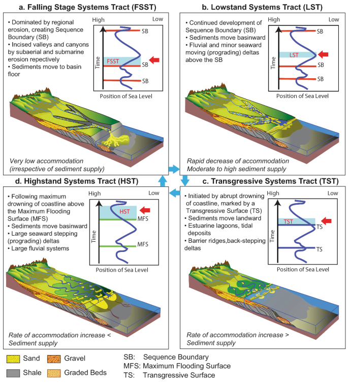

  

  Illustration after Kendall (2006) depicting predictable lateral shift of facies under varying accommodation versus supply scenarios dictated by the position of sea level. A sequence is defined as a full cycle of depositions between two sequence boundaries (generated by a Falling Stage Systems Tract—FSST—and/or Lowstand Systems Tract—LST). See Glossary of Terms for further explanations of different systems tracts and their stratigraphic markers. See Electronic Supplementary Material for a video illustrating these concepts (ESM_2)

Over the years, several professionals (Sugarman and Miller 1997; Ehman and Edwards 2014; Meyer et al. 2016; Shultz et al. 2017; Samuels and Sadeque 2021) have successfully applied the principles of sequence stratigraphy to address hydrogeological and environmental issues. However, since contaminated sites often also include continental depositional environments or tectonically-controlled settings (Fig. 4.6), the application of sequence stratigraphy is not always straightforward. Therefore, a ‘fit for purpose’ adaptation of the methodology is recommended and is discussed further in the following section.

4.4 Methodology

4.4.1 Application of Sequence Stratigraphic Principles at Contaminated Sites

One of the biggest challenges for stratigraphic correlation in the environmental industry is the lack of reliable datasets. Sediment cores are seldom intact and preserved, while field-descriptions of lithology from driller’s logs are frequently limited and sometimes biased. Moreover, many sites are shallow—typically less than 150 m below ground surface (m bgs) and, in the case of LNAPL-contaminated sites, often less than 20 m bgs—and limited in scale (several thousand square meters or less).

Considering these limitations, this section proposes a practical, iterative approach to implement sequence stratigraphic principles and facies architecture analysis at contaminated sites. This methodology is applicable to any contaminated site within shallow marine and continental depositional environments.

4.4.2 Evaluation of Geologic Setting and Accommodation

Having a thorough understanding of regional geological setting is key to evaluating site datasets in terms of allocyclic factors (Table 4.1) and making more informed correlation decisions. This regional understanding can be achieved through the study of surface and subsurface geological maps, global sea level curves (Haq and Schutter 2008), and reports on tectonic and climatic history, among others.

Within this regional context, a knowledge of site-specific local depositional environments from previous reports and academic publications helps to understand the autocyclic controls on facies architecture governing local accommodation (Table 4.1). Geological investigations of contaminated sites initiate with an in-depth research for existing reports and papers that define the structural and depositional history of the targeted subsurface interval for the site. In the United States, regional and local geological information can be found in many public sources such as the United States Geological Survey (USGS), state geological surveys, universities, research institutions, local governments, published literature—e.g., Geological Society of America (GSA), American Geophysical Union (AGU), American Association of Petroleum Geologists (AAPG), and Society for Sedimentary Geology (SEPM)—and state database websites. Also, application of modern depositional analogs using Geographic Information System (GIS) and remote sensing data, as well as outcrop investigations (nearby gravel pits, cut banks, road cuts, quarries), can be useful for estimating width/thickness ratios of relevant clay deposit/sand-body geometries (e.g., Fielding and Crane 1987; Reynolds 1999; Gibling 2006) and to provide additional insights for subsurface heterogeneity as exemplified in Fig. 4.9. This strategy is particularly helpful in instances where good spatial and/or vertical data coverage at the site is lacking.

Fig. 4.9

Panel demonstrating how ancient and modern analog data can be used to enhance geologic correlation at a site. a Shows an outcrop of a meandering river system located close to a contaminated site. The relict river had migrated from right to left until it was eventually abandoned and ‘plugged’ with fine-grained sediments. b Depicts the method of identifying bedset boundaries (black markers) and bar boundaries (blue markers) for detailed correlation of the fluvial deposits by recognizing bounding discontinuities. Note the boulder-sized (0.3–0.6 m thick) rip-up clasts within the same outcrop, which reveal that thick clay deposits captured within nearby site boring logs may represent localized features rather than laterally continuous floodplain deposits. c shows how integration of outcrop measurements with Google Earth imagery provides a basis for determining appropriate width/thickness ratios of facies beneath the site for guiding correlation lengths between boreholes (Fielding and Crane 1987). See Electronic Supplementary Material for an uninterpreted version of Fig. 4.9b) (ESM_3)

4.4.3 Analysis of Lithologic Data

Grain size and sorting are two lithologic characteristics that can significantly influence a unit’s pore space geometry and permeability. In general, coarse-grained, well-sorted units exhibit higher permeability, while finer-grained and/or poorly sorted units display lower permeabilities. Therefore, defining changes in grain size and sorting within the existing dataset is critical for defining preferential migration pathways through both the vadose and saturated zones.

Borehole logs, geophysical logs (e.g., gamma, resistivity, neutron-porosity), CPT logs, Hydraulic Profiling Tool (HPT) logs, Electric Conductivity (EC) logs, and several other site characterization tools discussed in Chap. 7 are commonly used to provide valuable information for the classification of sediments at contaminated sites. Borehole core description ideally provides the ‘ground truth’ for accurate grain size and sorting information of sedimentary deposits. Therefore, great care must be taken to acquire high-quality data. Although often underutilized in the environmental industry, the Wentworth scale (Wentworth 1922; Fig. 4.10a) of grain size measurement is preferred over the Unified Soil Classifications System (USCS) classification (Fig. 4.10b) because it provides more precise grain size measurements for understanding depositional processes from borehole data. Moreover, once a grain size distribution is measured in the Wentworth scale, it can easily be broken down into the USCS classification for engineering purposes. On the other hand, if the data is lumped under the USCS classification, it is more difficult to be converted into the Wentworth scale.

Fig. 4.10

A Comparison between the Wentworth scale and the USCS classification. Observe how grain size is combined with texture in the USCS classification. This method may be convenient for measurements by sieve. On the other hand, the Wentworth system is purely based on grain size differences measurable in the field by a hand lens and grain size comparator available in the market while giving a higher resolution of grain size variation

Grain size measured in the Wentworth scale can be hand-plotted as a grain size log that reveals accurate grain size trends of the core data (Fig. 4.11a). However, processing previously obtained data in USCS classification can be also utilized for stratigraphic work, typically by color-coding the grain size and texture data (Fig. 4.11b) that are lumped within the USCS classes.

Fig. 4.11

Processing vertical grain size and texture from borehole using Wentworth and USCS data for calibration with geophysical logs. Blue arrows show coarsening-upward and red arrows show fining-upward trends in the vertical profile. a Separates grain size data from texture information and identifying vertical grain size trends (fining-upward/coarsening-upward) in Wentworth scale in hand-drawn log. b Color-codes grain size and texture to represent data collected in USCS scale. c Illustrates the calibration of gamma logs to borehole grain size data to use as proxy for continuous grain size logs. API (American Petroleum Institute) value is the unit of natural gamma radiation of sediments

Despite the utility of borehole logs for accurate field measurements of lithology, they are limited by discrete sampling intervals and inherent logging biases. Therefore, a best-practice strategy to achieve a continuous, unbiased picture of subsurface conditions is to calibrate borehole logs with geophysical logs (e.g., gamma log, Fig. 4.11c).

Since good data quality is the first precondition for accurate and meaningful stratigraphic correlation, emphasis should be given in having multiple data types for individual boreholes (e.g., borehole core description supported by HPT, CPT, gamma, and resistivity logs).

4.4.4 Facies Architecture Analysis

Once the grain size and textural data (including sorting) have been processed, the identified grain size trends (Fig. 4.11) and lithologic compositions are compared with relevant facies models (see discussion in Sect. 4.1.2) for different depositional environments (Fig. 4.12) recognized during regional research (Fig. 4.13). Their spatial relationships are then determined using Walther’s Law.

Fig. 4.12

Illustration showing major depositional environments (abbreviated as ‘Env.’) and their sub-environments. Note that while not all depositional processes are contemporaneous, the geology of a site may be dictated by multiple depositional environments over time

Fig. 4.13

Vertical grain size profiles with sedimentary structures typical of a variety of depositional environments. Black arrow indicates direction of grain size coarsening observed in boreholes. Responses of grain size trends are also captured in GR, EC, and CPT logs. Note that different facies may exhibit similar log motifs, emphasizing the need to place them within the context of the regional geology before correlation

The hierarchy of three-dimensional architectural components (elements) of the depositional facies (e.g., shoreface, delta mouth bar, fluvial channel bars, alluvial fan sheet flood deposits, etc.) are further analyzed by recognizing the internal stacking patterns, geometry, and relationship of bounding surfaces shown by the data or its analog (Fig. 4.9). This determination of hierarchy in facies architecture ultimately helps to distinguish the larger stratigraphic architecture of sequences (i.e., hierarchy and stacking patterns of their building blocks—i.e., parasequences) resulting from allocyclicity and is critical for predicting aquifer heterogeneity across multiple scales. Figure 4.14a shows how the three-dimensional hierarchy of facies is established on the basis of an order of bounding surfaces from beds to elements. Figure 4.14b shows how stratigraphic architecture is understood in relation to stacking pattern and hierarchy of large-scale architectural units (elements and above) under allocyclic controls (e.g., sea level changes).

Fig. 4.14

a Example of facies architecture hierarchy in a coastal setting of shoreface deposits. The scale of architectural units increases from top to bottom (conceptualized after Vakaralov and Ainsworth 2013). b Conceptual cross-sections (adapted from Van Wagoner et al. 1990) showing stratigraphic architecture of coastal deposits based on large-scale stacking patterns related to sea level changes. Parasequences developed between marine flooding surfaces show aggradational, progradational, or retrogradational stacking patterns depending upon the accommodation versus sediment supply scenario of the system

A key take-away from this approach is to recognize that it can address heterogeneity across multiple scales. Because scaling is often a challenge encountered by groundwater modelers and remedial practitioners, this approach can serve as an invaluable tool for developing more effective remedial strategies.

4.4.5 Correlation Between Boreholes

The key to successful correlation is to correctly identify time-significant surfaces (time markers) before populating the facies architecture between those surfaces. Determination of the relevant accommodation scenarios based on this approach has direct bearing on understanding the aquifer heterogeneity of a site.

4.4.5.1 Marine and Coastal Environments

If the target remedial zone of a contaminated site was deposited in a marine or coastal setting, correlation of the identified facies and propagation of the facies architecture should be conducted within a conventional depositional sequence stratigraphic framework based on the accommodation scenario and recognizable systems tracts (Fig. 4.8). The defining time-significant surfaces include marine flooding surfaces (e.g., mud or shale markers), wave ravinement surfaces, and regional erosional boundaries (sequence boundaries). Standard concepts and the basic methodology of sequence stratigraphy are described in numerous articles and books (Van Wagoner et al. 1990; Emery and Meyers 1996; Posamentier and Allen 1999; Catuneanu 2006; Embrey 2009). Once several cross-sections are developed (preferably both in dip and strike directions of a depositional system) and a three-dimensional understanding of the subsurface heterogeneity is attained (Fig. 4.15), this framework should be integrated with hydrogeologic and chemical data to interpret the hydrostratigraphic units for the site.

Fig. 4.15

Fence diagram composed of sequence stratigraphic correlations from a contaminated site that lies within the New Jersey coastal plain (USA). Hydrostratigraphic units were determined by integrating site hydrologic data into this three-dimensional stratigraphic framework (Sadeque 2020)

4.4.5.2 Continental and Tectonically-Controlled Settings

For a site in which the target depth interval of aquifer is recognized to have been deposited in a fluvial, alluvial fan, aeolian (loess), glacial, or structurally-controlled setting, we recommend the application of allostratigraphic methods (‘descriptive sequence stratigraphy’ after Brookfield and Martini 1999) to correlate and address the critical issues with the application of depositional sequence stratigraphy in the continental environments (summarized in Sect. 4.3 and Table 4.1).

This correlation approach, also informally designated ‘Environmental Sequence Stratigraphy’ (ESS) within the environmental industry (Shultz et al. 2017; Samuels and Sadeque 2021), primarily relies on defining and naming mappable discontinuity-bounded depositional successions without placing particular emphasis on the type of discontinuity used as a fundamental stratigraphic break.

The following are some of the common markers of mappable discontinuity that have time-significance for correlation:

• 1. Regional flooding surfaces, e.g., created by cyclic flooding events in continental fluvial settings, clay layers resulting from major channel migration and avulsion events, sheet-flood episodes in alluvial fan settings, and flooding surfaces related to glacial outwashes and glacial catastrophic events indicated by mud/shale markers and erosional features.

• 2. Major facies dislocations indicated by abrupt ‘shallow facies’ over ‘deep facies’, e.g., glacial over non-glacial facies and vice-versa.

• 3. Significant paleosol horizons and coal/peat horizons (in continental fluvial environments), caliche horizons (in alluvial fan environments), loess horizons (fine-grained aeolian deposits), and outwash (sandur) plain boundaries (in glacial environments).

• 4. Tectonically-driven incised valley boundaries, autocyclic fluvial erosions, bypass or erosional supersurface (in aeolian environment), and various glacial incisions, etc.

Pervasive markers that can be correlated over the entire region probably represent the allocyclic controls of tectonics and/or climate. Other markers local to the specific site may reflect autocyclic processes. But even if the distinction between these two types of markers is not always conclusive due to incomplete dataset, this approach of utilizing mappable discontinuities (Figs. 4.9b and 4.16) in combination with facies architecture analysis leads to a predictable time-significant framework of correlation.

Fig. 4.16

Example of correlation by identification of bounding discontinuities in a structurally-controlled contaminated site in the Washington DC area using EC logs and conductivity (K) logs. a Correlation utilizing both major and minor bounding discontinues (time markers) in a horst and graben system. The faults were identified from regional research and ‘slicken-sides’ were identified using cores from the site. b Up-close excerpt of correlation showing the time markers in detail

4.4.6 Integration with Hydrogeology and Chemistry Data

Once the stratigraphic framework has been established, it should then be integrated with hydrogeologic and chemical data to guide the reinterpretation of site hydrostratigraphic units. Screen intervals, groundwater levels, and chemistry data (preferably color-coded by level of contamination) are just some examples of relevant data that should be added to the cross-sections to aid in the reinterpretation within the context of the stratigraphy. There must be agreement between interpreted stratigraphic pathways, potentiometric trends (vertical gradients and mapped trends), and analytical (isoconcentration) contours. The new understanding of subsurface conditions derived from this synergy should be used to redefine preferential groundwater flow paths and redraw hydrogeological contours that are more representative of the subsurface conditions of a site.

Figure 4.17 provides a generalized workflow for stratigraphic correlation as described in this chapter. Identifying depositional facies for the site data (by comparing with facies models and depositional analogs) and developing a stratigraphic framework for the depositional facies (using stratigraphic markers) are the two critical parts of the correlation process. Incorporating groundwater and chemistry data, as well as showing well screen intervals in the correlation provides a holistic view of the subsurface needed for developing an optimal remedial strategy at a site. Observe that following flow paths 1–5 lead to correlation by only facies analysis, whereas the flow paths of I–II and Ia–IIa help develop the sequence stratigraphic framework. The input of step 5 and step III together provide a facies-based sequence stratigraphic correlation. After correlation is complete, steps 7–8 are taken to address any data gaps and provide feedback for future iterations of the process.

Fig. 4.17

Flow diagram for stratigraphic correlation proposed in this chapter. Grey boxes denote critical information required for the application of sequence stratigraphy to a contaminated site. Black and grey arrows indicate simultaneous steps taken to generate a sequence stratigraphic framework and conduct facies analysis within that framework

4.5 Case Study: Using Sequence Stratigraphy to Inform Remedial Decision-Making at a Geologically Complex LNAPL-Impacted Site

This case study aims to demonstrate how sequence stratigraphy can enhance the Conceptual Site Model (CSM) of a LNAPL-impacted site by providing a more reliable understanding of subsurface conditions and heterogeneity needed for remediation.

4.5.1 Site Background

An industrial site located in the West Coast Basin of the Los Angeles County Coastal Plain in the United States (Fig. 4.18) has been an active industrial facility for almost a century. The site is geologically complex and is impacted by various petroleum products. The remedial objective for the site is to implement aerobic bioremediation via biosparging at targeted zones with impacts to prevent the off-site migration of LNAPL.

Fig. 4.18

Modified from U.S. Geological Survey. Public domain. Credit Miranda Fram

Approximate geographical location of the site (shown in blue box) in the West Coast Basin of California, USA.

Traditional studies of the subsurface geology of the region for groundwater evaluations (Poland et al. 1956; California Dept. of Water Resources 1961; Zielbauer et al. 1962) offered subsurface stratigraphic correlations by tying together deposits of similar lithologies between boreholes without considering facies heterogeneity. The resulting ‘layer-cake’ stratigraphy led to dividing the hydrostratigraphy of the Los Angeles (LA) Basin into five major aquifers (Fig. 4.19). The present site investigation focuses on the ‘Semi-perched aquifer’, which consists of sands and gravels of ‘Recent Alluvium’ and varies between 0 and 20 m thick. The Semi-perched aquifer lies above the Gaspur aquifer, which lies at approximately 29–36 m below Mean Sea Level (MSL) and is composed of fluvial sediments of the lower Recent Alluvium.

Fig. 4.19

Generalized hydrostratigraphic framework of the site area based on a lithostratigraphic approach. The blue box denotes the stratigraphic interval of interest for the present case study. Modified figure reproduced with permission from Ehman and Cramer (1997)

Prior High-Resolution Site Characterization (HRSC) studies, including CPT with Laser-Induced Fluorescence (LIF), Membrane Interface Probe (MIP) and soil and groundwater sampling and analysis, confirmed that contamination beneath the site is concentrated within the Gaspur and Semi-perched aquifers. However, understanding of preferential contaminant migration pathways based on previous correlations proved to be inadequate for precise targeting of biosparging zones for LNAPL remediation (Fig. 4.20). This is because efficient biosparging requires adequate transmissivity of aquifer units in the target treatment zones to ensure airflow critical for aerobic biodegradation by indigenous bacteria.

Fig. 4.20

Stratigraphic correlation at the site using a lithostratigraphic approach in the semi-perched aquifer interval. Observe that while the correlation provides a general understanding of sand and clay distribution beneath the site, it does not always provide the precise resolution of heterogeneity required for targeting optimal placement of biosparging tools in high-permeability intervals

4.5.2 Application of Sequence Stratigraphy

The approach detailed in Sect.  4.4 was applied to the site to update the CSM. The objective of the sequence stratigraphic analysis was to develop a high-resolution stratigraphic framework to better define subsurface heterogeneity, characterize preferential LNAPL migration pathways, and aid in the design of targeted biosparging wells.

4.5.2.1 Evaluation of Geologic Setting–Regional Geology

The regional geology of the LA Basin (primarily consisting of the Central Basin, West Coast Basin, and the Santa Ana Coastal Basin) is described in terms of four primary structural blocks that are bound by fault zones. The site region is located on the southwestern structural block, within the LA Basin bounded by the Newport-Inglewood Fault (NIF) to the east, and the Palos Verdes Fault (PVF) to the west as shown in Fig. 4.21.

Fig. 4.21

Location and tectonic setting of the Los Angeles Central and West Coast Basins and the Santa Ana Coastal Basin (Riel et al. 2018). The blue box represents the approximate site location. The solid gold lines represent major faults in the area, including the Newport-Inglewood Fault (NIF), the Whittier Fault (WF), the Palos Verdes Fault (PVF), and the Hollywood Fault (HF). The solid blue line corresponds to the Santa Ana River. The dashed red line indicates the approximate boundary between the forebay and confined areas of the groundwater system

The LA Basin was formed during a phase of accelerated subsidence and deposition that began in the late Miocene and continued without significant interruption through the early Pleistocene. The basin was filled with thick successions of unconsolidated, stratified, and laterally discontinuous continental deposits derived from the highland areas and marine sediments to form the current broad plain. The deposits within the basin were deformed by tectonic events (folding and faulting), incised by rivers, and backfilled and buried by alluvium.

Sequence stratigraphic investigations based on seismic investigations (Ponti et al. 2007; Ehman and Edwards 2014) linked sea level changes to accommodation in the LA Basin (Fig. 4.22) and developed a robust regional sequence stratigraphic framework (Fig. 4.23). Comparison of the traditional hydrostratigraphic units relative to this sequence stratigraphic framework shows that the aquifers and aquitards possess complex internal heterogeneity on a regional scale not recognized by the traditional lithostratigraphic correlation (Fig. 4.19).

Fig. 4.22

Regional sequence stratigraphic framework for the site. The sea level curve reflects fluctuation between warm and cold climates over time, and the related development of stratigraphic sequences demarcated by sequence boundaries (after Bassinot et al. 1994; figure modified after Ponti et al. 2007)

Fig. 4.23

Reproduced with permission from Pacific Section SEPM

Detailed regional sequence stratigraphic correlation based on well logs and seismic data reflecting the impact of sea level changes on sediments (modified after Ehman and Edwards (2014)). Note that the aquifer nomenclature derived by a ‘layer cake’ lithostratigraphic approach (shown in the legend) does not necessarily correspond to the sequence stratigraphic divisions encountered in the subsurface.

4.5.2.2 Evaluation of Site-Specific Geology

The geological investigation for the site includes sediments from the shallow depth intervals of the Upper Gaspur to Semi-perched aquifer (i.e., the primary focus of this case study) as shown by the blue box in Fig. 4.23. Regional investigations (e.g., Ehman and Edwards 2014; Ponti et al. 2007) showed that both the Gaspur and Semi-perched aquifers fall within the Dominguez sequence, based on the updated sequence stratigraphic nomenclature (Ehman and Edwards, 2014). As shown in Fig. 4.22, the initiation of the Dominguez sequence corresponds to a significant sea level fall less than 15 thousand years (Ka) ago. The relatively low sea level (low accommodation) indicates that the Dominquez sequence likely developed as an incised valley fill (Fig. 4.8a). Such incised valleys are typically formed by fluvial systems that extend basinward and erode into underlying strata in response to a significant relative fall in sea level (Fig. 4.24a). This hypothesis of the incised valley is supported by published literature near the study area (Fig. 4.24b) which shows the extent of the incised valley developed during the last significant sea level fall in the region, impacting the distribution of aquifers and aquitards at the case study locality.

Fig. 4.24

Reproduced with permission from Pacific Section SEPM

a Modern incised valley example from the coast of Florida showing its various geomorphological components (modified from Google Earth image). Incised valleys can be up to several tens of meters thick and range in width from a kilometer to many tens of kilometers. b Seismic facies map of Dominguez sequence (consisting of the Gaspur and the Semi-perched aquifers) modified from Ehman and Edwards (2014). The contours in the figure represent the depth profile of the incised valley in meters.

Fig. 4.25

Idealized evolution of an incised valley-fill (IVF) in response to relative sea level changes after Shanley and McCabe (1994). The figure is modified after Shanley and McCabe (1994). The brighter colors of depositional facies in this figure represent higher transmissivity compared to the darker colored depositional facies. Although no dimension is implied in the figure, studies (e.g., Wang et al. 2019) show that the thickness of IV typically ranges from 10 to 100 m, and the width of the IVF ranges from 10³ to 10⁵ m

From the above considerations, it is predicted that the aquifer and aquitard sediments of this interval will conform to the established sequence stratigraphic model of an incised valley (Fig. 4.25) after Shanley and McCabe (1994). In Fig. 4.25, the position of sea level for each phase (1–4) is shown in red segments on the corresponding sea level curves. The first phase in the evolution of an incised valley is signified by the basinward propagation of an erosional surface (sequence boundary) accompanied by largely coastal sediment bypass (FSST). The second phase (‘Time-2’) is dominated by stacking of fluvial channel deposits in a low accommodation scenario of the LST. A tide-dominated estuarine setting ensues in the third stage (‘Time-3’) with rapidly rising sea level, following a transgressive surface shown as a blue line (transgressive systems tract or TST). Finally, in the fourth phase (‘Time-4’) with the turn-around of the sea level following a maximum flooding surface or MFS (pink line), a fluvio-deltaic setting of the highstand is emplaced (highstand system tract or HST). However, since LNAPL investigation at the site is primarily targeted within the Semi-perched zone of Recent Alluvium above the Gaspur aquifer, the stratigraphic correlation at the site is focused on interpreting aquifer heterogeneity within the upper units of the Dominguez sequence.

4.5.2.3 Analysis of Site Lithologic Data

The subsurface geological data for the CSM consisted of borehole and CPT/MIP data down to approximately 27 m bgs. Pre-existing grain size data from borehole core descriptions were represented in USCS scale (Fig. 4.10b). Apart from grain size information, other important sedimentary and biologic features necessary for detailed facies interpretations (i.e., lenticular beds, mud clasts, shell fragments, plant material, etc.) were also meticulously recorded. The grain size data was color-coded to reveal vertical grain size and texture trends in the boreholes (as exemplified in Fig. 4.11b).

CPT logs (complemented with borehole core information since CPT provides information on soil behavior type, which is not necessarily the same as sediment classification in terms of grain size) were primarily used for facies analysis at individual boreholes. Where the reliability of the secondary grain size data was in question, more emphasis was given to the CPT data for shallow depths (~30 m bgs).

4.5.2.4 Revised Geologic Framework

4.5.2.4.1 Identification of Facies

A total of eight different depositional facies were identified based on borehole core data and CPT responses with respect to the regional setting. These depositional facies are described under three facies associations below. Since the wells were very closely spaced (few meters apart), the lateral continuity of each facies of the individual facies associations between the wells could be estimated from direct observations of log responses.

• (A) Fluvial Facies Association

This depositional facies association consists of fluvial point bars, splays (crevasse splay and levee) and overbank fines (Fig. 4.26).

Fig. 4.26

a Modern analog of fluvial point bars with dimensions (modified from Google Earth image). b Vertical grain size profile of a typical point bar and associated facies conceptualized after Miall (2014). c Identification of fining-upward channel bar successions in site CPT data. The CPT information was calibrated with borehole core description for interpretation

• 1. Grain size/lithology. Grain size of point bars ranges from very coarse to medium sand, with a common presence of pebble lags and mud clasts at the erosional base. The associated splay deposits are generally finer-grained, ranging from very fine sand to silt. Overbank deposits consist of clay and silt with a high proportion of carbonaceous organic matters.

• 2. Log signatures. The CPT log signature of the fluvial point bar deposits typically exhibits a fining-upward motif (Fig. 4.26c), with a sharp base of high cone resistance (Qt) values and a gradational top of low Qt values. Locally, these units may appear ‘blocky’ which may represent downstream accretion, as opposed to the fining-upward, lateral accretion of channel bars. Splay (crevasse splay and levee) deposits are represented by thin, coarsening-upward CPT signatures associated with channel bars. Splays are marked by a gradational base of low Qt values and sharp tops of high Qt values. Overbank deposits associated with the point bar deposits show significantly low Qt values in CPT logs.

• 3. Thickness, geometry, and lateral continuity of flow units. Typically, channel point bars range in thickness from 0.50 to 1.5 m. These deposits represent single story channels with a low lateral continuity (30–150 m). The point bar deposits typically represent lenticular geometries accreting perpendicular to the flow direction of the fluvial system. Splay deposits are up to 1 m thick and show longer range of lateral continuity than point bars at the site (30–250 m).

• 4. Transmissivity. Grain size of the point bars indicates moderate to high transmissivity (conductive layers). Splays and levees represent low to moderate transmissivity, while the muddy overbank deposits are likely to have very low transmissivity (confining layers).

• (B) Bay-Head Delta Facies Association

This facies association consists of bay-head delta mouth bars and prodelta deposits (Fig. 4.27). Such deposits typically occur in a bay/estuarine setting protected from the open sea by barrier spits. However, these spits typically have low preservation potentiality, and therefore, may not be present in the sediment record.

Fig. 4.27

a Modern analog of bay-head delta mouth bar (modified from Google Earth image). b Vertical grain size profile of a typical delta mouth bar and associated facies conceptualized after Bhattacharya and Walker (1991). c Identification of coarsening-upward mouth bar successions in site CPT data. The CPT information was calibrated with borehole core description for interpretation

• 1. Grain size/lithology. Grain size of mouth bar deposits predominantly ranges from fine to medium sand with various proportions of clay and silt (5–20%). Coarse sand is observed locally. Gravel deposits are absent to rare and indications of carbonate cementation from early diagenesis are common. Prodelta deposits largely consist of silty mud, with occasional presence of shell fragments.

• 2. Log signatures. The bay-head mouth bar deposits appear ‘coarsening-upward’ to ‘spiky’ (as indicated by low Qt at the base and high Qt at the top) in CPT logs with locally ‘blocky’ responses (Fig. 4.27c). The associated prodelta deposits show uniformly low Qt values.

• 3. Thickness, geometry, and lateral continuity of flow units. Individual mouth bar units vary from 0.50 to more than 1.5 m thick. Amalgamated mouth bars locally reach a thickness of 2.4–3 m. The mouth bar units generally show high lateral continuity that ranges from 182 to more than 300 m in length. The mouth bars represent a shingled geometry of depositional units that follow the dip of the flow direction of the fluvial system.

• 4. Transmissivity. Mouth bars are inferred to be moderately transmissive (conductive layers), below the range of channel point bar deposits. Prodelta deposits are considered to have very low transmissivity (confining layers).

• (C) Tidal Deposits Facies Association

This facies association consists of tidal channel bars (Fig. 4.28) and tidal mouth bars with estuarine mudflat deposits (Fig. 4.29).

Fig. 4.28

a Modern analog of tidal channel bar (modified from Google Earth image). b Vertical grain size profile of a typical tidal channel bar conceptualized after Van Wagoner et al. (1990). c Identification of fining-upward muddy tidal channel bar successions in site CPT data. The CPT information was calibrated with borehole core description for interpretation

Fig. 4.29

a Modern analog of tidal mouth bar (modified from Google Earth image). The cross-sectional profile of an ideal tidal mouth bar is modified after Mutti et al. (1985). b Vertical grain size profile of a typical tidal mouth bar and associated facies after Mutti et al. (1985). c Identification of coarsening-upward mouth bar successions in site CPT data. The CPT information was calibrated with borehole core description for interpretation

• 1. Grain size/lithology. Grain size of tidal channel bars ranges from very fine to fine sand with a high content of mud. Tidal mouth bars range from very fine muddy sand to well-sorted fine/medium sand. Common sedimentological features of both tidal channels and tidal bars are mud-draped lenticular beds and flaser beds. Shell fragments are ubiquitous and carbonate cementation can occur locally. Rip-up clasts may be observed in tidal channels. Grain size of estuarine mudflat deposits varies from clay to silty clay. Abundant shell fragments and organic materials are present. The clay shows high plasticity (‘fat clay’).

• 2. Log signatures. The CPT log signature of the tidal channel deposits typically exhibits a fining-upward motif, with a sharp base of high Qt values and a gradational top of low Qt values (Fig. 4.28c). The tidal mouth bars show a gradational coarsening-upward motif (Fig. 4.29c) with high Qt values at the top and low Qt values at the base and have a more prominent ‘spikey’ appearance. The estuarine mudflats facies show low Qt values in general.

• 3. Thickness, geometry, and lateral continuity of flow units. The tidal channel bar deposits represent dimensions similar to the fluvial point bars at the site (0.50–1.5 m long, 100–150 m wide lenticular geometry). The tidal mouth bars are generally thinner than bay-head delta mouth bars at the site, attaining a thickness of 0.30–1 m. Amalgamation of tidal mouth bars is not identified. These tidal mouth bars represent a narrow, often ‘spikey’, shingled geometry of depositional units that follow the dip of the flow direction of the fluvial system. These units are estimated to have correlation lengths ranging from < 150–300 m.

• 4. Transmissivity. Tidal channel bars and tidal mouth bars are considered to be conductive but are inferred to have lower transmissivity than fluvial point bars and bay-head delta mouth bars. This is because of flow inhibition caused by the common presence of intervening mud laminae in both. The estuarine mudflat deposits are considered to have very low transmissivity (confining layers).

Table 4.2 summarizes the main characteristics of the depositional facies identified at the site and their implications for LNAPL migration.

Table 4.2 Transmissivity and connectivity of various depositional facies at the site

4.5.2.4.2 Correlation and Interpretation of Borehole Data

Re-correlation of the previous cross-section (Fig. 4.20) for the site using sequence stratigraphic time markers reveals a complex stratigraphic architecture at the site (Fig. 4.30) controlled by sea level-driven accommodation changes (Figs. 4.22, 4.23, and 4.24b). As discussed in Sect. 4.5.2.2, the target depth interval of this case study (Semi-perched aquifer) covers only the shallow part of the Dominguez incised valley and does not include the basal fluvial channel deposits that comprise the Gaspur aquifer. The following is a brief description of the stratigraphic interpretation from bottom to top (Fig. 4.30) that establishes the sequence stratigraphic framework for the site.

Fig. 4.30

Development of stratigraphic framework for the site based on identification of flooding surfaces and erosional markers from borehole grain size logs and CPT logs. An MFS shown in pink is identified as an important stratigraphic marker signifying the progradation of HST deposits over the predominantly tidal deposits of the underlying TST

The base of the stratigraphic interval covered in the cross-section starts above a probable transgressive surface (TS, Fig. 4.8c for illustration of concept). This surface is indicated by the signature of a regionally persistent clay-marker observed in cores and well logs that can be tied to a significant rise of sea level following the deposition of Dominguez basal fluvial channel deposits (Fig. 4.22). As the rate of accommodation generated from rising sea level exceeded sediment supply, a TST developed. This resulted in the deposition of a muddy tidal/estuarine environment and caused a landward (northward) shift of facies (see Fig. 4.8c and Fig. 4.14b-3 for concept).

Figure 4.31 shows the incorporation of depositional facies described in Sect. 4.5.2.4 to the stratigraphic framework developed in Fig. 4.30. The depositional package from −20 m above mean sea level (amsl) to −6 m amsl in this scenario is predominated by the Tidal Deposits Facies Association, as well as northward retrograding (‘back-stepping’) sediments of the Bay-head Delta Facies Association, and Fluvial Facies Association. This depositional scenario conforms to the evolution of the incised valley fill as illustrated in Time-3 in Fig. 4.25. As the generation of accommodation started to slow down over time and sedimentation outpaced accommodation, the Bay-head Delta Facies Association and Fluvial Facies Association started to prograde seaward (see concept illustrated in Fig. 4.14b-2). This significant ‘turnaround’ (e.g., seaward—southward—shift of facies) commenced following a maximum flooding of the coastline, marked by a regional mud layer (e.g., MFS) as shown in Figs. 4.30 and 4.31 (pink line), and led to the development of the HST (see concept illustrated in Fig. 4.8d). The HST is depicted from −6 to 9 m amsl and shows that the Fluvial Facies Association slowly overtopped the HST Bay-Head Delta Facies Association, eventually pushing it farther seaward (outside the visual window of the example cross-section) over time. This depositional scenario conforms to the evolution of an incised valley fill illustrated in ‘Time-4’ in Fig. 4.25. The stratigraphic model for the site within the context of the regional understanding is shown in Fig. 4.32, and helps to demonstrate how the sequence stratigraphic correlation was used to reveal distinct, predictive stratigraphic packages of depositional facies through the target interval.

Fig. 4.31

Detailed stratigraphic correlation using site CPT logs and lithologic information. Groundwater level from 2018 is shown. Observe the southward progradation of deltaic and fluvial deposits above the MFS shown in pink. Deposits below the MFS largely consist of estuarine tidal deposits and back-stepping (southward-stepping) fluvio-deltaic deposits. See Electronic Supplementary Material for an uninterpreted version of Fig. 4.31) (ESM_3)

Fig. 4.32

A three-dimensional depositional model for the site derived from sequence stratigraphic correlation of site data and regional understanding. Inferred barrier spits in the model have not been identified in the dataset, likely because of poor preservation potential. The red box indicates the approximate lateral and vertical extent of the site dataset within the established stratigraphic framework. Note that the focus of this investigation was on the Semi-perched aquifer, which only covers the TST and HST deposits of the Dominguez sequence. The data does not include the LST channel bars (Gaspur aquifer) of the Dominguez incised valley

4.5.2.5 Implications for Biosparging

The sequence stratigraphic framework derived from the correlation and interpretation of borehole data was integrated with hydrologic and chemical data to characterize preferential LNAPL migration pathways and aid in the design of targeted biosparging wells.

LNAPL was detected at the site by in-situ tooling (LIF detector response) and observations in peaks of Photoionization Detector (PID) values, as well as characterization through laboratory analysis in forensic evaluation of samples. The current water table in the area lies at a depth about −0.5 m amsl to the north and about −2.5 m amsl to the south. An overlay of LNAPL plumes on the cross-section (Fig. 4.33) shows that the peak responses correlate to zones 1–3 m below the current water table. Impacts were not detected outside of the depth intervals of 2 to −12 m amsl.

Fig. 4.33

LNAPL plumes superimposed upon the cross-section shown in Fig. 4.31. See text for detailed interpretation of LNAPL occurrences with respect to stratigraphy. Also, observe the approximate 1970 groundwater level, which helps to explain the presence of LNAPL at levels significantly lower than the present-day groundwater level

The vertical distribution of LNAPL was dictated by the regional water table which declined steadily between the 1940s and the 1970s due to pumping activities in the region, followed by a near complete rebound from the 1970s to the present (Fig. 4.34). LNAPL released prior to 1970 extended down to 18–21 m below the current water table and into more permeable sands encountered at those depths. Since the rebound of the groundwater table, much of the deeper LNAPL became confined within more permeable lower sands (tidal channel bars and tidal mouth bars) interbedded with silt and clay. The mobile LNAPL not trapped beneath a low-permeability layer was redistributed vertically within the saturated portion of the soil column, following the rising water level and creating smear zones containing LNAPL of variable pore-fluid saturation in portions of the Semi-perched aquifer. Screen intervals of some monitoring and recovery wells designed for a historically deeper water table were submerged by the rising groundwater level.

Fig. 4.34

Anthropogenic influences on groundwater at the site since the 1940s. Historic regional groundwater levels in the site area were significantly deeper than current levels. This was due to groundwater pumping between the 1940s and 1970s that lowered the local water table by as much as 18–21 m below current levels

Three major zones of LNAPL (‘LNAPL Occurrences 1–3’) were observed along the cross-section (Fig. 4.33). Note that these plume shapes were derived prior to the stratigraphic work, and their geometry is largely a product of statistical interpolation (kriging) of chemical data, rather than geological constraints on fluid flow. However, the refined stratigraphic understanding shows that the plumes were located between the upper units of the TST and the lower units of the HST facies associations.

LNAPL Occurrence-1 appeared as a large, vertically elongated LNAPL plume in the section confined to southernmost seaward part of the section between 1.5 and −14 m amsl. Transmissive units in this zone of occurrence are predominated by upper TST tidal mouth bars and lower HST bay-head delta mouth bars, along with minor tidal channel bar deposits.

LNAPL Occurrence-2 showed two individual plumes largely confined within the upper TST in the landward direction to the north between −3 to −4 m amsl and −8 to −11 m amsl. Transmissive units in this zone of occurrence include tidal mouth bars and tidal channel bars.

LNAPL Occurrence-3 was represented by the landward-most part of the upper TST to the north between −5 and −11.5 m amsl. Transmissive units in this zone of occurrence are predominated by fluvial point bars and back-stepping bay-head delta mouth bars.

As evident from the sequence stratigraphic cross-section, the occurrence, connectivity, and elevations of conductive and confining layers frequently had vertical shifts exceeding 1.5 m even with locations only a few meters apart because of the seaward dipping nature of the strata. This observation was previously unrecognized in a lithostratigraphic correlation (Fig. 4.20). Level of impacts from LNAPL concentrations was also regularly as diverse. Considering this heterogeneity, over 60 biosparging wells were installed over a distance of approximately 800 m at the site location, where design of each well was developed based on the revised stratigraphic framework and then finalized based upon each individual zone’s specific geological characteristics described in Sect.  4.5.2.4 and summarized in Table 4.2. Since the conductive layers through which LNAPL would be transported at the site appear to be predominated by thin shingles of tidal mouth bars and bay-head delta mouth bars (0.5–1.5 m thick), the screening intervals for the aerobic biosparging wells were set accordingly (in 0.5–1.5 m intervals). Thus, the revised sequence stratigraphic CSM proved essential for targeting optimal well placement/depth and aiding in the design of a more effective remedial strategy.

4.6 Summary

Subsurface heterogeneity, particularly in complex geological settings, imparts significant technical challenges in remediating LNAPL contamination and achieving cleanup goals within reasonable timeframes. Therefore, implementing a correlation approach that adequately addresses subsurface heterogeneity and reduces uncertainty between sampling locations (especially where data quality and coverage may be limited) is critical for effective remedial decision-making.

In traditional LNAPL remedial investigations, correlation has typically been conducted using ‘lithostratigraphy’, which attempts to connect sedimentary units of similar lithology, often without any scientific basis, and without recognizing the heterogeneity of subsurface sediments between boreholes. The resulting ‘layer cake’ stratigraphy of the subsurface is often too simplistic and inadequate for developing effective remedial strategies.

In contrast, the sequence stratigraphic approach (with the aid of facies models) provides a more realistic subsurface correlation based on predictable distribution of sediments in different depositional environments, and is supported by outcrop observations, seismic studies, and various laboratory flume experiments.

The key factors in sequence stratigraphy are accommodation and supply of sediments. Classical sequence stratigraphy largely focuses on understanding the heterogeneity of marine and coastal environments controlled by relative sea level changes. However, since contaminated sites are not limited to locations in marine and coastal environments, the same principles of accommodation and supply can also be extended to encompass continental environments (e.g., fluvial, alluvial fan, and glacial) where tectonics and climate play a more significant role in controlling the patterns of deposition. In these settings, autocyclic geological processes often prove to be as important as allocyclic geological processes for understanding and predicting the distribution of sediments.

The three-dimensional geologic framework derived from this inclusive correlation approach can be used to delineate the spatial heterogeneity of sedimentary units across multiple scales and to provide the theoretical validity for predicting the distribution of aquifers and aquitards beyond the existing site data set. Moreover, integration of site hydrologic and chemical data within this framework can result in precise identification of preferential contamination flow pathways. Thus, a sequence-stratigraphy-based conceptual site model is recommended for guiding remedial decision-making at LNAPL-impacted sites.

4.7 Future Directions

This chapter proposed a practical workflow for applying sequence stratigraphic techniques to continental settings. However, more theoretical studies in continental environments are necessary to further streamline a workflow that can better deal with contamination in systems such as alluvial fan and glacial settings.

Although sequence stratigraphy is gradually emerging as a best practice for environmental site management, integration of sequence stratigraphy into groundwater models remains a challenge. More research is necessary to develop a coherent methodology for integrating stratigraphic information with hydrogeology and stochastic frameworks of plume investigation through a multidisciplinary approach.

We recommend optimal spatial coverage of detailed core description (preferably using the Wentworth scale for grain size) from boreholes in combination with geophysical logs (e.g., gamma, resistivity, neutron etc.) or logs from direct-push profiling methods such as CPT and HPT (or others discussed in Chap. 7) for detailed stratigraphic correlation at a site. Application of surface geological techniques, such as shallow seismic investigation, resistivity imaging, and GPR data acquisition can further enhance high-resolution sequence stratigraphy. Complementing state-of-the-art-techniques of contamination detection (as those discussed in Chap. 8) with sequence stratigraphic correlation will provide more efficient methods for LNAPL investigation in the future.

References

Ainsworth RB, Sanlung M, Duivenvoorden STC (1999) Correlation techniques, perforation strategies, and recovery factors: an integrated 3-D reservoir modeling study, Sirikit Field, Thailand. AAPG Bull 83:1535–1551
Anderton R (1985) Clastic facies models and facies analysis. Geol Soc Lon Spec Pubs 18(1):31–47
Barrell J (1917) Rhythms and the measurements of geologic time. Geol Soc of Am Bull 28:745–904
Bassinot F, Labeyrie L, Vincent E, Quidelleur X, Shackleton N, Lancelot Y (1994) The astronomical theory of climate and the age of the Brunhes-Matuyama magnetic reversal. Earth Planet Sci Lett 126:91–108
Bhattacharya J, Walker R (1991) River- and wave-dominated depositional systems of the upper cretaceous Dunvegan formation, northwestern Alberta. Can Petrol Geol Bull 39(2):165–191
Brookfield M, Martini I (1999) Facies architecture and sequence stratigraphy in glacially influenced basins: basic problems and water-level/glacier input-point controls (with an example from the quaternary of Ontario, Canada). Sed Geol 123:183–197
California Dept. of Water Resources (1961) Planned Utilization of the Ground Water Basins of the Coastal Plain of Los Angeles County, Appendix A. California Department of Water Resources Bulletin 104:191
Catuneanu O (2006) Principles of sequence stratigraphy. Elsevier, Amsterdam
CL:AIRE (2014) An illustrated handbook of LNAPL transport and fate in the subsurface. London, UK. www.claire.co.uk/LNAPL
Ehman KD, Edwards B (2014) Sequence stratigraphic framework of upper pliocene to holocene sediments of the Los Angeles Basin, California: Pacific Section. SEPM Book 112, Studies on Pacific Region Stratigraphy 47
Ehman KD, Cramer RS (1997) Application of sequence stratigraphy to evaluate groundwater resources. In Kendall DR (ed) Proceedings of the American association of water resources symposium, conjunctive use of water resources: aquifer storage and recovery, American Water Resources Association, Herndon, Virginia, TPS-97-2: 221–230
Embrey AF (2009) Practical sequence stratigraphy. Reservoir 36:1–6
Emery D, Meyers KJ (1996) Sequence stratigraphy. Blackwell, Oxford
Farr A, Houghtalen R, McWhorter D (1990) Volume estimation of light nonaqueous phase liquids in porous media. Ground Water 28(1):48–56
Fielding CR, Crane RC (1987) An application of statistical modelling to the prediction of hydrocarbon recovery factors in fluvial reservoir sequences. SEPM Spec Pub 39:321–327
Fogg GE, Zhang Y (2016) Debates—stochastic subsurface hydrology from theory to practice: a geologic perspective. Water Resour Res 52(12):9235–9245
Freeze RA (1975) A stochastic-conceptual analysis of one-dimensional groundwater flow in nonuniform homogeneous media. J Water Resour Res 11(5):725–741
Galloway W (1989) Sequence stratigraphy; sequences and systems tract development. AAPG Bull 73(2):143–154
Gibling M (2006) Width and thickness of fluvial channel bodies and valley fills in the geological record: a literature compilation and classification. J Sed Res 76(5):731–770
Haq B, Schutter S (2008) A chronology of Palezoic sea-level changes. Science 322(5898):64–88
Huntley D, Wallace J, Hawk R (1994) Nonaqueous phase hydrocarbon in a fine-grained sandstone: 2. Effect of local sediment variability on the estimation of hydrocarbon volumes. Ground Water 32(5):778–783
James NP, Dalrymple RW (2010) Facies models 4. St. John’s; Nfld: Geol Assoc of Can
Kendall C (2006) SEPMSTRAT.org. http://sepmstrata.org
LeBlanc DR, Garabedian SP, Hess KM, Gelhar LW, Quadri RD, Stollenwerk KG, Wood WW (1991) Large-scale natural gradient tracer test in sand and gravel, Cape Cod, Massachusetts: 1. Experimental design and observed tracer movement. Water Resour Res 27(5):895–910
Lenhard R, Parker J (1990) Estimation of free hydrocarbon volume from fluid levels in monitoring wells. Ground Water 28(1):57–67
Levitt JP, Degnan JR, Flanagan SM, Jurgens BC (2019) Arsenic variability and groundwater age in three water supply wells in southeast New Hampshire. Geoscience Frontiers 10(5):1669–1683. ISSN 1674-9871
Liu JP, DeMaster DJ, Nguyen TT, Saito Y, Nguyen VL, Ta TKO, Li X (2017) Stratigraphic formation of the Mekong River delta and its recent shoreline changes. Oceanography 30(3):72–83
Mariethoz G, Caers J (2015) Multiple-point geostatistics: stochastic modeling with training images. Wiley-Blackwell
Meyer J, Parker B, Arnaud E, Runkel A (2016) Combining high resolution vertical gradients and sequence stratigraphy to delineate hydrogeologic units for a contaminated sedimentary rock aquifer system. J Hydrol 534:505–523
Miall AD (1988) Architectural-element analysis: a new method of facies analysis applied to fluvial deposits. Earth Sci Rev 22(4):61–308
Miall AD (2014) Fluvial style. In: Fluvial depositional systems (14). Springer International Publishing, p 2–68
Middleton G (1973) Walther’s Law of the correlation of facies. Bull Geol Soc of Am 84(3):979–988
Mutti E, Rosell J, Allen G, Fonnesu F, Sgavetti M (1985) The Eocene Baronia tidedominated delta shelf system in the Ager Basin. In: Mila MD, Rosell J (Eds.) Excursion Guidebook: VI Eur. Ref. Mtg. I.A.S. 13. Excursion, Lerida, Spain, 579–600
North American Commission on Stratigraphic Nomenclature (1983, Rev. 2005) North American Stratigraphic Code. AAPG Bull 89(11):1547–1591
Paola C, Straub K, Mohrig D, Reinhardt L (2009) The “unreasonable effectiveness” of stratigraphic and geomorphic experiments. Earth Sci Rev 97(1–4):1–43. ISSN 0012-8252
Poland JF, Piper AM (1956) Ground-water geology of the coastal zone; Long Beach‐Santa Ana Area, California. US Geol Survey Water‐Supply Paper 1109
Ponti D, Ehman K, Edwards B, Tinsley J, Hildenbrand T, Hillhouse J, Hanson J, Randall T, McDougall K, Powell C, Wan E, Land M, Mahan S, Sarna-Wojcicki, A (2007) A 3-dimensional model of waterbearing sequences in the Dominguez Gap Region, Long Beach, California. U.S. Geol Survey Open-File Report 2007 1013:34
Posamentier HW, Walker RG (2006) Facies models revisited. Tulsa, Okla: SEPM
Posamentier HW, Allen G (1999) Siliciclastic sequence stratigraphy; concepts and applications. SEPM 7
Reynolds AD (1999) Dimensions of Paralic Sandstone Bodies: AAPG Bull 83:11–229
Riel B, Simons M, Ponti D, Agram P, Jolivet R (2018) Quantifying ground deformation in the Los Angeles and Santa Ana Coastal Basins due to groundwater withdrawal. Water Resour Res 54(5):3557–3582
Sadeque J (2020) Role of sequence stratigraphy in remediation geology for the puchack well field superfund site, NJ. AECOM report for U.S. EPA
Samuels R, Sadeque J (2021) The application of environmental sequence stratigraphy at department of defense sites-technical report for NAVFAC EXWC
Shultz M, Cramer RS, Plank C, Levine H, Ehman KD (2017) Best practices for environmental site management: a practical guide for applying environmental sequence stratigraphy to improve conceptual site models. U.S. Environmental Protection Agency, Washington, DC, EPA/600/R-17/293
Shanley KW, McCabe P (1994) Perspectives on the sequence stratigraphy of continental strata. AAPG Bull 78(4):544–568
Smith L, Schwartz F (1980) Mass transport 1. A stochastic analysis or macroscopic dispersion. Water Resour Res 16(2):303–313
Sugarman P, Miller K (1997) Correlation of Miocene sequences and hydrogeologic units New Jersey Coastal Plain. Sed Geol 108(1–4):3–18
Vail P, Todd R, Sangree J (1977) Seismic stratigraphy and global changes of sea level; Part 5, chronostratigraphic significance of seismic reflections. AAPG Mem 26:99–116
Vakarelov BK, Ainsworth RB (2013) A hierarchical approach to architectural classification in marginal-marine systems: Bridging the gap between sedimentology and sequence stratigraphy. AAPG Bull 97(7):1121–1161
Van Wagoner J, Mitchum R, Campion K, Rahmanian V (1990) Silicislastic sequence stratigraphy in well logs, cores, and outcrops: concepts for high-resolution correlation of time and facies. AAPG Methods Explor Series 7:55
Waddill DW, Parker JC (1997) Simulated recovery of light, nonaqueous phase liquid from unconfined heterogeneous aquifers. Groundwater 35(6):938–947
Walker RG, James NP (1992) Facies Models: Response to Sea Level Change 2nd Edition. St. John’s; Nfld: Geol Assoc of Can
Walther J (1894) Einleitung in die Geologie als historische Wissenschaft. Lithogenesis Der Gegenwart Jena: g. Fischer 3:535–1055
Wang R, Colombera L, Mountney NP, (2019) Quantitative analysis of the stratigraphic architecture of incised-valley fills: a global comparison of quaternary systems. Earth-Science Rev 200
Wentworth C (1922) A scale of grade and class terms for clastic sediments. J Geol 30(5):377–392
Zielbauer E, Kues H, Burnham W, Keene A (1962) Coastal basins barrier and replenishment investigation—Dominguez gap barrier project geologic investigation. Report by Los Angeles County Flood Control District
Acknowledgements
The authors wish to thank Jay Francisco for his assistance in obtaining client-permission for sharing the case study presented in this chapter. They are especially grateful to Assaf Reese, Katherine Carr, Sarah Price, and Danielle Cebra for their outstanding support in acquiring and compiling site data, which was essential for developing this chapter. Ben Campanaro provided valuable feedback and comments to improve the manuscript. Last, but not the least, the authors would like to thank Gina DiSimone and Maryanne Cleary for their support in shaping the chapter through graphic and formatting support.
Author information
Authors and Affiliations
Corresponding author
Editor information
Editors and Affiliations
4.1 Electronic supplementary material
Below is the link to the electronic supplementary material.
Supplementary file1 (MP4 10777 kb)
Supplementary file2 (WMV 4897 kb)
Rights and permissions
Open Access This chapter is licensed under the terms of the Creative Commons Attribution 4.0 International License (http://creativecommons.org/licenses/by/4.0/), which permits use, sharing, adaptation, distribution and reproduction in any medium or format, as long as you give appropriate credit to the original author(s) and the source, provide a link to the Creative Commons license and indicate if changes were made.
The images or other third party material in this chapter are included in the chapter's Creative Commons license, unless indicated otherwise in a credit line to the material. If material is not included in the chapter's Creative Commons license and your intended use is not permitted by statutory regulation or exceeds the permitted use, you will need to obtain permission directly from the copyright holder.
Copyright information
© 2024 The Author(s)
About this chapter
Cite this chapter
Sadeque, J., Samuels, R.C. (2024). The Application of Sequence Stratigraphy to the Investigation and Remediation of LNAPL-Contaminated Sites. In: García-Rincón, J., Gatsios, E., Lenhard, R.J., Atekwana, E.A., Naidu, R. (eds) Advances in the Characterisation and Remediation of Sites Contaminated with Petroleum Hydrocarbons. Environmental Contamination Remediation and Management. Springer, Cham. https://doi.org/10.1007/978-3-031-34447-3_4
Download citation
DOI: https://doi.org/10.1007/978-3-031-34447-3_4
Published:
Publisher Name: Springer, Cham
Print ISBN: 978-3-031-34446-6
Online ISBN: 978-3-031-34447-3
eBook Packages: Earth and Environmental ScienceEarth and Environmental Science (R0)