Mastering System Monitoring and Control

Abstract

The chapter aims at exploiting the methods and tools described in the preceding parts to develop a set of selected process monitoring and control schemes. In particular, it starts with the transportation system, which operates on a set of selected routes. To measure the performance of such a system, a suitable cost function is introduced, which can be monitored and controlled by the designated supervisor. The proposed approach also allows determining the availability of the transportation system, which can be used as an additional measure for performance improvements. Subsequently, a quality control system design approach is proposed. The proposed system can be either manual or automatic. Irrespective of the selected method, it is shown how to determine a set of suitable statistical measures along with the p chart. Such a quality control system is capable of making binary quality decisions about the product being controlled. Thus, to overcome this restriction, a demerit quality control system is introduced. As a result, a set of useful statistical measures is obtained along with the practical demerit control chart. The last process monitoring strategy aims at calculating and visualizing overall equipment efficiency, which is widely perceived as a key measurement tool for assessing both productivity and efficiency. Finally, the chapter is summarized with a set of training exercises, which can be considered the master level test concerning KIS.ME-oriented skills.

5.1 Defining the Performance Cost Function and Its Control

The objective of this section is to define the performance cost function for the multiple point–single transporter system described in Sect. 3.3. The process starts with providing the availability of the transportation system. Subsequently, the performance cost function is defined over a set of routs. Thus, the entire performance is related with the sum of all cost functions divided by the total run time.

Let us start defining the work environment for the transporter operator:

• Routes: The transporter operates within Workpsace 1 according to the routs presented in Fig. 5.3.

• KIS.Device: The transporter operator uses KIS.BOX Transporter to signify the start and finish of a given transportation task.

• Route assignment: The route assignment is realized by the KIS.MANAGER operator, which is setting KIS.Box Transporter Button 1 operational LED color to the one corresponding to the desired route.

> System operators

It is important to stress the fact that there are two operators within the system:

• KIS.MANAGER operator: A human being assigning a transport task within a selected route and monitoring its realization.

• Transporter operator: A human being physically realizing transportation tasks.

Let us start with implementing a single route system, i.e., a blue one, and calculating transporter availability, which is defined as

$$\begin{aligned} \text{ Availability }=\frac{\text{ Run } \text{ time }}{\text{ Planned } \text{ transportation } \text{ time }}, \end{aligned}$$

(5.1)

where the run time is the amount of time spent on the transportation whilst the planned transportation time is obtained as follows:

$$\begin{aligned} \text{ Planned } \text{ transportation } \text{ time }=\text{ Shift } \text{ length }-\text{ breaks } \end{aligned}$$

(5.2)

and signifies the time span in which the transporter can be operational. As an example, let us consider an eight-hour shift with a one-hour break, which gives

$$\begin{aligned} \text{ Planned } \text{ transportation } \text{ time }=\text{480 }-\text{60 }=420 \text{(min) }. \end{aligned}$$

(5.3)

Table 5.1 Set of possible routes

As can be observed in Table 5.1, the idle state corresponds to the time in which the transporter is not realizing any transportation. However, before proceeding to the implementation, let us define the transportation acknowledgement and realization procedure:

• 1. The KIS.MANAGER operator sets the color of the KIS.BOX Transporter Button 1 operational LED to the one corresponding to a desired route.

• 2. The transporter operator acknowledges and starts the transportation action by pressing KIS.BOX Transporter Button 2.

• 3. The KIS.BOX Transporter Button 2 operational LED changes its color to the same as the one of the KIS.BOX Transporter Button 1 operational LED.

• 4. The KIS.BOX Transporter Button 1 operational LED color is changed to black.

• 5. The transporter operator accomplishes the transportation and then presses KIS.BOX Transporter Button 2.

• 6. The KIS.BOX Transporter Button 2 operational LED color is changed to black.

Note that, after Step 4 of the above procedure, the KIS.MANAGER operator can arrange a consecutive route by setting the KIS.BOX Transporter Button 1 operational LED color. The implementation of Steps 1–4 can be realized with five rules like the sample one for the blue route, which is given in Fig. 5.1. The rules for different routes can be implemented in a similar way, and hence they are omitted. Finally, the rule implementing Steps 6–7 is given in Fig. 5.2. It is also assumed that each route has an associated ideal route time. These times should be perceived as optimal performance goals on a given route (see Table 5.2). Having these data, one can define a performance cost function over the processing period:

$$\begin{aligned} J=\frac{1}{t_r}\sum _{i=1}^{n_r}n_it_i, \end{aligned}$$

(5.4)

where $t_r$ is the run time within the processing period, $n_r=5$ is the number of routes (cf. Table 5.2), $t_i$ is the ideal transportation time of the i-th route while $n_i$ is the number of cycles on the i-th route. Thus, in the ideal case, this the above function should be equal to 1, which signifies perfect performance of the transporter.

Fig. 5.1

Sample rule for acknowledging Route 1

Fig. 5.2

Rule for accomplishing the transportation action

Table 5.2 Routes and ideal route times

Let us start with the KPI which can be used for the calculation of (5.1) with KIS.BOX Transporter. For that purpose, it is assumed that the planned transportation time is equal to 420 min (cf. 5.3):

where x is an alias name of button2ColorKpiDuration. Note that the KPI starts with determining all durations for a non-idle state, which is equivalent to the black color of the KIS.BOX Transporter Button 2 operational LED. To get a fair assessment of (5.1), the results provided by the above KPI should be aggregated within an eight-hour shift using the sum aggregation mechanism. This can be achieved with the KPI Aggregated Chart, which can group the results in a selected aggregation period, i.e., an hour or a day. An alternative approach is to calculate the availability within a given processing period, which can be realized as follows:

Finally, an average availability can be calculated and visualized using KPI charts. Let us proceed to the implementation of (5.4), which should be started with introducing $n_r=5$ ideal transportation times (cf. Table 5.2):

Fig. 5.3

Floorplan with a set of routes

The next step boils down to calculating the number of cycles on a given route $n_i$, $i=1,\ldots ,n_r$. For that purpose let us recall the numerical counterparts of colors, which are given in Table 2.2. The implementation consists in calculating the number of KIS.BOX Transporter Button 2 operational LED color changes. This can be realized using led2ColorKpi with an associated alias variable y. As a result, the KPI code can be extended as follows:

The last stage of the implementation is to calculate the run time $t_r$ and the current value of the performance function (5.4):

Let us consider a sample transportation request sequence, which is presented in Fig. 5.4. In particular, there are 15 transportation requests, which are ordered by the KIS.MANAGER operator using the KIS.BOX Transporter Button 1 operational LED color (cf. Sect. 2.6). Association of a given route with the assembly stations (A1–A3) is depicted as well. Using Table 5.2 and Fig. 5.4, one easily see that there are four cycles for route 1, three for route 2, three for route 3, three for route 4 and two for route 5. The objective of the remaining part of this section is to show evolution of the performance and availability of the implemented system, which was calculated using the KPI Aggregated Chart grouped by the hour. Moreover,

• availability within a processing period, and

• the performance cost function

were also calculated for KPIs using a 60-min processing period. The obtained results are given in Table 5.3. As can be observed, 0.25 availability in the 5th hour is caused by the scheduled 45-min break. A similar effect is also visible in the 17 h due to a 15-min break. In most cases the performance function is close to its optimal level, which is equal to 1. Note that both availability and the performance cost function can be also interpreted in percents of their maximum respective rates. This can be easily achieved by multiplying them by 100.

Fig. 5.4

Sample transportation request sequence

Table 5.3 Availability and performance cost function

5.2 Monitoring the Product Rejection Rate

The objective of this section is to show a sample implementation and analysis concerning two product rejection rate monitoring schemes. In both cases, it is assumed that the number of tested products is not constant within the processing period. Let us start with the first case, which is implemented using the following environment:

• KIS.Device: The operator controlling the quality of produced items is equipped with KIS.BOX, which is operating within Workspace 1.

• Item rejection/acceptance: If an item is acceptable, then the operator pushes KIS.BOX Button 1 while KIS.BOX Button 2 is pushed otherwise.

Let us start with implementing the KPIs for calculating

• the total number of tested items per processing period,

• the number of rejected items per processing period.

The implementation of the first KPI boils down to counting how many times both KIS.BOX buttons were pushed, which can be performed as follows:

where pass and fail are aliases of button1Pressed and button2Pressed, respectively, while total stands for the total number of tested items. The implementation of the second KPI can be performed by suitably reducing the preceding one, which yields

Table 5.4 presents the obtained results concerning 20 consecutive processing periods. Note that in all cases the processing period was equal to one hour. From these results it is evident that there are in total

$$\begin{aligned} N=\sum _{i=1}^{20}n_i=953 \end{aligned}$$

(5.5)

items, among which

$$\begin{aligned} N_r=\sum _{i=1}^{20}n_{r,i}=76 \end{aligned}$$

(5.6)

are of unacceptable quality, and hence they are rejected. Thus, the ratio between the rejected and the total number of items can be obtained as follows:

$$\begin{aligned} \bar{p}=\frac{N_r}{N}=0.0797. \end{aligned}$$

(5.7)

This means that the rejection rate is around $8\%$.

Table 5.4 Quality test results

The objective of the subsequent deliberations is to develop the p chart (cf. Sect. 4.4.2), which can be used for statistical process control pertaining to the quality of the manufactured items. Let us recall that the p chart is designed according to the following principle:

• Center line: $\bar{p}$,

• Upper control limit (UCL):

  $$\begin{aligned} \text{ UCL }=\bar{p}+3\sigma _p=\bar{p}+3\sqrt{\frac{\bar{p}(1-\bar{p})}{n}}, \end{aligned}$$

  (5.8)

• Lower control limit (LCL):

  $$\begin{aligned} \text{ LCL }=\bar{p}-3\sigma _p=\bar{p}+3\sqrt{\frac{\bar{p}(1-\bar{p})}{n}}. \end{aligned}$$

  (5.9)

The main assumption concerning the above principle is that the total number of samples is constant in each (i-th) processing period. Unfortunately, due to manual testing, such an assumption is too restrictive. Thus, one way out of this problem is to assume an average number of items per processing period. Another solution is to calculate the LCL and the UCL for each processing period separately. The KPIs calculating the UCL and the LCL for a varying n and $\bar{p}$ are as follows:

UCL:

LCL:

Note that the LCL cannot be lower than zero, and hence there is a need for using the Max[] function. Finally, the center line (CL) is simply given by (5.7), which implies the KPI below:

while the monitored rejection rate p should be calculated using the following KPI:

To illustrate the UCL and LCL calculation according to (5.8)–(5.9), let us consider a sample processing period in which $n=30$. Thus, Eqs. (5.8)–(5.9) yield $\text{ UCL }=0.228$ while $\text{ LCL }=\max (-0.069,0)=0$. Indeed, the rejection rate cannot be negative, and hence the LCL is set to zero.

Finally, using a set of four developed KPIs, one can design the p chart. Thus, according to the approach presented in Sect. 4.4.2, the above KPIs should be suitably associated with the KPI Aggregated Chart. The obtained results are presented in Fig. 5.5. For better illustration, the results are also gathered in Table 5.5. As can be observed, for the six processing periods being presented the ratio p oscillates around the center line and does not exceed the control limits.

Fig. 5.5

Chart p for manual quality control

Table 5.5 Quality test results

Fig. 5.6

KIS.LIGHT Input 1

Let us proceed to the second case, i.e., an automatic quality control system. It uses KIS.LIGHT as a communication means between an automatic quality control system and KIS.MANAGER. In particular, KIS.LIGHT Input 1 receives a false–true–false sequence when the controlled item satisfies the quality requirement. Otherwise, a false–true–false sequence is sent to KIS.LIGHT Input 2. Figure 5.6 presents a sample KIS.LIGHT Input 1 sequence forming the basis for calculating the number of items which pass the quality test. As in the manual case, let us start with implementing the KPIs for calculating

• the total number of tested items per processing period,

• the number of rejected items per processing period.

Let us proceed to the implementation of the first KPI, which can be realized using the RisingEdge command. It counts the number of false–true sequences, and hence the KPI boils down to

where pass and fail are aliases of input1Status and input2Status while, respectively, total stands for the total number of tested items. As previously, the number of items which do not satisfy the quality test can be easily obtained with the KPI as follows:

Thus, the rejection rate p can be found:

Similarly as in the manual case, after 20 processing periods, the rejection rate was calculated as $\bar{p}=0.098$. This means that the center line can be found as in the manual case, but $\bar{p}=0.098$ should be used instead. Finally, the control limits are determined using KPIs implemented with

UCL:

LCL:

Note that the presentation of the obtained results looks similar to that for the manual case, and hence it is omitted.

5.3 Demerit System Control

The objective of the previous section was to describe a quality control system which can be used for binary decisions concerning product quality, which can be either defective or non-defective. In the quality control nomenclature [1, 2], a product is perceived as a nonconforming one if it has one or more defects. In the case of complex products, several different kinds of defects may occur. It is, of course, evident that they are not equally important and serious. Thus, a suitable classification method is needed, which can handle severity of defects and weight them in a reasonable way. A demerit system [1, 2] can be a good remedy for such a situation. Traditionally, in such a system, there are four classes of defects:

Class A defect—very serious, due to which the product

• is not suitable for use;

• can fail in service and cannot be easily repaired;

• may cause a personal injury or a property damage.

Class B defect—serious, due to which the product

• will probably cause a Class A operating failure;

• will certainly cause less serious operating problems than the Class A one;

• will surely cause increased maintenance or a decreased lifetime.

Class C defect—moderately serious:

• will probably fail in service;

• may cause a problem less serious than a failure;

• will possibly have a reduced lifetime or increased maintenance costs;

• has a major defect in the finish, appearance or working quality.

Class D defect—minor, due to which the product

• will not fail in service;

• has a minor defect in the finish, appearance or working quality.

Let $n_A$, $n_b$, $n_c$ and $n_d$ represent respectively the number of Class A, B, C, D defects within the sample of n products or units. The crucial assumption is that each class of defects is independent and obeys Poison distribution [1, 2]. The expected number of defects of each class is expressed by $n\mu _a$, $n\mu _b$, $n\mu _c$ and $n\mu _d$, where $\mu _i$ denote the expected defect per unit. Thus, the number of demerits is defined as

$$\begin{aligned} d=p_an_a+p_bn_b+p_cn_c+p_dn_d, \end{aligned}$$

(5.10)

where $p_i>0$ stand for the class weight. A commonly used approach for selecting these weight is $p_a=100$, $p_b=50$, $p_c=10$ and $p_d=1$. Note that these parameters can be problem-specific, and hence they can be modified. The control limits for (5.10) can be calculated as follows [1, 2]:

Center line (CL):

$$\begin{aligned} \text{ CL }=n\left( p_a\mu _a+p_b\mu _b+p_c\mu _c+p_d\mu _d\right) , \end{aligned}$$

(5.11)

Lower control limit (LCL):

$$\begin{aligned} \text{ LCL }=CL-3\sigma _d, \end{aligned}$$

(5.12)

Upper control limit (UCL):

$$\begin{aligned} \text{ UCL }=CL+3\sigma _d, \end{aligned}$$

(5.13)

where

$$\begin{aligned} \sigma _d=\sqrt{n\left( p_a^2\mu _a+p_b^2\mu _b+p_c^2\mu _c+p_d^2\mu _d\right) }. \end{aligned}$$

(5.14)

Calculation of sample demerit control limits

Let us consider a sample demerit control system with the parameters given in Table 5.6, along with a sample of $n=200$ units. Thus, according to (5.12),

$$\begin{aligned} \text{ CL }=200\left( 100\times 0.001+50\times 0.0019+10\times 0.0194+1\times 0.01\right) =79.8, \end{aligned}$$

while (5.14) yields

$$\begin{aligned} \sigma _d=\sqrt{200\left( 100^2\times 0.001+50^2\times 0.0019+10^2\times 0.0194+1\times 0.01\right) }=57.793. \end{aligned}$$

Finally, the LCL (5.12) and the UCL (5.13) are

$$\begin{aligned} \text{ LCL }&=79.8-3\times 57.793=-93.579,\\ \text{ UCL }&=79.8+3\times 57.793=253.179. \end{aligned}$$

Note that the negative LCL should be replaced with $\text{ LCL }=0$.

Table 5.6 Demerit control system parameters

> Significance of defect per unit

The above example forms the basis for developing a chart for assuring the control of a given standard, which is shaped by $\mu _i$. This represents the expected quality level, which should take into account the economic balance between service requirements and production costs. As a result, two unappealing situations can be distinguished:

• The quality is permanently over the standard, and hence it is probable that the production is too expensive.

• The quality is permanently under the standard, and hence the cost of service/maintenance could be high. This implies the need for additional economic efforts for increasing the quality.

Under the above preliminaries, let us to proceed to the KIS.ME-based implementation. As in the previous section, it is possible to develop either a manual or an automatic demerit quality control system. However, the discussion is limited to the manual case, which employs three KIS.BOXes, i.e., KIS.BOX 1, KIS.BOX 2 and KIS.BOX 3. Once a product quality check is performed, an appropriate KIS.BOX button is pressed, which expresses the class of the product. Table 5.7 presents the association of KIS.BOXes and the defect classes. Note that most products are defect-free, and hence such a class has to be included as well. The resulting demerit system is presented in Fig. 5.7. The objective of the subsequent part of this section is to provide KPIs capable of calculating (5.10)–(5.13). However, KPIs can be implemented for a single KIS.Device exclusively. Thus, it is proposed to use appropriate rules, which will be employed to feed the information about the pressed button to a single KIS.BOX, i.e., KIS.BOX 3. Indeed, as can be observed in Table 5.7, KIS.BOX 3 Button 2 is not used, and hence it will be employed for the communication purpose. A complete set of communication rules is given in Table 5.8. Figure 5.8 presents an implementation of the first rule of Table 5.8. Having such a set of rules, it is possible to proceed to the KPI implementation. Let us start with supplementary KPIs, which can be used for calculating the number of products belonging to the classes presented in Table 5.7:

Class A:

Class B:

Class C:

Class D:

Class defect-free:

Table 5.7 KIS.BOX-based demerit quality control

Fig. 5.7

Floorplan of the KIS.BOX-based demerit system

Table 5.8 Demerit system rule base

Fig. 5.8

Sample rule of the demerit control system

where x and y are aliases of button1ColorKPI and button2ColorKPI Datapoints of KIS.BOX 3. For the implementation of (5.10)–(5.13), sample quality parameters are presented in Table 5.6. Finally, the center line and control limits of the demerit chart are given by the following KPIs:

CL:

LCL:

UCL:

The developed demerit system was validated using a one-hour processing period. First, the supplementary KPIs were employed to determine the number of products belonging to the classes defined in Table 5.7. The obtained results are presented in Table 5.9. Let us proceed to the results concerning the demerit chart, which are shaped by the monitored demerit number d. It should evolve around the center line (CL) and should be bounded by the control limits. The obtained results are presented in Table 5.10 and visualized using the KPI Aggregated Chart, which is portrayed in Fig. 5.9. The results clearly indicate that the monitored process is in the state of control.

Table 5.9 KPI-based calculation of quality control results

Table 5.10 Numerical data of the demerit chart

Fig. 5.9

Demerit chart for manual quality control

5.4 Overall Equipment Effectiveness

The main objective of this section is to show how to use KIS.ME for calculating the performance of given equipment. The discussion starts with recalling the concept of overall equipment effectiveness (OEE) [3, 4], which can be perceived as a key measurement tool for assessing both productivity and efficiency. As indicated in [4], OEE is a hierarchy of measures that exhibit how efficiently a manufacturing operation is performed. This indicator is stated in a very general form, and hence it makes it possible to perform an efficient comparison between manufacturing units in different departments, organizations, etc. The core features of OEE are as follows [3, 4]:

• identification of equipment potential;

• identification and tracking of the losses;

• identification of opportunities for increasing equipment performance.

As a result, OEE can be used for

• increasing productivity,

• decreasing the overall cost,

• increasing the awareness about equipment productivity,

• extending the equipment operational life time.

The crucial components of OEE are the following:

availability:

$$\begin{aligned} \text{ A }=\frac{t_P-t_S}{t_P}=\frac{t_R}{t_P}, \end{aligned}$$

(5.15)

where $t_P$ is a planned production time, $t_S$ stands for the unplanned stop or downtime, while $t_R$ signifies the run time.

Performance:

$$\begin{aligned} \text{ P }=\frac{t_i n_p}{t_P-t_S}=\frac{t_i n_p}{t_R}, \end{aligned}$$

(5.16)

where $t_i$ is the ideal single part manufacturing time and $n_p$ stands for the total number of manufactured parts, i.e., both defective and defect-free ones. Quality:

$$\begin{aligned} \text{ Q }=\frac{n_p-n_d}{n_p}=\frac{n_g}{n_p}, \end{aligned}$$

(5.17)

where $n_d$ and $n_g$ stand for the number of defective and defect-free parts, respectively.

Finally, the OEE indicator is simply given by

$$\begin{aligned} \text{ OEE }=\text{ A }\times \text{ P }\times \text{ Q }. \end{aligned}$$

(5.18)

The objective of the remaining part of this section is to show how to employ KIS.ME for calculating OEE. It can also be expressed in percents, which can be easily attained by multiplying (5.15)–(5.17) by 100. Note that a world class value of OEE should be at the level of 85% or higher. Let us also note that the calculation of planned production time obeys

$$\begin{aligned} t_P = t_A - t_B, \end{aligned}$$

(5.19)

where $t_A$ and $t_B$ stand for the available and planned break times.

Sample OEE calculation

Let us consider an example equipment, which is characterized by the parameters given in Table 5.11. According to (5.19), the planned production time $t_P = t_A - t_B=390 \text{[min] }$. This implies that $\text{ A }=\frac{t_P-t_S}{t_P}=\frac{350}{390}=0.897$ or 89.7%. Subsequently, the performance can be calculated with (5.16), which is equal to $\text{ P }=0.952$ or 95.2%. The quality is obtained with (5.17), which is equal to $\text{ Q }=0.99$ or 99%, equivalently. Finally, OEE can be calculated according to (5.18), which gives $\text{ OEE }=0.845$ or 84.5%.

Table 5.11 Sample production equipment parameters

Before proceeding to the OEE implementation, a KIS.ME infrastructure has to be defined. In particular, it should allow identification and measurement of

• the unplanned downtime $t_S$ and its cause,

• the total number of manufactured parts $n_p$,

• the number of defective parts $n_d$.

The employed infrastructure is portrayed in Fig. 5.10. As can be observed, the system has automatic quality control, which is connected with KIS.BOX digital inputs. The quality control system is actually the same as the one presented in Sect. 5.2, but KIS.BOX is used instead of KIS.LIGHT. Indeed, it employs KIS.BOX as a communication means between an automatic quality control system and KIS.MANAGER. In particular, KIS.BOX Input 1 receives a false–true–false sequence when the controlled item satisfies the quality requirement. Otherwise, a false–true–false sequence is sent to KIS.BOX Input 2. A sample sequence is presented in Fig. 5.6. Subsequently, note that the KIS.BOX Button 2 operational LED color is initially set to green using the KIS.BOX digital twin (cf. Sect. 2.6). This is a normal operation of the equipment.

Fig. 5.10

KIS.ME-based OEE data gathering scheme

Let us proceed to the identification of the cause of downtime. First, it is assumed that the equipment operator makes a decision about the current downtime state of the equipment, which may exhibit one of the modes given in Table 5.12. In particular, the state-space model concept (cf. Sect. 2.10) is utilized to change the color of the KIS.BOX Button 1 operational LED according to Table 5.12. This operation depends on the trigger which is related to pressing KIB.BOX Button 1. Once an appropriate color is selected, the equipment operator acknowledges the current state by pressing KIS.BOX Button 2. As a result, its operational LED color is changed into that of the KIS.BOX Button 1 operational LED. Thus, any alteration of the equipment state should be realized in the same way. Note also that one can freely modify or extend the states proposed in Table 5.12.

Table 5.12 Run and downtime states

Let us proceed to the KPI implementation. First, availability has to be calculated according to (5.15). For that purpose it is necessary to assume that the planned production time $t_P$ is given. Thus, let $t_A=420 \text{(min) }$ and $t_p=390 \text{(min) }$. As a result, the KPI calculating availability within a selected processing period is given by

where x is an alias of the button1ColorKpiDuration Datapoint. Finally, to assess the quality, the KPI calculation results should be aggregated with KPI charts using the SUM aggregation method (see, e.g., Sect. 4.3.2) and the $t_A$ aggregation period. Using a similar way of implementation, one can formulate KPIs calculating the sums of downtimes:

• Equipment breakdown: dred=Sum[If[x == 5,Duration[x],0]]/60000;

• Setup and adjustment: dblue=Sum[If[x == 0,Duration[x],0]]/60000;

• Minor breakdowns: dyellow=Sum[If[x == 7,Duration[x],0]]/60000;

as well as the occurrence number of such states:

• Equipment breakdown: nred=Sum[If[x == 5,1,0]];

• Setup and adjustment: nblue=Sum[If[x == 0,1,0]];

• Minor breakdowns: nyellow=Sum[If[x == 7,1,0]];

Let us proceed to performance calculation (5.16). The KPI calculating local performance within the j-th processing period, i.e.,

$$\begin{aligned} P_j=\frac{t_in_{p,j}}{t_{R,j}}, \end{aligned}$$

(5.20)

can be derived using (with $t_i=1 \text{[min] }$)

where x, y and z are aliases of button1ColorKpiDuration, input1Status and input2Status, respectively. Having k processing periods, one can aggregate the results of the above KPI. Unfortunately, there is no aggregation which makes it possible to determine total performance (5.16). A good remedy to such a problem is to define two separated KPIs:

• Ideal manufacturing time of the $n_p$ parts:

  

• Run time $t_R$:

  

and observe their relation using the KPI Pie Chart with the SUM aggregation method. Similar issues are encountered while calculating quality with (5.17). Indeed, local quality within the j-th processing period, i.e.,

$$\begin{aligned} Q_j=\frac{n_{g,j}}{n_{P,j}}, \end{aligned}$$

(5.21)

can be calculated with

Similarly, as the global quality (5.17) cannot be directly calculated, a good remedy is to define two separate KPIs:

• Number of defect-free parts $n_g$: ng=RisingEdge[y];

• Number of parts $n_p$:

  

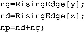
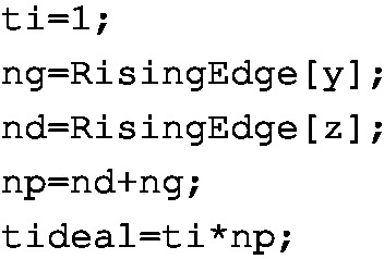
and observe their relation using the KPI Pie Chart with the SUM aggregation method. Finally, the determination of OEE can be realized directly. Indeed, by substituting (5.15)–(5.17) to (5.18), one can observe that

$$\begin{aligned} \text{ OEE }=\frac{t_in_g}{t_p}, \end{aligned}$$

(5.22)

which can be directly obtained with the following KPI:

Finally, OEE can be visualized and aggregated (with the SUM method) using a selected KPI chart.

5.5 Training Exercises

5.1

Small transportation system

Exercise requirements: The exercise requires access to one KIS.BOX.

• 1. Let us consider two transportation routes:

  • Route red:

    $$\begin{aligned} R_{r}=\left[ 1,2,3,4,5,6,7,8,9,10\right] , \end{aligned}$$

    (5.23)

  • Route green:

    $$\begin{aligned} R_{g}=\left[ A,B,C,D,E,F,G,H,I,J\right] . \end{aligned}$$

    (5.24)

• 2. Each route is going through 10 points, which can be perceived as the virtual supermarkets and assembly stations.

• 3. Each virtual transportation task is realized in the following way:

  • Step 0: set $i=1$;

  • Step 1: write the i-th name of the transportation point on a paper sheet (e.g., A);

  • Step 2: perform virtual transportation by waiting a suitable period of time;

  • Step 3: set $i=i+1$. If $i>10$, then STOP, else go to Step 1.

• 4. The ideal transportation times for the first and second route are $t_r=\frac{11}{60} (\text{ min})$ and $t_g=\frac{13}{60} (\text{ min})$.

• 5. Using the approach presented in Sect. 5.1, implement two rules for acknowledging the transportation tasks (cf. Fig. 5.1).

• 6. Implement the KPI counting the number of transportation tasks $n_r$ realized through $R_r$.

• 7. Implement the KPI counting the number of transportation tasks $n_g$ realized through $R_g$;

• 8. Implement the KPI calculating the performance of the transportation system within a processing period, which is expressed by

  $$\begin{aligned} J=\frac{1}{t_p}\left( n_rt_r+n_gt_g\right) , \end{aligned}$$

  (5.25)

  where $t_p$ is the processing period. (Hint: Use Interval[] command with transforming its value from milliseconds to minutes);

• 9. Implement the KPI calculating the availability of the transportation system within a processing period:

  $$\begin{aligned} \text{ A }=\frac{t_r}{t_p}, \end{aligned}$$

  (5.26)

  where $t_r$ stands for the run time, i.e., the duration sum for which the KIS.BOX Button 2 operational LED is not black.

• 10. Use arbitrary KPI charts to present the obtained results of (5.25) .

• 11. By using the KIS.BOX digital twin, i.e., by setting the color of the KIS.BOX Button 1 operational LED, repeat cyclically the following route assignment:

  $$\begin{aligned} R_g,R_g,R_r,R_r,R_r,R_g,R_r,R_g,R_g \end{aligned}$$

  (5.27)

  and realize each transportation task according to Step 3.

• 12. What can you say about the obtained values of (5.25) and (5.26)?

5.2

Manual quality control

Exercise requirements: The exercise requires access to one KIS.BOX.

• 1. Implement the manual quality control system presented in Sect. 5.2.

• 2. Use the Datapoint chart to visualize the system’s behaviour.

• 3. Implement the KPI calculating the number of items which pass the quality control.

• 4. Implement the KPI calculating the number of items which fail the quality control.

• 5. Implement the KPI determining the total number of tested items.

• 6. Using the KPI Pie Chart, visualize the relation between the fail/pass items.

• 7. Perform a virtual quality control action by writing consecutive natural numbers on a sheet of paper. If a number can be divided by 10, then press KIS.BOX Button 2 (fail), else press KIS.BOX Button 2 (passed).

• 8. Determine the ratio between the number of rejected and all items $\bar{p}$.

• 9. Using (5.8)–(5.9), calculate the lower and upper control limits of the p chart.

Table 5.13 Run and downtime states of the virtual production system

5.3

Virtual production system with quality control

Exercise requirements: The exercise requires access to one KIS.LIGHT.

• 1. Using Rule engine, implement a state-space model (cf. Sect. 2.10) which will cyclically change the KIS.LIGHT operational LED color according to Table 5.13.

• 2. Using the KIS.LIGHT digital twin (cf. Sect. 2.6), initialize its operational LED color to be equivalent to the run state (green color).

• 3. Using the Datapoint Chart, visualize the performance of the system.

• 4. Using Rule engine, implement a rule mechanism which during the run state (green color) will, every minute, change KIS.LIGHT digital output 1 according to the false–true–false sequence.

• 5. Using the Datapoint Chart, visualize KIS.LIGHT digital output 1.

• 6. Using Rule engine, implement a rule mechanism which during the run state (green color) will, every minute, change KIS.LIGHT digital output 1 according to the false–true–false sequence;

• 7. Using the Datapoint Chart, visualize KIS.LIGHT digital output 1.

• 8. Using Rule engine, implement a rule mechanism which during the run state (green color) will, every 45 min, change KIS.LIGHT digital output 2 according to the false–true–false sequence.

• 9. Using the Datapoint Chart, visualize KIS.LIGHT digital output 2.

• 10. let us imagine that each false–true–false sequence on KIS.LIGHT digital input 1 corresponds to a good item while the same sequence on KIS.LIGHT digital input 2 signifies a failed one. What can you say about FPY? What is the expected value of FPY?

5.4

Overall equipment efficiency of the virtual production system

Exercise requirements: The exercise requires access to one KIS.LIGHT and completion of Exc. 5.3.

• 1. Implement the p chart for the quality control system;

• 2. Select the production system available time $t_A$, and use Table 5.13 to calculate the overall planned break time $t_B$ within $t_A$.

• 3. Calculate the planned production time $t_P$.

• 4. Select a uniform processing period for all KPIs, e.g., one hour, implemented in this exercise.

• 5. Implement KPIs calculating the sum of durations corresponding to all individual states given in Table 5.13.

• 6. Visualize the KPI results obtained in the preceding point using the KPI Pie Chart with the SUM aggregation method.

• 7. Implement KPIs calculating the occurrence number of individual downtime states, i.e., equipment breakdown, setup and adjustment, minor breakdowns.

• 8. Visualize the KPI results obtained in the preceding point using the KPI Single Period Chart with the SUM aggregation method.

• 9. Implement the KPI calculating the availability of the system (5.15), and visualize the obtained results using the KPI Pie Chart with the SUM aggregation method.

• 10. Implement two KPIs calculating the number of defective $n_d$ and defect-free $n_g$ items.

• 11. Visualize the KPI results obtained in the preceding point using the KPI Pie Chart with the SUM aggregation method.

• 12. Implement the KPI calculating the total number of manufacture items $n_P$ and visualize the obtained results using KPI Aggregated Chart with the SUM aggregation method.

• 13. Analyse the results obtained in the preceding step and determine an ideal (almost impossible to achieve) manufacturing time of a single time $t_i$.

• 14. Implement two KPIs calculating an ideal manufacturing time of $n_P$ items and the actual run time $t_R$.

• 15. Visualize the KPI results obtained in the preceding point using the KPI Pie Chart with the SUM aggregation method.

• 16. Implement the KPI calculating the overall equipment efficiency (5.18) and visualize the obtained results using the KPI Single Period Chart.

5.6 Concluding Remarks

The main objective of this chapter was to utilize the methods and tools described in the preceding parts for designing a practical set of process monitoring and control schemes. All of them are relatively easy to implement and enable intuitive control of the monitored system. The chapter opened with a transportation system that operates on a set of routes. First, it was shown how to communicate the desired transportation actions between KIS.MANAGER and transporter operators. The second objective was to develop suitable measures for assessing the performance of the transportation system. For that purpose, the concept of an ideal rout time was introduced, which forms the basis for the performance cost function. Thus, with appropriate control of the transportation system, one can optimize this function. Additionally, the proposed function is very easy to interpret as its value for the optimal control is equal to 1, which can be perceived as 100% performance. The proposed approach also allows determining the availability of the transportation system, which can be used as an additional measure for performance improvements. The second process which was introduced in this chapter pertains to a quality control system, which can be either manual or automatic. Irrespective of the selected method, it was shown how to determine a set of suitable statistical measures along with the p chart. Such a quality control system is capable of making binary quality decisions about the product being controlled. Thus, to overcome this restriction, a demerit quality control system was introduced. It allows indicating various defect classes, and hence, instead of controlling the rejecting rate, it is proposed to monitor the so-called demerit number. For that purpose, the demerit chart was developed, which provides effective measures for controlling the quality of manufactured products. The last process monitoring strategy aimed at calculating and visualizing overall equipment efficiency, which is widely perceived as a key measurement tool for assessing both productivity and efficiency. In particular, it was shown how to efficiently observe availability, performance, and quality of a given manufacturing equipment. Finally, the chapter was summarized with a set of training exercises, which can be considered the master level test concerning KIS.ME-oriented skills.

References

L.A. Jones, W.H. Woodall, M.D. Conerly, Exact properties of demerit control charts. J. Qual. Tech. 31(2), 207–216 (1999)
D.C. Montgomery, Introduction to Statistical Quality Control (Wiley, London, 2020)
R.C. Hansen, Overall Equipment Effectiveness: A Powerful Production/Maintenance Tool for Increased Profits (Industrial Press Inc., New York, 2001)
D.H. Stamatis, The OEE Primer: Understanding Overall Equipment Effectiveness, Reliability, and Maintainability (CRC Press, Boca Raton, 2017)
Author information
Authors and Affiliations
Corresponding author
Rights and permissions
Open Access This chapter is licensed under the terms of the Creative Commons Attribution 4.0 International License (http://creativecommons.org/licenses/by/4.0/), which permits use, sharing, adaptation, distribution and reproduction in any medium or format, as long as you give appropriate credit to the original author(s) and the source, provide a link to the Creative Commons license and indicate if changes were made.
The images or other third party material in this chapter are included in the chapter's Creative Commons license, unless indicated otherwise in a credit line to the material. If material is not included in the chapter's Creative Commons license and your intended use is not permitted by statutory regulation or exceeds the permitted use, you will need to obtain permission directly from the copyright holder.
Copyright information
© 2023 The Author(s)
About this chapter
Cite this chapter
Witczak, M., Seybold, L., Bulach, E., Maucher, N. (2023). Mastering System Monitoring and Control. In: Modern IoT Onboarding Platforms for Advanced Applications. Studies in Systems, Decision and Control, vol 476. Springer, Cham. https://doi.org/10.1007/978-3-031-33623-2_5
Download citation
DOI: https://doi.org/10.1007/978-3-031-33623-2_5
Published:
Publisher Name: Springer, Cham
Print ISBN: 978-3-031-33622-5
Online ISBN: 978-3-031-33623-2
eBook Packages: Intelligent Technologies and RoboticsIntelligent Technologies and Robotics (R0)