Decomposition Methods

Abstract

The chapter first recalls few properties of recursive algorithms. Next, it introduces a general recursive constructive method. Finally, it presents the large neighborhood search and the POPMUSIC metaheuristics.

In the process of developing a new algorithm, this chapter should logically have been placed just after the one devoted to problem modeling. But, decomposition methods are only used when the data size to process is large. Thus, the phase is optional. The reader can glance it over before moving on to the following parts, devoted to the stochastic and learning methods. This is the reason justifying its place at the end of the first part of this book, devoted to the essential ingredients of metaheuristics.

1 Consideration on the Problem Size

The algorithmic complexity, very briefly exposed in Sect. 1.2.1, aims to evaluate the computational resources necessary for running an algorithm according to the data size it has to treat. We cannot classify the problems—large or small—only by their absolute size: sorting an array of 1000 elements is considerably easier than finding the optimal tour of a TSP instance with 100 cities. The time available to obtain a solution is clearly important: the perception of what a large instance is might not be the same if we have to perform a real-time processing in a few microseconds or a long-term planning for which a 1-day computation is perfectly convenient. Very roughly, we can put NP-hard problem instances in the following categories:

Toy Instances:

Approximative size: n ≈ 10. To ensure an algorithm works correctly, it is performed by hand. Another possibility is to compare its results to those of a method, easy to implement, but much less efficient. For instance, this can be an exhaustive enumeration of all solutions. Yet, we can empirically consider a computer is able to perform 10⁹ elementary operations per second. If one has a time budget of this order of magnitude, one can consider an exhaustive enumeration for a permutation problem instance up to n ≈ 10; for a binary variable problem, we have n ≈ 20. Naturally, for polynomial algorithms, the instance size processed in one second varies from n ≈ 50 for complexity in O(n ³) to n ≈ 10⁸ for linear complexity, passing through n ≈ 10⁴ for quadratic complexity, and n ≈ 10⁶ for an algorithm in $O(n \log \ n)$.

Small Instances:

Typical size: $10 \lessapprox n \lessapprox 10^2$. When the size no longer allows an exhaustive enumeration of all solutions, we go into the category of small instances. We could characterize them by those for which we know robust algorithms that allow getting an optimal solution in a reasonable time. It should be mentioned that the literature frequently reports exact algorithms for solving examples of “difficult” problems of much larger size than those mentioned above. However, one should be careful with such statements: indeed, optimal solutions of traveling salesman or knapsack instances with tens of thousands of elements have been found, but much smaller instances are out of the scope of these programs. Small instances are useful for designing and calibrating heuristic methods. Knowing the optimal solutions allows determining the quality of heuristics and tuning the value of their parameters while maintaining reasonable computational times.

Standard Instances:

Typical size: $10^2 \lessapprox n \lessapprox 10^4$. This is the typical application area of metaheuristics. These are frequently encountered in real-world applications. They are too large to be solved efficiently by exact methods or for a human to guess a good quality solution. The maximum instance size a metaheuristic can handle is related to its algorithmic complexity, whether in terms of computational time or memory. With more than 10⁴ elements, it becomes challenging to use a constructive method or a neighborhood size in O(n ²). This is specially the case if one has to memorize an n × n matrix for efficiency reasons. The algorithmic complexity of a metaheuristic-based program is frequently larger than O(n ³). Thus, many authors speak of a “large” instance for a size of 100.

Large Instances:

Typical size: $10^3 \lessapprox n \lessapprox 10^8$. Some real instances often have a higher number of items than standard instances, or they must be solved with less computational effort than a direct method would take. We can think, for instance, to vehicle routing for mail delivery or item labeling on a geographic map. For such problems, a size of 10⁵ is not exceptional. In this case, decomposition methods must be used. This chapter presents some general techniques for approaching large instances. Let us mention that these techniques sometimes can advantageously be applied to smaller instances, even with just a few dozen elements.

Huge Instances:

Size: n > 10⁸ items. When the size of the problem exceeds 10⁸ to 10¹⁰ items, it is no longer possible to completely store the data in RAM. In this case, it is necessary to work on parts of the instance, usually using parallel algorithms to maintain adequate processing times. The treatment of this type of instances essentially raises mainly technical issues and is beyond the scope of this book.

2 Recursive Algorithms

When a large instance has to be solved with limited computational effort, it is cut into small parts, independently solved. Finally, they are put together to reconstruct a solution to the complete problem. An efficiency gain is only possible with such a technique by the conjunction of several conditions: directly solving the problem requires a computational effort more than linear; otherwise, a decomposition only makes sense for a parallel computation. The parts must be independent of each other. Combining the parts together should be less complex than directly solving the problem. The difficulty lies in how to define the parts: they must represent a logical portion of the problem so that their assembly, once solved, is simple.

The merge sort is a typical decomposition algorithm. A list to sort is split into two roughly equal parts. These are sorted by two recursive calls, if they contain more than one element. Finally, two locally sorted sub-lists are scanned to reconstruct a complete sorted list.

2.1 Master Theorem for Divide-and-Conquer

In many cases, the complexity of a recursive algorithm can be assessed by the divide-and-conquer master theorem. Suppose the time to address a problem of size n is given by T(n). The algorithm proceeds by splitting the data into b parts of approximately identical size, n∕b. Among them, a are recursively solved. Next, these parts are combined to reconstruct a solution to the initial problem, which requires a time given by f(n). To assess the complexity of such an algorithm, we must solve the functional equation T(n) = a ⋅ T(n∕b) + f(n) whose solution depends on the reconstruction effort.

Introducing 𝜖, a positive constant forcing the function f(n) to be either smaller or larger than $n^{\log _b(a)}$, the master theorem allows deducing the complexity class of T(n) in some case:

• If $f(n) = O(n^{\log _b(a)-\epsilon })$, then $T(n) = \varTheta (n^{\log _b(a)})$.

• If $f(n) = \varTheta (n^{\log _b(a)})$, then $T(n) = \varTheta (n^{\log _b a}\cdot \log n)$.

• If $f(n) = \varOmega (n^{\log _b(a)+\epsilon })$ and if a ⋅ f(n∕b) < c ⋅ f(n), with c < 1, constant, then T(n) = Θ(f(n)).

Often, a = b: we have a recursive call for all parts. In this case, the theorem states that, if the reconstruction can be done in a sublinear time, then we can deal with the problem in linear time. If the reconstruction takes a linear time—which is typically the case for sorting algorithms—then the problem can be solved in $O(n \log n)$. The last case simply indicates all the difficulty of the algorithm is concentrated in the reconstruction operations. Finally, let us mention that the theorem does not cover all cases for the function f(n).

There are also cases where a ≠ b. An example is a query for a point of the Euclidean plane from a set of n points stored in a balanced 2D-tree (see the data structure discussed in Sect. 5.5.3.2). With such a data structure, one can halve the number of points remaining to be examined by processing a maximum of a = 2 parts among b = 4. Indeed, unlike a binary tree in one dimension, we cannot ensure to divide this number by two at every single level of the tree but only every two levels. Since this is a query problem, there are no reconstruction and f(n) = O(1). As $\log _4(2) = 1/2$, we can choose 𝜖 = 1∕2, and we are in the first case. We can deduce that the complexity of a query in a 2D-tree is in Θ(n ^1∕2). However, if the points are well spread, the empirical behaviour is better, closer to $\log n$.

Heuristic algorithms proceeding by recursion commonly stop prematurely, before the part size is so small that its resolution becomes trivial. Even if the parts are exactly solved, the reconstitution phase does not generally guarantee optimality. Hence, both cutting and reconstitution procedures are heuristics. This means that the “border areas” between two parts are, more or less obviously, not optimum. To limit this effect of sub-optimality, it is necessary to assemble as few parts as possible, while being able to process them. Indeed, if they are excessively large, their exact resolution requires too much time, or the heuristics may produce low-quality parts.

3 Low Complexity Constructive Methods

Solving large instances implies limiting the complexity of the constructive method for generating an initial solution. This means that even the most basic greedy method is not appropriate. If the function c(s, e) that provides the cost of the addition of an element e actually depends on the partial solution s, then its complexity is in Ω(n ²). Indeed, before including one of the n elements, it is necessary to evaluate c(s, e) for all the remaining elements. A random construction in linear time is not suitable, due to the bad quality of the solution produced.

It is therefore necessary to “cheat,” making the hypothesis that not all the elements of the problems have a direct relationship with all the others. Put differently, an element is in relation with a relatively limited number of other elements, and this relationship possesses a certain symmetry. It is reasonable to make the hypothesis that it is possible to quantify the proximity between two elements. In such a case, we can avoid complexity in O(n ²) by sampling and recursion. We can limit the phenomenon of sub-optimality due to the assembly of parts by stopping the recursion at the first or the second level.

3.1 Proximity Graph Construction

There are relatively good automatic classification heuristics to partition a problem of size n into k groups. The fast variant of Algorithm 2.7 (k-medoids) mentioned in Sect. 2.7.2 achieves such a heuristic partition with complexity of $\overline {O}(k\cdot n + (\frac {n}{k})^2)$.¹

This complexity can be minimized by choosing $k = \sqrt {n}$. Thus, it is possible to partition a problem of size n in $\sqrt {n}$ parts, each comprising approximately $\sqrt {n}$ elements. Performing the clustering on a random sample of the elements (e.g., $\varTheta (\sqrt {n})$) can significantly speed up the procedure. This method is illustrated in Fig. 6.1.

Fig. 6.1

Illustration of the method for partitioning a problem instance: from a complete set of n elements of the instance (a), a random sample is selected (b). Algorithm 2.7 is run on the sample and $k = \varTheta (\sqrt {n})$ medoids are identified (c). All the n elements are allocated to the closest medoid (d)

It is possible to get a decomposition with smaller clusters by applying a second recursion level: the instance is first cut into a large parts of relatively similar size as presented above. A proximity relationship is defined between large part, so that each includes O(1) neighbors. A rudimentary proximity definition is as follows: if an element has c _i as its nearest center and c _j as its second nearest, then c _i and c _j are considered as neighbors. Each large part is then partitioned into b small clusters.

Similarly, a proximity relationship is defined between small clusters. A small cluster is related to all those belonging to the large part of which it belongs. By choosing $a = \varTheta (\sqrt {n})$ and $b = \varTheta (\sqrt {n})$, we get a decomposition into a number of small clusters proportional to n, whose size is approximately identical. The overall algorithmic complexity is $\overline {O}(n^{3/2})$.

For some problems, it can make sense. Indeed, for the vehicle routing problem, the maximum number of customers that can be placed on a tour depends on the application (home service, parcel distribution, rubbish collection) and not on the total number of customers of the instance.

This decomposition technique is illustrated in Fig. 6.2. Bold lines show proximity relations between large parts. The small clusters obtained by decomposition of large parts contain about 15 elements. The elements of large parts are represented by points of the same color. By exploiting such a decomposition and proximity relationships, it becomes possible to efficiently generate a solution to a large problem instance. A computational time of about one second was enough to obtain the structures of Fig. 6.2, with more than 16,000 entities.

Fig. 6.2

Two-level decomposition of a problem instance. The elements are clustered into $\varTheta (\sqrt {n})$ large parts of approximately identical size. Bold lines show the proximity relationship between large parts. The latter are themselves decomposed into $\varTheta (\sqrt {n})$ small clusters. The complexity of the process is in $\overline {O}(n^{3/2})$. It can be applied to non-geometrical problems

3.2 Linearithmic Heuristic for the TSP

It is possible to extend this decomposition principle to a number of levels depending on the instance size and thus get an $O(n \log n)$ algorithm. This section illustrates the principle on the Traveling Salesman Problem. Rather than reasoning on the construction of a tour, we build paths passing through all the cities of a given subset.

It is actually straightforward to adapt Code 12.3 so that it is able to treat a path rather than a tour. An algorithm to optimize a path can equally be used to provide a tour. Indeed, a TSP tour can be seen as a path starting by city c _i ∈ C and ending by c _i. If we have a problem with n cities, the path P = (b = c _i, c ₁, …, c _i−1, c _i+1, …, c _n, c _i = e) defines a feasible (random) tour. The path P is either directly optimized if it does not contain too many cities, or decomposed into r sub-paths, where r is a parameter that does not depend on the problem size. To fix the ideas, the value of r is typically between 10 and 20. If n ≤ r ², a very good path passing through all the cities of P, starting in c _i and ending in c _i can be found, for example, with an ejection chain or even an exact method. This feasible tour is returned by the heuristic.

Else, if n > r ², the path P is reordered by considering r sub-paths. This is performed by choosing a sample S of r cities by including:

• u ∈ C ∖{b, e}, the city closest to b

• v ∈ C ∖{b, e, u}, the city closest to e

• r − 2 other cities of C ∖{b, e, u, v} randomly picked

A good path P _S through all the cities of sample S, starting at city b and ending at city e, can be found with a local search or an exact method. Let us rename the cities of S so that P _S = b, s ₁, s ₂, …, s _r−1, s _r, e. Path P _S can be completed to contain all the cities of C by inserting them, one after the others, just after the closest city of S. So, the completed path P _S = (b, s ₁, …, s ₂, …, , s _t, …, e) improves the initial path P. The left side of Fig. 6.3 illustrates this construction using a sample of r = 5 cities. The shaded areas highlights the first r sub-paths found.

Fig. 6.3

Recursive TSP tour construction. Left: path on a random sample (bold and light line) and reordered path P _S completed with all cities before recursive calls of the procedure. Paths P ₁ to P ₅ are drawn with different colors and different backgrounds highlight them. Right: the path P ₁ was recursively decomposed into r = 5 pieces. Final state with all sub-paths optimized

At this step, the order of the cities in the completed path P _S between two cities s _j and s _j + 1 is arbitrary (as it was for P at the beginning of the procedure). The sub-paths $P_1 = (b = s^{\prime }_1, \dots , s_2), P_2 = (s^{\prime }_2, \dots , s_3), \dots , P_r = (s^{\prime }_r, \dots , e = s_{r+1}) \subset P_S$ can be further improved with r recursive calls of the same procedure, where $s^{\prime }_j$ is the city just preceding the first one of the path P _j. The right side of Fig. 6.3 illustrates the solution returned by this recursive procedure.

It can be noted in this figure that only the sub-path P ₁ has been decomposed. The others, not comprising more than r ² cities, were directly optimized by a procedure similar to that given by Code 12.3. The solution finally obtained is not excellent, but it was obtained very quickly and is suitable as an initial solution for partial improvement techniques, like POPMUSIC, which will be detailed in Sect. 6.4.2.

4 Local Search for Large Instances

After reviewing some techniques for constructing solutions for large instances, let’s now take a look at some techniques for improving them. LNS, POPMUSIC, and Corridor assume that an initial solution to the problem is available. These techniques are sometimes called fix-and-optimize [4] or, more recently, magnifying glass heuristics [3] . The key idea is to fix a relatively large portion of the problem variables and to solve a sub-problem with additional constraints on the remaining variables. When a heuristic includes an exact optimization method, we now speak of matheuristic .

4.1 Large Neighborhood Search

Large neighborhood search (LNS) has been proposed by Shaw [5]. The general idea is to gradually improve a solution by alternating destruction and repair phases. To illustrate this principle, let’s consider the example of integer linear programming. The destruction phase involves selecting a subset of variables while incorporating some randomness into the process. In its simplest form, this consists in selecting a constant number of variables, in a completely random fashion. A more elaborate form is to randomly select a seed variable and a number of others, which are most related to the seed variable. The repair phase consists in trying to improve the solution by solving a sub-problem on the variables that have been selected. The value of the other variables being set to the one taken in the starting solution.

The name of this technique comes from the fact that a very large number of possibilities exist to reconstruct a solution. This number exponentially increases with the size of the sub-problem, meaning that they could not reasonably be extensively enumerated. Thus, the reconstruction phase consists in choosing a solution among a large number of possibilities. As the significant part of the variables preserves their value from one solution to the next, it is conceptually a local search but with a large neighborhood size. The framework of LNS is provided by Algorithm 6.1.

Algorithm 6.1: LNS framework. The destroy, repair, and acceptance functions must be specified by the programmer, as well as the stopping criterion

This frame leaves considerable freedom for the programmer to select various options:

Destroy method d(⋅):

This method is supposed to destroy part of the current solution. The authors recommend that it is not deterministic, so that two successive calls destroy various portions. Another vision of this method is to fix a certain number of variables of the problem and release the others, which can be modified. This method additionally includes a parameter that allows modulating the amount of destruction. Indeed, if the number of independent variables is too small, the repair method has too many constraints to be able to differently reconstruct the solution, and the algorithm is not able to improve the current solution. Conversely, if the number of independent variables is too large, the repair method may encounter difficulties in improving the current solution. This is peculiarly true if an exact method is used, implying a prohibitive computational time.

Repair method r(⋅):

This method is supposed to repair the part of a solution that was destroyed. Another vision of this method is to re-optimize the portion of the problem corresponding to the variables that were freed by the destroy method. One possible option for the repair method is to use an exact method, for instance, constraint programming. Another option is to use a heuristic method, either a simple one, like a greedy algorithm, or a more advanced one, such as taboo search, variable neighborhood search, etc.

Acceptance criteria a(⋅,  ⋅):

The simplest acceptance criterion is to use the fitness function value of both solutions provided as parameters:

$$\displaystyle \begin{aligned} a(s, s') = \left\{ \begin{array}{rl} True & \text{If } s' \text{ better than}~s\\ False & \text{Otherwise } \\ \end{array} \right.\end{aligned}$$

Other criteria have been proposed, for instance, those inspired by simulated annealing (see Sect. 7.1).

Stopping criterion:

The framework does not provide any suggestion for the stopping criterion. Authors frequently use the limit of their patience, expressed in seconds. Also, it can be the patience of other authors who have proposed a concurrent method! This kind of stopping criteria is hardly convincing. This point is discussed further in Sect. 11.3.4.2. The quite close POPMUSIC framework, presented in Sect. 6.4.2, incorporates a natural stopping criterion.

To illustrate a practical implementation of this method, let us consider those of Shaw [5], originally adapted to the vehicle routing problem. The destroy method selects a seed client at random. The remaining customers are sorted using a function measuring the relationship with the seed customer. This function is inversely proportional to the distance between customers and depends on whether the customers are part of the same tour. The idea is to select a subset of customers who are close to the seed one but from different routes. These clients are randomly selected, with a bias to favor those most closely related to the seed client.

The repair method is based on integer linear programming. The method implements a branch and bound technique with constraint propagation. This method can only modify the variables associated with the clients chosen by the destruction method. In addition, to prevent the explosion of computational times, common with exact methods, the enumeration tree is partially examined and heuristically pruned. A destroy-repair cycle is illustrated in Fig. 6.4.

Fig. 6.4

Illustration of LNS on a VRP instance. The initial solution (a) is destroyed by removing a few customers (b). The destroyed solution is repaired by optimally inserting the removed customers (c)

There are algorithms based on the LNS framework that have been proposed well before it. Among these applications is the shifting bottleneck heuristic for the jobshop scheduling problem [1]. In this article, the destroy method selects the bottleneck machine and frees the variables associated with the operations processed by this machine. The repair method reorders these operations, considering that the sequences on other machines are not modified. Hence, each operation on the bottleneck machine has a release time corresponding to the earliest finishing time of the preceding operation on the same job. In addition, each operation has a due date, corresponding to the latest starting time of the following operation on the same job. In this heuristic, all choices are deterministic and all optimization are exact. So, the current solution is modified only if it is strictly improved and the method has a natural stopping criterion.

The POPMUSIC method presented in the following section was developed independently from LNS. It can be seen as a less flexible LNS method, in the sense that it better suggests to the programmer the choice of options, particularly the stopping criterion.

4.2 POPMUSIC

The primary idea of POPMUSIC is to locally optimize a part of an existing solution. These improvements are repeated until no part that can be optimized are detected. It is, therefore, a local search method. Originally, this method received the less attractive acronym of LOPT (for local optimizations) [8, 9].

For large problem instances, one can consider that a solution is composed of a number of parts, which are themselves composed of a number of items. Taking the example of clustering, each cluster can be a part. In addition, it is assumed that one can define a proximity measure between the parts and that the latter are somewhat independent of each other in the solution. In the case of clustering, there are closely related clusters, containing items that are not well separated, and independent clusters, that are clearly well separated. If these hypotheses are satisfied, we have the special conditions necessary to develop an algorithm based on the POPMUSIC framework. The name was proposed by S. Voß. It is the acronym of Partial OPtimization Metaheuristic Under Special Intensification Condition.

First, let us assume that a solution s can be represented by a set of q parts s ₁, …, s _q, and next that we have a method for measuring the proximity between two parts. The germinal idea of POPMUSIC is to select a seed part s _g and a number r < q of the parts the nearest to s _g to build a sub-problem R. With an appropriate definition of the parts, improving the sub-problem, R can reveal an improvement for the complete solution. Figures 6.5 and 6.6 illustrate what a part and a sub-problem can be for various applications.

Fig. 6.5

To apply the POPMUSIC framework to a clustering problem, one can define a part as all the items assigned to the same center. The parts the nearest from the seed cluster constitute a sub-problem that is tentatively optimized independently. The optimization of well separated clusters cannot improve the solution. Hence, these parts are de facto independent

Fig. 6.6

For the VRP, the definition of a part in POPMUSIC can be a tour. Here, the proximity between tours is the distance of their center of gravity. A sub-problem consists of customers belonging to six tours

To prevent optimizing the same sub-problem several times, a set U stores the seed parts that can define a sub-problem potentially not optimal. If the tentative optimization of a sub-problem does not lead to an improvement, then the seed part used to define it is removed from U. Once U is empty, the process stops. If a sub-problem R has been successfully improved, a number of parts have been modified. New improvements become possible in their neighborhood. In this case, all parts of U that no longer exist in the improved solution are removed before incorporating all parts of R. Algorithm 6.2 formalizes the POPMUSIC method.

Algorithm 6.2: POPMUSIC framework

To transcribe this framework into a code for a given problem, there are several options:

Obtaining the initial solution:

POPMUSIC requires a solution before starting. The technique presented in Sect. 6.3 suggests how to get an appropriate initial solution with limited computational effort. However, POPMUSIC may also work for a limited instance size. In this case, an algorithm with a higher complexity can generate a starting solution.

Definition of a part:

The definition of a part is not unique for a given problem. In the VRP case, we can consider that all customers on the same tour form a part, as was done in [2, 7] (see Fig. 6.6). For the same problem, it is equally possible to define a part as a single client, as in [5].

Definition of the distance between parts:

For some problems, the definition of distance between two parts can be relatively easy and logical. For example, [9] uses the Euclidean distance between centroids for a clustering problem. For map labeling (Sect. 3.3.3), a graph is built whose vertices represent the objects to be labeled and the edges represent potentially incompatible label positions. The distance is measured by the minimum number of edges of a path to the seed label, as shown in Fig. 6.7.

Fig. 6.7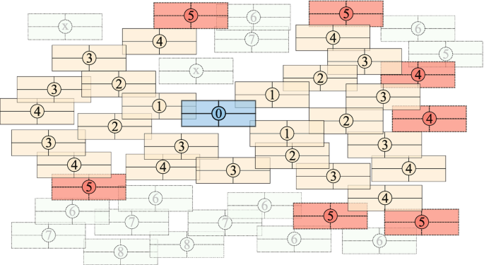

For map labeling, a part can be an object to be labeled (circle with a number). Here, we consider four possible label positions (rectangles around each object). Two objects are at a distance of one if their labels may overlap. The number inside each disc represents the distance from the seed object, noted 0. A sub-problem has up to r = 25 objects which are the closest to the seed object. Here, the distance is at most 4. The objects whose labels could collide with these r objects are included in the sub-problem. Only the positions of the labels of the r objects can be changed when optimizing a sub-problem

By cons, this definition can be quite unclear for some problems. For the VRP with time window, two geometrically close clients can have incompatible opening time windows. Therefore, they should be considered as distant.

It is possible to use several different proximity definitions simultaneously. If we take the problem of school timetable design, one definition may aim to create sub-problems focusing on groups of students following the same curriculum, another on teachers, and a third on room allocation. Of course, if several definitions of proximity between parts are used simultaneously, the last line of Algorithm 6.2 has to be adapted: a seed part s _g will only be removed from U if none of the sub-problems that can be created with s _g can improve the solution.

Selection of the seed part:

To our knowledge, there are no comprehensive studies on the impact of the seed part selection process. In the literature, only very simple methods are used to manage the set U: either stack or random selection.

Parameter r :

The size of the sub-problems depends on r, the only explicit parameter of POPMUSIC. It depends on the ability of the optimization method. A low value only allows minor improvements, but it requires a limited computational effort. A high value implies a high computational effort but a better potential to improve the solution.

Sub-problem optimization method:

The programmer is free to select any sub-problem optimization method. Since the sub-problem size can be adjusted, the implementation is facilitated: the method should be efficient for a limited span of instance size. In case the optimization method is an exact one, POPMUSIC framework is a matheuristic.

Looking at the stopping criterion—the set U is empty—the computational effort could potentially be prohibitive for large instances. Indeed, for each sub-problem improvement, several parts are introduced in U. In practice, the number of sub-problems to solve grows almost linearly with the instance size. Figure 6.8 illustrates this for a location-routing problem [2] and Fig. 6.10 for the TSP.

Fig. 6.8

Computational time observed for creating an initial solution to a location-routing problem with the technique presented in Sect. 6.3 and overall optimization time for sub-problems with the POPMUSIC frame. We notice that the growth of the computation time seems lower than the analysis of Θ(n ^3∕2) done in Sect. 6.3 and that the time for the optimization of the sub-problems is almost linear

4.2.1 POPMUSIC for the TSP

An elementary implementation of the POPMUSIC technique for the traveling salesman problem is given by Code 6.1. In this adaptation, a part is a city. The distance between parts is measured by the number of intermediate cities that there are along the current tour. This contrasts with a measure using the distance matrix. A sub-problem is, therefore, a path of 2r cities whose extremities are fixed. We seek to move a sub-path of at most r cities in the sub-problems, using a 3-opt neighborhood. The set U is not represented explicitly because it is identified to the tour. Indeed, successive sub-problems are just defined by a single city shift. To determine whether to continue to optimize, the initial city of the last sub-path that was successfully optimized is stored. If all starting cities are tried without improvement, the process stops.

Code 6.1 tsp_3opt_limited.pyBasic POPMUSIC implementation for the TSP

In order to successfully adapt the POPMUSIC technique to the TSP, it is necessary to pay attention to some issues:

• The initial solution must already possess an appropriate structure; for a Euclidean problem, it should not include two intersecting edges belonging to portions of routes that are separated by a long sequence of cities, because the optimization procedure will be unable to uncross them.

• Rather than developing an ad hoc local search like the one in Code 6.1 to optimize sub-paths, it is easier to use a general TSP solving method, for instance, Code 12.3.

• Ultimately, we must avoid optimizing a second time a sub-path that was already optimized.

To start with a solution having an appropriate structure, without using an algorithm of high complexity, we can go along the lines of the technique presented in Sect. 6.3.2. As the empirical complexity of POPMUSIC is linear, one can obtain a solution of satisfactory quality in $n \log n$ [10]. In practice, the time to build an initial solution is negligible compared to its improvement with POPMUSIC, even for instances with billions of cities. We can speed up the process as follows, without significantly degrading the final solution: the route over n cities is cut into ⌈n∕r⌉ sub-paths of approximately r cities. These sub-paths are connected only by their extremities. Therefore, they can be independently optimized.

Once all these paths have been optimized, the tour is shifted by r∕2 cities. Finally, ⌈n∕r⌉ sub-paths overlapping the previous ones are optimized. Thus, with 2 ⋅⌈n∕r⌉ sub-paths optimizations, we get a relatively good tour. Figure 6.9 illustrates this process on the small instance solution shown in Fig. 6.3.

Fig. 6.9

On the right, independent optimizations of four sub-paths. The bold lines highlight the tour after optimization. The thin lines are those of the initial tour. On the left, the tour is shifted and the process is repeated

Fig. 6.10

Computational times for building an initial TSP solution with the technique presented in Sect. 6.3.2. Optimizing it with a fast POPMUSIC (sub-paths of 225 cities). Building a solution with the nearest neighbor heuristic. Building a tour with one level recursion method (see Problem 6.4). Optimizing a tour with a standard POPMUSIC (sub-paths of 50 cities). The increase in time for building a solution, in $n \log n$, is higher than that of optimizing it with POPMUSIC. However, the last takes a higher time for an instance with more than 2 billion cities

Figure 6.10 gives the evolution of the computational time as a function of the number of cities. Figure 6.11 measures the quality of the solutions that can be obtained with these techniques. Interestingly, the greedy nearest neighbor heuristic (Code 4.3) would have provided, in a few 10 years or a few centuries for a billion city instance, a solution deviating by about 22% from the optimum.

Fig. 6.11

Quality of the solutions obtained with the constructive method presented in Sect. 6.3.2 and once improved with fast POPMUSIC. Quality of the nearest neighbor heuristic and those of a standard POPMUSIC starting from an initial solution obtained with a single recursion level. The problem instances are generated uniformly in the unit square, with toroidal distances (as if the square was folded so that opposite borders are contiguous). For such a distance measure, a statistical approximation of the optimal solution length is known. The fluctuations for the initial solution reflect the recursion levels

4.3 Comments

The chief difference between LNS and POPMUSIC is the latter unequivocally defines the stopping criterion and the neighbor solution acceptance. Indeed, POPMUSIC accepts to modify the solution only if we have a strict improvement. For several problems, this framework seems sufficient to obtain good quality solutions, the latter being strongly conditioned by the capacity of the optimization method used. The philosophy of POPMUSIC is to keep a framework as simple as possible. If necessary, the optimization method is improved so that it can better address larger sub-problems. So, the framework is kept simple, without adding complicated stopping criteria.

Defining parts and their proximity in POPMUSIC is perhaps a more intuitive way than in LNS to formalize a set of constraints that are added to the problem on the basis of an existing solution. These constraints allow using an optimization method that would be inapplicable to the complete instance. The Corridor Method [6] takes the problem from the other end: given an optimization method that works well—in their application, dynamic programming—how can we add constraints to the problem so that we can continue to use this optimization method. The components or options of a method are often all interdependent. Choosing one option affects the others. It may explain why actually very similar methods are presented by different names.

Problems

6.1

Dichotomic Search Complexity

By applying the master recurrence theorem (Sect. 5.2.1), determine the algorithmic complexity of searching for an element in a sorted array by means of a dichotomic search.

6.2

POPMUSIC for the Flowshop Sequencing Problem

For implementing a POPMUSIC-based method, how to define a part and a sub-problem for the flowshop sequencing problem? How to take into account the interaction between the sub-problem and parts that should not be optimized?

6.3

Algorithmic Complexity of POPMUSIC

In a POPMUSIC application, the size of the sub-problem is independent of the size of the problem instance. Hence, any sub-problem can be solved in a constant time. Empirical observations, like those presented in Fig. 6.8, show that the number of times a portion is inserted in U is also independent of the instance size. In terms of algorithmic complexity, what are the most complex steps of POPMUSIC?

6.4

Minimizing POPMUSIC Complexity for the TSP

A technique for creating an appropriate TSP tour is as follows: first, a random sample of k cities among n is selected. A good tour on the sample is obtained with a heuristic method. Let us suppose that the complexity of this method is O(k ^a), where a is a constant larger than 1. Then, for each of the remaining n − k cities, we find the nearest from the sample. In the partial tour, each remaining city is inserted (in any order) just after the sample city identified as the nearest. Finally, sub-paths of r cities of the tour thus obtained are optimized with POPMUSIC. The value of r is supposed to be in O(n∕k). Also, it is supposed that the total number of sub-paths optimized with POPMUSIC is in O(n). The paths are optimized using the same heuristic method as for finding a tour on the sample.

Figure 6.12 illustrates the process. The sample size k depends on the number of cities. We suppose that k = Θ(n ^h), where h is to be determined. The sub-paths optimized with POPMUSIC have a number of cities proportional to n∕k. Determine the value of h(a) that minimizes the global complexity of this method.

Fig. 6.12

TSP tour partially optimized with POPMUSIC. The initial tour is obtained with a one-level recursive method. The tour on a sample of the cities in bold

References

Adams, J., Balas, E., Zawack, D.: The shifting bottleneck procedure for job shop scheduling. Manag. Sci. 34(4), 391–401 (1998). https://doi.org/10.1287/mnsc.34.3.391
Alvim, A.C.F., Taillard, É.D.: POPMUSIC for the world location routing problem. EURO J. Transp. Log. 2(3), 231–254 (2013). https://doi.org/10.1007/s13676-013-0024-2
Greistorfer, P., Staněk, R., Maniezzo, V.: The magnifying glass heuristic for the generalized quadratic assignment problem. In: Metaheuristic International Conference (MIC’19) Proceedings. Cartagena, Columbia (2019)
Sahling, F., Buschkühl, L., Tempelmeier, H., Helber, S.: Solving a multi-level capacitated lot sizing problem with multi-period setup carry-over via a fix-and-optimize heuristic. Comput. Oper. Res. 36(9), 2546–2553 (2009). https://doi.org/10.1016/j.cor.2008.10.009
Shaw, P.: Using constraint programming and local search methods to solve vehicle routing problems. In: International Conference of Principles and Practice of Constraint Programming. 417–431. Springer (1998). https://doi.org/10.1007/3-540-49481-2_30
Sniedovich, M., Voß S.: The Corridor method: A dynamic programming inspired metaheuristic. Control and Cybernetics. 35(3), 551–578 (2006). http://eudml.org/doc/209435
Taillard, É.D.: Parallel iterative search methods for vehicle routing problems. Networks. 23(8), 661–673 (1993). https://doi.org/10.1002/net.3230230804
Taillard, É.D.: La programmation à mémoire adaptative et les algorithmes pseudo-gloutons: nouvelles perspectives pour les méta-heuristiques. HDR thesis, Université de Versailles-Saint-Quentin-en-Yvelines (1998)
Taillard, É.D.: Heuristic methods for large centroid clustering problems. J. Heuristics. 9(1), 51–73 (2003). https://doi.org/10.1023/A:1021841728075
Taillard, É.D.: A linearithmic heuristic for the travelling salesman problem. Eur. J. Oper. Res. 297(2), 442–450 (2022). https://doi.org/10.1016/j.ejor.2021.05.034
Author information
Authors and Affiliations
Rights and permissions
Open Access This chapter is licensed under the terms of the Creative Commons Attribution 4.0 International License (http://creativecommons.org/licenses/by/4.0/), which permits use, sharing, adaptation, distribution and reproduction in any medium or format, as long as you give appropriate credit to the original author(s) and the source, provide a link to the Creative Commons license and indicate if changes were made.
The images or other third party material in this chapter are included in the chapter's Creative Commons license, unless indicated otherwise in a credit line to the material. If material is not included in the chapter's Creative Commons license and your intended use is not permitted by statutory regulation or exceeds the permitted use, you will need to obtain permission directly from the copyright holder.
Copyright information
© 2023 The Author(s)
About this chapter
Cite this chapter
Taillard, É.D. (2023). Decomposition Methods. In: Design of Heuristic Algorithms for Hard Optimization. Graduate Texts in Operations Research. Springer, Cham. https://doi.org/10.1007/978-3-031-13714-3_6
Download citation
DOI: https://doi.org/10.1007/978-3-031-13714-3_6
Published:
Publisher Name: Springer, Cham
Print ISBN: 978-3-031-13713-6
Online ISBN: 978-3-031-13714-3
eBook Packages: Business and ManagementBusiness and Management (R0)