Boundary Control of Conservation Laws Exhibiting Shocks

Abstract

This chapter focuses on control of systems of conservation laws with boundary data. Problems with one or two boundaries are considered and, in particular, we focus on cases where shocks may be developed by the solution. However, for completeness we briefly discuss in Sect. 2.2 other existing results where singularities are prevented via suitable feedback controls such as in [32].

2.1 Introduction

This chapter focuses on control of systems of conservation laws with boundary data. Problems with one or two boundaries are considered and, in particular, we focus on cases where shocks may be developed by the solution. However, for completeness we briefly discuss in Sect. 2.2 other existing results where singularities are prevented via suitable feedback controls such as in [32].

More precisely, let us consider the system of conservation laws

$$\displaystyle \begin{aligned} \partial_{t}u + \partial_{x} f(u) = 0, \end{aligned} $$

(2.1)

where the unknown u is defined in the set $\mathcal {D} = \left \{ (t,x)| \, t \ge 0 \; \mathrm {and} \; a \le x \le b\right \}$, $a \in \mathbb {R}$ and $b \in \mathbb {R} \cup \left \{+ \infty \right \}$, and has values on $\Omega \subseteq \mathbb {R}^n$, with n ≥ 1. The flux function $f: \Omega \to \mathbb {R}^n$ is assumed to be smooth (infinitely differentiable) and each characteristic field to be genuinely nonlinear or linearly degenerate (see Definition 45 in Appendix A). The initial-boundary value problem (IBVP) for (2.1) with initial condition u ₀ : (a, b)↦ Ω, and boundary controls $\omega _{a},\omega _{b}: \mathbb {R}^{+} \mapsto \Omega$, reads

$$\displaystyle \begin{aligned} & \partial_{t}u+\partial_{x}f(u)=0, {} \end{aligned} $$

(2.2)

$$\displaystyle \begin{aligned} & u(0,x)=u_{0}(x), {} \end{aligned} $$

(2.3)

$$\displaystyle \begin{aligned} & u(t,a)=\omega_{a}(t), \; u(t,b)=\omega_{b}(t) {}. \end{aligned} $$

(2.4)

For basic theory and well-posedness results for system (2.2)–(2.4), we refer the reader to Appendix A.8.

2.2 Boundary Controls for Smooth Solutions Co-authored by Amaury Hayat

Many previous studies exist on boundary control of conservation laws for regular solutions, not presenting shocks. The problem of finding a boundary control to stabilize a steady state of nonlinear conservations laws goes back to [255] and [158]. In the latter, J. Greenberg and T. Li are studying carefully the C ¹ solutions along the characteristics of two coupled conservation laws. These results were later extended for a general system of conservation laws in [220] and by T.-H. Qin in [245]. They consider strictly hyperbolic systems of the form (2.1) where all the eigenvalues of Df(0) are non-vanishing and where the boundary controls are output feedbacks, meaning that they depend only on the output information of the system. Under the assumption that the solution is of class C ¹ it can be assumed without loss of generality that all the eigenvalues of Df(0) are positive and the output feedbacks take the generic form

$$\displaystyle \begin{aligned} u(t,a)=G(u(t,b)), {} \end{aligned} $$

(2.5)

where G is the feedback function, also assumed to be C ¹. The result they show is the following

Theorem 1

The system (2.1) with boundary condition (2.5) is (locally) exponentially stable for the C ¹ norm provided

$$\displaystyle \begin{aligned} \rho_{\infty}(G'(0))=1. {} \end{aligned} $$

(2.6)

Here the quantity ρ _∞ is defined by

$$\displaystyle \begin{aligned} \rho_{p}(M) = \min \left\{\lVert\Delta M\Delta^{-1} \rVert_{p} : \Delta \in \mathcal{D}_{n}^{+}\right\},\;\;\; \ \mathrm{for}\ p\in \mathbb{N}^{*}\cup\{+\infty\}, {} \end{aligned} $$

(2.7)

where $\mathcal {D}_{n}^{+}$ denotes the space of diagonal matrix with positive coefficients and $\lVert M\rVert _{p}$ refers to the matrix norm $\sup _{\xi \in \mathbb {R}^{n}}\lVert M\xi \rVert _{p}/ \lVert \xi \rVert _{p}$. Condition (2.6) is only sufficient, and there is a gap between this condition and the stability condition of the associated linear system. For the latter, a necessary and sufficient condition for an exponential stability robust with changes in the propagation speed was shown to be (see [164, Theorem 6.1])

$$\displaystyle \begin{gathered} \rho_{0}(G'(0))<1, \text{ where } \end{gathered} $$

(2.8)

$$\displaystyle \begin{gathered} \rho_{0}(G'(0))=\max \{\rho(\text{diag}(e^{i\theta_{1}},\ldots,e^{i\theta_{n}})G'(0)) : \theta_{i}\in \mathbb{R}\}. {} \end{gathered} $$

(2.9)

Here ρ(M) denotes the spectral radius of M, for $M\in M_{n}(\mathbb {R})$, and exponential stability robust with changes in the propagation speed mean that there exists ε > 0 such that, for any $\hat {Df(0)}$ satisfying $|\hat {Df(0)}-Df(0)|<\varepsilon$, the system

$$\displaystyle \begin{aligned} \partial_{t}u+\hat{Df(0)}\partial_{x}u=0, \end{aligned} $$

(2.10)

with boundary conditions (2.5) is exponentially stable. Besides, ρ ₀ ≤ ρ _∞ and the two quantities do not coincide in general. Other studies using a Lyapunov approach recovered later the same stabilization result in the C ¹ norm but also extended it to the H^q norms for q ≥ 2 and to various settings [32, 87, 88, 90, 110]. In particular

Theorem 2

The system (2.1) with boundary condition (2.5) is exponentially stable in the H² norm if

$$\displaystyle \begin{aligned} \rho_{2}(G'(0))<1. {} \end{aligned} $$

(2.11)

This is interesting as ρ ₂(G′(0)) ≠ ρ _∞(G′(0)) in general, but also ρ ₂(G′(0)) = ρ ₀(G′(0)) as long as n ≤ 5 (see [88]). To show these results, they use Lyapunov function candidates of the form of weighted norms of the solution and its time derivatives¹

$$\displaystyle \begin{aligned} W_{p,q}(t)=\left(\sum_{k=0}^{q}\int_{a}^{b}\sum_{i=1}^{n} p_{i}^{p}(\partial_{t}^{k}u_{i}(t,x))^{2p}e^{-2\mu p x} \,\mathrm{d} x\right)^{1/2p} \,\mathrm{d} x. {} \end{aligned} $$

(2.12)

For the H² norm, one can directly use W _1,2, as this Lyapunov function candidate is directly equivalent to the H² norm. For the C ¹ norm, one has first to find some estimates on W _p,1 that have to be uniform on p provided that p is large enough. Then by letting p go to + ∞ one recovers a quantity equivalent to the C ¹ norm. In both cases, the question of the stabilization reduces to finding a sufficient condition on the coefficients p _i and μ such that the Lyapunov function candidate decreases exponentially along the solutions of the system and in a distributional sense.

Theorem 2 was later extended by J.-M. Coron and H.-M. Nguyen to the W ^{2, p} norm with ρ _p instead of ρ ₂ in the sufficient condition (2.11), by using a time delay approach [93]. But, more importantly, they showed that specifying the norm is not superfluous: a nonlinear system could be exponentially stable in the H² norm and not exponentially stable in the C ¹ norm. More precisely, they showed the following

Theorem 3

Let n ≥ 2 and τ > 0, there exists $f\in {\mathbf {C}}^{\infty }(\mathbb {R}^{n}; \mathbb {R}^{n})$ such that Df(u) is diagonal and Df(0) has distinct positive eigenvalues, and a linear feedback $G :\mathbb {R}^{n}\rightarrow \mathbb {R}^{n}$ such that

$$\displaystyle \begin{aligned} \rho_{\infty}(G'(0))<1+\tau,\\ \rho_{2}(G'(0))=\rho_{0}(G'(0))<1, \end{aligned} $$

(2.13)

and the system (2.1), (2.5) is not exponentially stable in the C ¹ norm.

This result implies that for conservations laws, in contrast with finite-dimensional systems, the stability of the linearized system does not necessarily imply the stability of the nonlinear system. This explains the gap between the linear condition ρ ₀(G′(0)) < 1 and (2.6). It can further be showed that one always have ρ ₂(G′(0)) ≤ ρ _∞(G′(0)). This, and the simpler expression of the Lyapunov function for the H² norm compared to the C ¹ norm, explains that several particular systems of conservation laws were studied in the H² (or H^p) norm framework (see, e.g., [33, 120, 162, 171]). More practical controllers, like proportional integral controllers, where also considered, for instance, in [269], or in [92]. In the latter, the authors apply such controller to a scalar conservation law. They obtain a necessary and sufficient stability condition by extracting from the solution the part that limits the stability, using a suitable projector. Then, they conclude by studying carefully this projection, while using a Lyapunov function for the remaining part of the solution.

For balance laws, the previous results can be generalized but the situation is intrinsically more complex. Indeed, the steady states to be stabilized are not necessarily uniform, and the source term can strongly couple the equations: even the linearized system cannot anymore be written as independent equations where the coupling only comes from the boundary. To deal with this issue, in [32, Chapter 6] and in [170], the authors used Lyapunov functions similar to (2.12) but where the coefficients p _i are now replaced by space-dependent weights f _i(x). A boundary condition similar to (2.6) or (2.11) appears but it turns out that another condition, independent of the boundary control and intrinsic to the system, also appears.

It is worth mentioning that more general controls were proposed for balance laws in order to solve the issues related to the source term. One can cite, for instance, the backstepping approach. Taking its name from a method used on finite-dimensional systems, the backstepping approach was adapted to PDEs in [89] and then modified in [25, 46, 197]. It consists in finding an invertible application to map the balance laws to a simpler system, usually conservation laws without source term. Then, it is possible to deduce a control for the balance laws by finding a control on the simpler system and using this invertible application. The consequence of such strategy is that the control is often a full-state feedback. This method was first used for hyperbolic system in [118, 180, 196] by applying a Volterra transform of the second kind, namely a transform of the following form

$$\displaystyle \begin{aligned} (u(t,x)) \longmapsto \left(u(t,x)-\int_{a}^{x}K(x,y)u(t,y)\,\mathrm{d} y\right). \end{aligned} $$

(2.14)

In all the above cases, however, the boundary control ensures that the solution will remain of class C ¹ or H², provided the initial data is itself C ¹ or H². So, shocks can never form. When one wants to deal with solution including shocks or discontinuous initial data, none of these results can be applied and much less is known. One can cite [35] where the authors aim at stabilizing a shock steady state for a scalar equation, from an initial data with a single shock and regular otherwise. To do so, the authors consider the solution with shock as two regular functions, one before the shock and one after the shock, coupled with each other by the boundary conditions and the dynamics of the shock given by the Rankine–Hugoniot conditions. The problem becomes equivalent to two conservations laws coupled with an ODE and the goal is to stabilize at the same time both the conservations laws and the ODE, and this is done defining a kind of hybrid Lyapunov function. The sufficient stability condition they obtain is an analogous of (2.11). Also, in [241] the author deals with discontinuous solutions in the BV class. This approach is closer to the one presented in this book, and the results is quite powerful, but it requires not only a boundary control but also an internal control. Finally, in [91] the authors aim at stabilizing a null steady state for two coupled conservation laws starting from potentially discontinuous solutions. More precisely they show the following

Theorem 4

Let the system (2.1) be strictly hyperbolic and genuinely nonlinear, assume that the velocities are positive, and that G is linear. Assume in addition that

(2.15)

where l ₁ , l ₂ and r ₁ , r ₂ are respectively the left and right eigenvectors of Df(u) corresponding to the eigenvalues λ ₁(u) > 0 and λ ₂(u) > 0.

Then there exists ε > 0, C > 0 and γ > 0 such that for any u ₀ ∈BV(0, L) with $\lVert u_{0}\rVert _{\mathbf {BV}}\leq \varepsilon$ , there exists an entropy solution in L ^∞(0, ∞;BV(0, L)) to the system (2.1) with initial condition u ₀ and satisfying (2.5) for almost all time, and such that

$$\displaystyle \begin{aligned} \lVert u(t,\cdot)\rVert_{\mathbf{BV}}\leq Ce^{-\gamma t} \lVert u_{0}\rVert_{\mathbf{BV}},\; \mathit{\text{ for all }}t\geq 0. \end{aligned} $$

(2.16)

However, the result has some limitations: there exists a solution which converges exponentially in the BV norm, but there are no guarantees on its uniqueness. Besides, the velocities have to be positive meaning that Df(u) has to be definite positive, which can be assumed without loss of generality when the solutions are C ¹, but restrict the cases when the solutions present shocks.

2.3 The Attainable Set

Aim of this section is to characterize the attainable set for the initial-boundary valued problem (2.2), (2.3), and (2.4), i.e., the set of the profiles which can be attained at a fixed time T for a fixed initial datum $u_0 \in {\mathbf {L}}^{1} \left (a, b\right ) \cap {\mathbf {L}}^{\infty } \left (a, b\right )$. More precisely, given two sets $\mathcal {U}_a, \mathcal {U}_b \subseteq {\mathbf {L}}^{\infty }\left (0, T\right )$, let us define the attainable set

$$\displaystyle \begin{aligned} \mathcal{A} \left(T, \mathcal{U}_{a}, \mathcal{U}_{b}, u_{0}\right) \!=\! \left\{u(T, \cdot)\!: u \ \mbox{sol.}\ \mbox{to}~(2.2)--(2.4)\mbox{ with } \omega_a \in \mathcal{U}_a,\, \omega_b \in \mathcal{U}_b\right\}. \end{aligned} $$

(2.17)

We remark that conservation laws, in general, generate discontinuities in finite time in the solution even if the initial and boundary conditions are smooth. The space of bounded variation functions represents the correct setting for solutions. Hence the set $\mathcal {A} \left (T, \mathcal {U}_a, \mathcal {U}_b, u_0\right )$ is a subset of $\mathbf {BV}\left (a, b\right )$.

2.3.1 The Scalar Case with a Single Control

In this section, we consider the conservation law (2.1) on the domain $\mathcal {D} = \left (0, T\right ) \times \left (0, + \infty \right )$, with T > 0 fixed, n = 1, $\Omega = \mathbb {R}$, a = 0, and b = +∞. The flux function f is assumed to be smooth (infinitely differentiable) and strictly convex; the strictly concave case is entirely similar. The initial-boundary value problem in this situation for (2.1) reads

$$\displaystyle \begin{aligned} \left\{ \begin{array}{l@{\qquad }l} \partial_{t} u + \partial_{x} f(u) = 0, & t \in (0, T),\, x > 0, \\ u(0,x) = u_{0}(x), & x > 0, \\ u(t, 0) = \omega(t), & t \in (0, T), \end{array} \right. \end{aligned} $$

(2.18)

with initial condition $u_{0} \in {\mathbf {L}}^{1} \left (\mathbb {R}^+\right ) \cap {\mathbf {L}}^{\infty } \left (\mathbb {R}^+\right )$, and boundary control $\omega \in {\mathbf {L}}^{\infty } \left (0, T\right )$. The definition of solution to (2.18) is the following one; see also Appendix A.

Definition 1

A solution to (2.18) is a function $u \in {\mathbf {L}}^{1}\left (\mathcal {D}\right )$ such that the following conditions hold.

• 1. For every $k \in \mathbb {R}$ and for every $\varphi \in {\mathbf {C}}_{\mathbf c}^{1}\left (\mathcal {D}; \mathbb {R}^+\right )$

  $$\displaystyle \begin{aligned} \int_\Omega \left[\left\vert u - k \right\vert \partial_t\, \varphi + \operatorname{\mathrm{sgn}}\left(u - k\right) \left(f(u) - f(k)\right) \partial_x\, \varphi\right] \,\mathrm{d} x\, \,\mathrm{d} t \ge 0. \end{aligned}$$

• 2. There exists a set $\mathcal {E} \subseteq (0, T)$ with zero measure such that, for every x > 0,

  $$\displaystyle \begin{aligned} \lim_{t \to 0, t \not \in \mathcal{E}} \int_0^x u(t, \xi) \,\mathrm{d} \xi = \int_0^x u_0(\xi) \,\mathrm{d} \xi. \end{aligned}$$

• 3. There exists a set $\mathcal {F} \subseteq (0, +\infty )$ with zero measure and two functions $\Upsilon : \mathbb {R}^+ \to \mathbb {R}$ and $\mu : \mathbb {R}^+ \to \left \{-1, 0, 1\right \}$ such that, for a.e. t ∈ (0, T),

  $$\displaystyle \begin{aligned} \lim_{x \to 0^+,\, x \not \in \mathcal{F}} \int_0^t f\left(u\left(s, x\right)\right) \,\mathrm{d} s & = \int_0^t \Upsilon (s) \,\mathrm{d} s, \\ \lim_{x \to 0^+,\, x \not \in \mathcal{F}} \operatorname{\mathrm{sgn}} f'\left(u\left(t, x\right)\right) & = \mu(t) \end{aligned} $$

  and, for a.e. t ∈ (0, T),

  $$\displaystyle \begin{aligned} \left\{ \begin{array}{l@{\qquad }l} \Upsilon(t) = f \left(\omega(t)\right), & \mbox{ if }\, \mu(t) \in \left\{0, 1\right\}, \\ \Upsilon(t) \ge f \left(\omega(t)\right), & \mbox{ if }\, \mu(t) = -1. \end{array} \right. \end{aligned}$$

In [212], LeFloch proved that there exists a semigroup of solutions for (2.18), which satisfy the requirements of Definition 1. Given a set $\mathcal {U} \subseteq {\mathbf {L}}^{\infty }\left (0, T\right )$, let us define the attainable set (2.17), denoted here by $\mathcal {A} \left (T, \mathcal {U}, u_0\right )$ since there is no boundary control at b = +∞. When the initial datum u ₀ is the null function, then the following characterization holds.

Theorem 5

In the case $\mathcal {U} = {\mathbf {L}}^{\infty }\left (0, T\right )$ and u ₀ ≡ 0, then the attainable set $\mathcal {A}(T, {\mathbf {L}}^{\infty } \left (0, T\right ), 0)$ is composed by all the functions $w \in \mathbf {BV} \left (0, +\infty \right )$ satisfying, for every x > 0, the following conditions:

• 1. if w(x)≠0, then $f'\left (w(x)\right ) \ge \frac {x}{T}$;

• 2. if w(x−)≠0 and w(y) = 0 for every y > x, then $f'\left (w(x-)\right ) > \frac {x}{T}$;

• 3. The upper Dini derivative $D^+w(x) := \displaystyle \limsup _{h \to 0} \frac {w(x + h) - w(x)}{h}$ satisfies

  $$\displaystyle \begin{aligned} D^+ w(x) \le \frac{f'\left(w(x)\right)}{x f'' \left(w(x)\right)}. \end{aligned}$$

The proof of Theorem 5, based on the concept of backwards characteristics (see [99, Chapter 11] or [98]), was proposed by Ancona and Marson in [12].

When dealing with optimal control problems for (2.18), it is important that the attainable set is a compact subset of ${\mathbf {L}}^{1}\left (\mathbb {R}^+\right )$. To achieve such a property, one has to restrict the set of admissible controls $\mathcal {U}$, as in the following result.

Theorem 6

Fix $N \in \mathbb {N} \setminus \left \{0\right \}$, $J \subseteq \mathbb {R}^+$ , and define $\bar u$ as the unique point of minimum for the flux f. Assume that

• 1. $G: \mathbb {R}^+ \hookrightarrow [\bar u, + \infty )$ is a measurable and uniformly bounded multifunction with convex and closed values;

• 2. for every $i \in \left \{1, \cdots , N\right \}$, $q_i: \mathbb {R}^+ \times \mathbb {R} \to \mathbb {R}$ is a measurable map, convex with respect to the second variable;

• 3. for every $i \in \left \{1, \cdots , N\right \}$, $g_i: \mathbb {R}^+ \to \mathbb {R}$ is a measurable map.

Define the control set

$$\displaystyle \begin{aligned} \mathcal{U} = \left\{\omega \in {\mathbf{L}}^{\infty} \left(0, T\right): \begin{array}{l} \omega(t) \in G(t)\ \mathrm{for}\ \mathrm{a.e.}\ t, \\ \int_0^t q_i \left(s, f\left(\omega(s)\right)\right) \,\mathrm{d} s \le g_i(t)\, \forall t \in J, \,\forall i \in \left\{1, \cdots, N\right\} \end{array} \right\}. \end{aligned}$$

Then the attainable set $\mathcal {A}\left (T, \mathcal {U}, 0\right )$ is a compact subsets of ${\mathbf {L}}^{1}(\mathbb {R}^+)$ with respect the strong topology of ${\mathbf {L}}^{1}(\mathbb {R}^+)$.

For a proof see [12].

2.3.2 The Burgers’ Equation with Two Controls

In this section, we consider the inviscid Burgers’ equation

$$\displaystyle \begin{aligned} \partial_t u + \partial_x \left(\frac{u^2}{2}\right) = 0\end{aligned} $$

on the domain $\mathcal {D} = \left (0, T\right ) \times \left (a, b\right )$, with T > 0 fixed, n = 1, $\Omega = \mathbb {R}$, and a < b. The initial-boundary value problem in this situation reads

$$\displaystyle \begin{aligned} \left\{ \begin{array}{l@{\qquad }l} \partial_{t} u + \partial_{x} f(u) = 0, & t \in (0, T),\, x \in (a, b), \\ u(0,x) = u_{0}(x), & x \in (a, b), \\ u(t, a) = \omega_a(t), & t \in (0, T), \\ u(t, b) = \omega_b(t), & t \in (0, T), \end{array} \right.\end{aligned} $$

(2.19)

with initial condition $u_{0} \in \mathbf {BV}\left (a, b\right )$, and boundary controls $\omega _a, \omega _b \in {\mathbf {L}}^{\infty } \left (0, T\right )$. For the definition of solution to (2.19) see Appendix A. For a later use, we define the set $\mathcal {B}$ composed by all the functions $w \in \mathbf {BV} \left ([a, b]\right )$ satisfying the following conditions:

• 1. w(x−) ≥ w(x+) for every x ∈ (a, b);

• 2. the set $\left \{x \in (a,b): w(x-) > w(x+)\right \}$ is at most countable;

• 3. for every $\bar x \in (a, b)$ such that $w(\bar x-) > 0$, then $w(x) > \frac {x - a}{T}$ for every $x \in (a, \bar x)$;

• 4. for every $\bar x \in (a, b)$ such that $w(\bar x+) < 0$, then $w(x) < \frac {x - b}{T}$ for every $x \in (\bar x, b)$;

• 5. there exists at most one $\bar x \in (a, b)$ such that w(x) > 0 for every $x \in (a, \bar x)$ and w(x) < 0 for every $x \in (\bar x, b)$;

• 6. for every x ∈ (a, b), point of continuity for w such that w(x)≠0, the upper Dini derivative $D^+w(x) := \displaystyle \limsup _{h \to 0} \frac {w(x + h) - w(x)}{h}$ satisfies

  $$\displaystyle \begin{aligned} D^+ w(x) \le \frac{b - a}{T}.\end{aligned} $$

When the initial datum u ₀ is the null function and the final time $T > 2 \left (b - a\right )$, then the following characterization holds; see [179, Theorem 2.1].

Theorem 7

In the case $\mathcal {U}_a = \mathcal {U}_b = {\mathbf {L}}^{\infty }\left (0, T\right )$, $T > 2\left (b - a\right )$ , and u ₀ ≡ 0, then the attainable set $\mathcal {A}(T, \mathcal {U}_a, \mathcal {U}_b, 0)$ contains the set $\mathcal {B}$.

The proof is based on the return method introduced by Coron in [84].

In the case of a general initial datum u ₀, then the following theorem holds; see [179, Theorem 1.1].

Theorem 8

Assume $\mathcal {U}_a = \mathcal {U}_b = {\mathbf {L}}^{\infty }\left (0, +\infty \right )$, $T > 2\left (b - a\right )$ , and $u_0 \in \mathbf {BV}\left ([a, b]\right )$ . Then there exists T _c ≥ T, called the time of approximate controllability, such that the attainable set $\mathcal {A}(T_c, \mathcal {U}_a, \mathcal {U}_b, u_0)$ contains the closure in the L ¹ -topology of $\mathcal {B}$.

2.3.3 Temple Systems on a Bounded Interval

In this section, we consider the system of conservation law (2.1) on the domain $\mathcal {D} = \left (0, T\right ) \times \left (a, b\right )$, with T > 0 fixed, n > 1, $\Omega \subseteq \mathbb {R}^n$, and a < b. We assume that the system (2.1) is a strictly hyperbolic system of Temple type; see [265]. The initial-boundary value problem in this situation for (2.1) reads

$$\displaystyle \begin{aligned} \left\{ \begin{array}{l@{\qquad }l} \partial_{t} u + \partial_{x} f(u) = 0, & t \in (0, T),\, x \in (a, b), \\ u(0,x) = u_{0}(x), & x \in (a, b), \\ u(t, a) = \omega_a(t), & t \in (0, T), \\ u(t, b) = \omega_b(t), & t \in (0, T), \end{array} \right. \end{aligned} $$

(2.20)

with initial condition $u_{0} \in {\mathbf {L}}^{1} \left (a,b\right )$, and boundary controls $\omega _a, \omega _b \in {\mathbf {L}}^{\infty } \left (0, T\right )$.

Before stating the main result, we need to introduce some notation and assumption. With λ ₁, …, λ _n we denote the eigenvalues of the Jacobian matrix Df of the flux; see Appendix A.1 and A.6.2. The strictly hyperbolicity assumption implies that

$$\displaystyle \begin{aligned} \lambda_i(u_1) < \lambda_j(u_2) \end{aligned}$$

for every u ₁, u ₂ ∈ Ω and $i, j \in \left \{1, \cdots , n\right \}$ with i < j. Moreover with z ₁, ⋯ , z _n we denote a set of Riemann coordinates, so that the notation z _i(u) stands for the i-th Riemann coordinate evaluated at the point u; see Appendix A.

Given, for every $i \in \left \{1, \cdots , n\right \}$, the real numbers α _i < β _i, define the compact subset of Ω

$$\displaystyle \begin{aligned} \Gamma = \left\{u \in \Omega: z_i(u) \in [\alpha_i, \beta_i], i \in \left\{1, \cdots, n\right\}\right\}. \end{aligned}$$

In the present setting, we suppose that the admissible controls are

$$\displaystyle \begin{aligned} \mathcal{U}_a = \mathcal{U}_b = {\mathbf{L}}^{\infty}\left((0, T); \Gamma\right) \end{aligned}$$

and that the boundary is non-characteristic:

(NC) :

there exist $p \in \left \{1, \cdots , n\right \}$ and $\lambda ^{\min } > 0$ such that

$$\displaystyle \begin{aligned} \lambda_p(u) \le -\lambda^{\min} < \lambda^{\min} \le \lambda_{p+1}(u) \end{aligned}$$

for every u ∈ Ω.

For every r > 0, define the following sets

$$\displaystyle \begin{aligned} K^r_{a} & \! = \! \left\{\varphi \!\in\! {\mathbf{L}}^{\infty}\left((a, b); \Gamma\right): \frac{z_i\left(\varphi(y)\right) - z_i\left(\varphi(x)\right)}{y - x} \le \frac{r}{x - a}, \begin{array}{l} \mathrm{a.e.}\ a < x < y < b \\ i \in \left\{p+1, \cdots, n\right\} \end{array} \right\} \\ K^r_{b} & \!=\! \left\{\varphi \!\in\! {\mathbf{L}}^{\infty}\left((a, b); \Gamma\right): \frac{z_i\left(\varphi(y)\right) - z_i\left(\varphi(x)\right)}{y - x} \le \frac{r}{b - y}, \begin{array}{l} \mathrm{a.e.}\ a < x < y < b \\ i \in \left\{1, \cdots, p\right\} \end{array} \right\} \end{aligned} $$

and

$$\displaystyle \begin{aligned} K^r = K^r_a \cap K^r_b. \end{aligned} $$

(2.21)

The following result holds; see [11, Theorem 2.4 and Theorem 2.7].

Theorem 9

Consider the system (2.20) with initial condition $u_0 \in {\mathbf {L}}^{1}\left ((a, b), \Gamma \right )$ and boundary controls $\omega _a \in \mathcal {U}_a$, $\omega _b \in \mathcal {U}_b$ . Assume that (2.20) is a strictly hyperbolic Temple system where each characteristic field is genuinely nonlinear and the non-characteristic condition (NC) holds.

Then:

• 1. the attainable set $\mathcal {A}\left (T, \mathcal {U}_a, \mathcal {U}_b, u_0\right )$ is a compact subset of ${\mathbf {L}}^{1}\left ((a, b); \Gamma \right )$ , with respect to the strong topology;

• 2. for every τ ∈ (0, T) there exists r > 0 such that

  $$\displaystyle \begin{aligned} \mathcal{A}\left(t, \mathcal{U}_a, \mathcal{U}_b, u_0\right) \subseteq K^r \end{aligned}$$

  for every t ≥ τ;

• 3. if $T > \frac {4 \left (b - a\right )}{\lambda ^{\min }}$ , then there exists r > 0 such that

  $$\displaystyle \begin{aligned} K^r \subseteq \mathcal{A}\left(T, \mathcal{U}_a, \mathcal{U}_b, u_0\right). \end{aligned}$$

2.3.4 General Systems on a Bounded Interval

In this section, we consider the system of conservation law (2.1) on the domain $\mathcal {D} = \left (0, +\infty \right ) \times \left (a, b\right )$, with n > 1, $\Omega \subseteq \mathbb {R}^n$, and a < b. We assume that the system (2.1) is a strictly hyperbolic system. The initial-boundary value problem in this situation reads

$$\displaystyle \begin{aligned} \left\{ \begin{array}{l@{\qquad }l} \partial_{t} u + \partial_{x} f(u) = 0, & t > 0,\, x \in (a, b), \\ u(0,x) = u_{0}(x), & x \in (a, b), \\ u(t, a) = \omega_a(t), & t > 0, \\ u(t, b) = \omega_b(t), & t > 0, \end{array} \right. \end{aligned} $$

(2.22)

with initial condition $u_{0} \in {\mathbf {L}}^{1} \left (a,b\right )$, and boundary controls $\omega _a, \omega _b \in {\mathbf {L}}^{\infty } \left (0, +\infty \right )$. We assume, similar to Sect. 2.3.3, that the system is strictly hyperbolic, that each characteristic field is either genuinely nonlinear or linearly degenerate, and that the non-characteristic condition (NC) holds. Few results are available in the present setting. In particular, in this part we state a positive result, dealing with asymptotic stabilization, a negative result about the local controllability around a constant state, and a positive result for the p-system.

Theorem 10 ([52, Theorem 1])

Fix K, a compact and connected subset of Ω. There exist positive constants C ₀ , δ, and κ such that, for every u ^∗∈ K, for every initial datum $u_0 \in {\mathbf {L}}^{1}\left ((a, b); K\right )$ with $\mathrm {TV}\left (u_0\right ) < \delta$ , and for every t > 0,

$$\displaystyle \begin{aligned} \inf \left\{\left\| u - u^* \right\|{}_{{\mathbf{L}}^{\infty}}: u \in \mathcal{A}\left(t, u_0, \mathcal{U}_a, \mathcal{U}_b\right), \mathrm{TV} \left(u\right) \le C_0 e^{-2^{\kappa t}} \right\} \le C_0 e^{-2^{\kappa t}}. \end{aligned}$$

The following result gives a negative answer about the exact controllability around constant states for a class of 2 × 2 systems, satisfying the following conditions:

$$\displaystyle \begin{aligned} \left\{ \begin{array}{l} \nabla \lambda_1(u) \cdot r_1(u) > 0 \\ \nabla \lambda_2(u) \cdot r_2(u) > 0 \end{array} \qquad \qquad \forall u \in \Omega \right. \end{aligned} $$

(2.23)

and

$$\displaystyle \begin{aligned} \left\{ \begin{array}{l} r_1 (u) \wedge r_2(u) < 0 \\ r_1(u) \wedge \left(D r_1(u) r_1(u)\right) < 0 \\ r_2(u) \wedge \left(D r_2(u) r_2(u)\right) < 0 \end{array} \qquad \qquad \forall u \in \Omega, \right. \end{aligned} $$

(2.24)

where r ₁ and r ₂ form a basis of right eigenvectors of the Jacobian matrix Df (see Appendix A.6.2) and ∧ denotes the wedge product, i.e., if v = (v ₁, v ₂) and w = (w ₁, w ₂), then v ∧ w = v ₁ w ₂ − v ₂ w ₁. Note that condition (2.24) implies that the interaction of two shocks of the same family generates a shock in the other family.

Theorem 11 ([52, Theorem 2])

Fix n = 2. Assume that (2.22) is a strictly hyperbolic system, genuinely nonlinear, satisfying the non-characteristic condition (NC) with p = 1, (2.23) and (2.24).

Then, for every ε > 0, there exists an initial datum $u_0 \in {\mathbf {L}}^{1}\left (a, b\right )$ with $\mathrm {TV}\left (u_0\right ) \le \varepsilon$ such that, for every t > 0, all the elements in $\mathcal {A} \left (t, u_0, \omega _a, \omega _b\right )$ have a countable number of shocks. In particular, the attainable set $\mathcal {A} \left (t, u_0, \omega _a, \omega _b\right )$ does not contain constant states.

In the case condition (2.24) does not hold, there exist some systems, where constant states can be reachable in finite time. For example, the p-system in Eulerian or Lagrangian coordinates has such property; see [149, 150]. Indeed consider the system

$$\displaystyle \begin{aligned} \left\{ \begin{array}{l@{\qquad }l} \partial_{t} \rho + \partial_{x} q = 0, & t > 0,\, x \in (a, b), \\ \partial_{t} q + \partial_{x} \left(\frac{q^2} {\rho} + \kappa \rho^\gamma\right) = 0, & t > 0,\, x \in (a, b), \\ \left(\rho, q\right)(0,x) = \left(\rho_{0}(x), q_{0}(x)\right), & x \in (a, b), \\ \left(\rho, q\right)(t, a) = \omega_a(t), & t > 0, \\ \left(\rho, q\right)(t, b) = \omega_b(t), & t > 0, \end{array} \right. \end{aligned} $$

(2.25)

where κ > 0 and 1 < γ ≤ 3. For later use, we set

$$\displaystyle \begin{aligned} c_\gamma = \frac{1}{\frac{1}{2} + \frac{\gamma - 1}{4 \sqrt{\gamma}}} \end{aligned} $$

(2.26)

and we denote by w ¹ and w ² the pairs of Riemann invariants, i.e.,

$$\displaystyle \begin{aligned} w^1\left(\rho, q\right) = \frac{q}{\rho} + \frac{2 \sqrt{\kappa \gamma}} {\gamma - 1} \rho^{\frac{\gamma - 1}{2}} \qquad w^2\left(\rho, q\right) = \frac{q}{\rho} - \frac{2 \sqrt{\kappa \gamma}} {\gamma - 1} \rho^{\frac{\gamma - 1}{2}}. \end{aligned} $$

(2.27)

The following controllability result holds.

Theorem 12 ([149, Theorem 1])

Let $\left (\bar \rho _0, \bar q_0\right )$, $\left (\bar \rho _1, \bar q_1\right )$ be constant states in $(0, +\infty ) \times \mathbb {R}$ . Set $\bar \lambda _1 = \lambda _1\left (\bar \rho _1, \bar q_1\right )$ and $\bar \lambda _2 = \lambda _2\left (\bar \rho _1, \bar q_1\right )$ . Then there exist ε ₁ > 0, ε ₂ , and T > 0, such that for every $\left (\rho _0, q_0\right ), \left (\rho _1, q_1\right ) \in \mathbf {BV}\left ([a,b]; (0, +\infty ) \times \mathbb {R}\right )$ satisfying

$$\displaystyle \begin{aligned} \left\| \rho_0 - \bar \rho_0 \right\|{}_{{\mathbf{L}}^{\infty}(a,b)} + \left\| q_0 - \bar q_0 \right\|{}_{{\mathbf{L}}^{\infty}(a,b)} \le \varepsilon_1 \qquad \mathrm{TV}\left(\rho_0, q_0\right) \le \varepsilon_1, \\ \left\| \rho_1 - \bar \rho_1 \right\|{}_{{\mathbf{L}}^{\infty}(a,b)} + \left\| q_1 - \bar q_1 \right\|{}_{{\mathbf{L}}^{\infty}(a,b)} \le \varepsilon_2 \qquad \mathrm{TV}\left(\rho_1, q_1\right) \le \varepsilon_2, \end{aligned}$$

and, for every a ≤ x < y ≤ b,

$$\displaystyle \begin{aligned} \frac{w^2\left(\rho_1(x), q_1(x)\right) - w^2\left(\rho_1(y), q_1(y) \right)}{x - y} \le \frac{c_\gamma}{2} \max\left\{\frac{\bar \lambda_2 - \bar \lambda_1}{1-y}, \frac{\bar \lambda_1}{x}, - \frac{\bar \lambda_1}{1-y}\right\} \\ \frac{w^1\left(\rho_1(x), q_1(x)\right) - w^1\left(\rho_1(y), q_1(y) \right)}{x - y} \le \frac{c_\gamma}{2} \max\left\{\frac{\bar \lambda_2 - \bar \lambda_1}{x}, - \frac{\bar \lambda_2}{1-y}, \frac{\bar \lambda_2}{x}\right\}, \end{aligned}$$

where c _γ , w ¹ , and w ² are defined in (2.26)–(2.27), there is a weak entropy admissible solution $\left (\rho , q\right )$ (see Definition 47 in Appendix A.8 ) to (2.25) in [0, T] × [a, b] such that $\left (\rho , q\right )(0, x) = \left (\rho _0, q_0\right )(x)$ and $\left (\rho , q\right )(T, x) = \left (\rho _1, q_1\right )(x)$ for a.e. x ∈ [a, b].

2.4 Lyapunov Stabilization of Scalar Conservation Laws with Two Boundaries

In this section, we consider stabilization problems for the scalar conservation law (2.1) on the domain $\mathcal {D} = \left (0, T\right ) \times \left (a, b\right )$, with T > 0 fixed, n = 1, $\Omega = \mathbb {R}$, and a < b, which reads

$$\displaystyle \begin{aligned} \left\{ \begin{array}{l@{\qquad }l} \partial_{t} u + \partial_{x} f(u) = 0, & t \in (0, T),\, x \in (a, b), \\ u(0,x) = u_{0}(x), & x \in (a, b), \\ u(t, a) = \omega_a(t), & t \in (0, T), \\ u(t, b) = \omega_b(t), & t \in (0, T), \end{array} \right. \end{aligned} $$

(2.28)

with initial condition $u_{0} \in {\mathbf {L}}^{1} \left (a,b\right )$, and boundary data $\omega _a, \omega _b \in {\mathbf {L}}^{\infty } \left (0, T\right )$. In this section, we assume that the flux f is a strictly convex smooth function such that

$$\displaystyle \begin{aligned} \lim_{u \to \pm \infty} f(u) = + \infty. \end{aligned}$$

The case of concave flux function is entirely similar. We denote with u _m the unique point of minimum for f.

The interest is stemming out from many applications, in particular from traffic flow, where the interval [a, b] represent a stretch of road and the controls are possible only at the boundary points, e.g., via controlled access, ramp metering, or traffic lights.

2.4.1 Approximation of Solutions via Piecewise Smooth Functions

Here we approximate BV solutions to (2.28) using a special class of piecewise smooth functions, denoted by PWS ⁺. In the next subsections, Lyapunov stability analysis for solutions to (2.28) is performed for functions in PWS ⁺.

Definition 2

We define PWS ⁺ as the class of PieceWise Smooth functions $v: (a, b) \to \mathbb {R}$ such that there exist a finite number of points a = x ₀ < x ₁ < ⋯ < x _N = b (depending on v) such that

• 1. v is bounded and of class C ^∞ on the intervals $\left (x_{j-1}, x_j\right )$ for $j \in \left \{1, \ldots , N\right \}$;

• 2. v′(x) ≥ 0 for every $x \in \left (x_{j-1}, x_j\right )$ and $j \in \left \{1, \ldots , N\right \}$;

• 3. v has only downward jumps, i.e. v(x _j−) ≥ v(x _j+) for $j \in \left \{1, \ldots , N-1\right \}$.

We note that every BV solution to (2.28) can be approximated, in the L ¹ topology, by a function in the class PWS ⁺.

Theorem 13

Consider T > 0, a < b, and let $u_{0}: \left (a,b\right ) \mapsto \mathbb {R}$, $\omega _{a}, \omega _{b} : \left (0,T\right ) \mapsto \mathbb {R}$ be functions with bounded total variation. Then, for every ε > 0, there exist u ^ε ∈PWS ⁺ and piecewise constant boundary data $\omega ^{\varepsilon }_{a}, \omega ^{\varepsilon }_{b}: \left (0,T\right ) \mapsto \mathbb {R}$ with

$$\displaystyle \begin{aligned} \left\| \omega_{a} - \omega^{\varepsilon}_{a} \right\|{}_{{\mathbf{L}}^{1}(0,T)} \leq \varepsilon \qquad \left\| \omega_{b} - \omega^{\varepsilon}_{b} \right\|{}_{{\mathbf{L}}^{1}(0,T)} \leq \varepsilon \end{aligned}$$

such that the solutions u and u ^ε to (2.28) respectively with initial-boundary data $\left (u_{0}, \omega _{a}, \omega _{b}\right )$ and with $\left (u_{0}^\varepsilon , \omega _{a}^\varepsilon , \omega _{b}^\varepsilon \right )$ satisfy, for every 0 ≤ t ≤ T,

$$\displaystyle \begin{aligned} \left\| u(t) -u^{\varepsilon}(t) \right\|{}_{{\mathbf{L}}^{1}(a,b)} \leq \varepsilon. \end{aligned}$$

It is also interested to note that solutions to (2.28) with initial data in PWS ⁺ remain in that class, provided the boundary conditions are piecewise constant.

Theorem 14

Fix T, δ > 0, a < b, and let u ₀ ∈PWS ⁺ and $\omega _{a}, \omega _{b} : \left (0, T\right ) \mapsto \mathbb {R}$ be piecewise constant. Then the solution u to (2.28) satisfies u(t) ∈PWS ⁺ for all times 0 ≤ t ≤ T.

The proofs of Theorem 13 and of Theorem 14 can be found in [40, Theorem 2 and Theorem 3].

2.4.2 Lyapunov Functional

Here we introduce a Lyapunov functional to stabilize (2.28) within the class PWS ⁺. We fix a constant state u ^∗∈ Ω and for every solution u to (2.28), we consider its perturbation around the steady state u ^∗; thus define $\tilde {u} = u - u^{*}$. The aim is to stabilize the solution to u ^∗.

Since the results in Sect. 2.4.1, we assume that u is in PWS ⁺ and consider the classical Lyapunov function candidate [195, 197]:

$$\displaystyle \begin{aligned} V(t) = \frac 12 \int_{a}^{b}\tilde{u}^{2}(t,x) \, \,\mathrm{d} x = \frac 12 \int_{a}^{b}(u(t,x)-u^*)^2 \, \,\mathrm{d} x. {} \end{aligned} $$

(2.29)

Notice that t↦u(t, ⋅) is continuous from [0, T] to L ¹(a, b), and the function V (⋅) is well defined and continuous. We index the jump discontinuities of u(t, ⋅) in increasing order of their locations at time t by i = 0, …, N(t), including for notational purposes the boundaries a, b, with x ₀(t) = a and x _N(t) = b, and write:

$$\displaystyle \begin{aligned} V(t)=\frac{1}{2} \sum_{i=0}^{N(t)-1} \int^{x_{i+1}(t)}_{x_{i}(t)} \tilde{u}^2(t,x) \, \,\mathrm{d} x. \end{aligned} $$

(2.30)

From Theorem 14, we know that for all integers i = 0, …, N(t), the function u(t, ⋅) is smooth in the domain $\left (x_{i}(t),x_{i+1}(t)\right )$. Moreover, the trajectories x _i(⋅) are differentiable with speed given by the Rankine–Hugoniot relation; see (A.18). Therefore the function V (⋅) is differentiable at any time except interaction times of discontinuities, which is a finite set. More precisely, for every time t such that N(t) is locally constant and traces are continuous, differentiating expression (2.30) we get:

$$\displaystyle \begin{aligned} \frac{dV}{dt}(t) & = \frac{1}{2} \sum_{i=0}^{N(t)-1} \int^{x_{i+1}(t)}_{x_{i}(t)} \partial_{t}\tilde{u}^{2}\,\,\mathrm{d} x \\ & \quad +\frac{1}{2} \sum_{i=0}^{N(t)-1} \left[\tilde{u}^{2}(t,x_{i+1}(t)-)\,\frac{dx_{i+1}}{dt}(t) -\tilde{u}^{2}(t,x_{i}(t)+)\,\frac{dx_{i}}{dt}(t)\right]. \end{aligned}$$

We can write $\partial _{t}\tilde {u}^{2} = 2\,\tilde {u}\,\partial _{t}\tilde {u}$ and $\partial _{t}\tilde {u}=-\partial _{x}f(\tilde {u}+u^{*})$. Integrating by parts and indicating by F a primitive of the flux f, we get:

$$\displaystyle \begin{aligned} \frac{dV}{dt}(t) & = \, \tilde{u}(t,a)\,f(\tilde{u}(t,a)+u^{*})-\tilde{u}(t,b) \,f(\tilde{u}(t,b)+u^{*}) \\ & \quad -F(\tilde{u}(t,a)+u^{*})+F(\tilde{u}(t,b)+u^{*}) \\ & \quad + \sum_{i=1}^{N(t)-1} \Delta_{i} \left(\tilde{u}f(\tilde{u}+u^{*})-F(\tilde{u}+u^{*})\right) \\ & \quad -\sum_{i=1}^{N(t)-1} \frac{\tilde{u}(t,x_{i}-) +\tilde{u}(t,x_{i}+)}{2}\,\Delta_{i}f(\tilde{u}+u^{*}), \end{aligned} $$

(2.31)

where Δ_i gives the jump at the i-th discontinuity and we used the Rankine–Hugoniot relation to express the speed of i-th discontinuity. Notice that the first four terms depend on the boundary trace of the solution, while the last two terms depend on the shock dynamics inside the domain. Therefore last two terms are not controllable with boundary control, but they have a stabilizing effect on the Lyapunov function:

Proposition 1

Given a fixed state u ^∗∈ Ω and a solution u to (2.28), then the following inequality holds:

$$\displaystyle \begin{aligned} \sum_{i=1}^{N(t)-1} \left[ \Delta_{i}\left(\tilde{u}f(\tilde{u}+u^{*}) -F(\tilde{u}+u^{*})\right) - \frac{\tilde{u}(t,x_{i}-)+\tilde{u}(t,x_{i}+)}{2}\, \Delta_{i}f(\tilde{u}+u^{*}) \right] \leq 0, \end{aligned}$$

which implies that the jump discontinuity dynamics contributes to the decrease of the Lyapunov function (2.29).

For a proof, see [40, Proposition 1].

Remark 1

Stability of the jump discontinuity dynamics is implied by the Oleinik entropy condition. Thus, for a convex flux, the internal dynamics is strictly stabilizing, i.e., we have a strict decrease of the Lyapunov function.

Remark 2

Possibly except at discontinuity interaction times, the internal dynamics is stabilizing letting the Lyapunov function (2.29) decay. This is critical for boundary stabilization where the control action has no effect inside the domain.

Remark 3

At a time t at which the number of discontinuities is not constant or the boundary trace is not continuous, the Lyapunov function is not differentiable, however, the difference between the right and left derivative at t ⁺ and t ⁻, respectively, can be computed. This is addressed in Sect. 2.4.4.

2.4.3 Control Space and Lyapunov Stability

In this part we introduce control spaces and we show the existence of a boundary control such that the functional V in (2.29) is decreasing and the system is Lyapunov stable. We first define the control spaces at x = a and at x = b.

Definition 3

The control space $\mathcal {C}_a$ (resp. $\mathcal {C}_b$) is composed by all the couples $\left (u_l, u_r\right )$ such that the Riemann problem

$$\displaystyle \begin{aligned} \left\{ \begin{array}{l} \partial_t\, u + \partial_x\, f(u) = 0 \\ u(0, x) = \left\{ \begin{array}{l@{\qquad }l} u_l, & x < 0, \\ u_r, & x > 0, \end{array} \right. \end{array} \right. \end{aligned}$$

is solved with waves with non-negative (resp. non positive) speed.

The control spaces $\mathcal {C}_a$ and $\mathcal {C}_b$ can be characterized in the following way; for a proof see [40, Proposition 2].

Proposition 2

Let u _m be the unique point of minimum for the flux function f. A couple $\left (u_l, u_r\right )$ belongs to $\mathcal {C}_a$ if and only if

$$\displaystyle \begin{aligned} \begin{array}{r@{\qquad }l} \mathrm{either} & u_l = u_r \\ \mathrm{or} & u_l \geq u_m, \quad u_r \geq u_m \\ \mathrm{or} & u_l \geq u_m, \quad u_r \leq u_m, \quad f(u_l) > f(u_r). \end{array} \end{aligned} $$

(2.32)

A couple $\left (u_l, u_r\right )$ belongs to $\mathcal {C}_b$ if and only if

$$\displaystyle \begin{aligned} \begin{array}{r@{\qquad }l} \mathrm{either} & u_{l}=u_{r} \\ \mathrm{or} & u_{l} \leq m, \quad u_{r} \leq m \\ \mathrm{or} & u_{l} \geq m, \quad u_{r} \leq m, \quad f(u_{l}) < f(u_{r}). \end{array} \end{aligned} $$

(2.33)

The following stability result holds.

Theorem 15

There exist boundary conditions ω _a, ω _b such that, if the solution u to the initial-boundary value problem (2.28) is in the class PWS ⁺ , then

• 1. for a.e. t ∈ [0, T], $\left (\omega _a(t), u(t, a+)\right ) \in \mathcal {C}_a$;

• 2. for a.e. t ∈ [0, T], $\left (u(t, b-), \omega _b(t) \right ) \in \mathcal {C}_b$;

• 3. the functional t↦V (t), defined in (2.29), is strictly decreasing;

• 4. the system (2.28) is Lyapunov stable.

For a proof see [40, Theorem 4]. It is possible to describe explicitly a class of controls described in Theorem 15. To this aim, we first consider a function

$$\displaystyle \begin{aligned} \begin{array}{rccc} g: & \mathbb{R} & \longrightarrow & \mathbb{R} \\ & u & \longmapsto & \left(u-u^{*}\right)\,f(u)-F(u), \end{array} \end{aligned} $$

(2.34)

where F is a primitive of the flux f; see Fig. 2.1.

Fig. 2.1

The graph of the function g defined in (2.34), in the case of a Burgers flux function f(u) = u ² and $F(u) = \frac {u^3}{3}$, so that u _m = 0. At the left, the case $u^{*} = - \frac {1}{2}$, while, at the right, the case $u^{*} = \frac {1}{2}$

Lemma 1

Let u _m denote the unique point of minimum of f. The smooth function g satisfies the following properties.

• 1. g is strictly increasing in $\left (-\infty ,\min \{m,u^{*}\} \right ) \cup \left (\max \{m,u^{*}\},+\infty \right )$ and strictly decreasing in $\left (\min \{m,u^{*}\},\max \{m,u^{*}\}\right )$.

• 2. For u > v such that f(u) = f(v), we have g(u) > g(v).

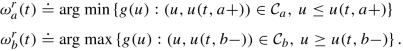
The set of boundary controls (ω _a(t), ω _b(t)) of Theorem 15, which stabilize the system (2.28), in the case u ^∗ < u _m, can be chosen according to the following cases.

• 1. If $\left (u(t,a+), u(t,b-)\right ) \in \left [m, +\infty \right ) \times \left (m, +\infty \right )$, then

  $$\displaystyle \begin{aligned} \omega_a(t) \in \left[m, u(t,a+)\right) \qquad \omega_b(t) = u(t, b-). \end{aligned}$$

• 2. If $\left (u(t,a+), u(t,b-)\right ) \in \left [m, +\infty \right ) \times \left (-\infty , m\right ]$, then

  $$\displaystyle \begin{aligned} \omega_a(t) \in \left(m, +\infty\right) \qquad \omega_b(t) \in \left(-\infty, m\right) \qquad g\left(\omega_a(t)\right) = g\left(\omega_b(t)\right). \end{aligned}$$

• 3. If $\left (u(t,a+), u(t,b-)\right ) \in \left (- \infty , m \right ) \times \left (-\infty , m\right ]$, then

  $$\displaystyle \begin{aligned} \omega_a(t) = u(t, a+) \qquad \omega_b(t) = u^*. \end{aligned}$$

• 4. If $\left (u(t,a+), u(t,b-)\right ) \in \left (- \infty , m \right ) \times \left (m, +\infty \right ]$ and $g\left (u\left (t, a+\right )\right ) < g\left (u\left (t, b-\right )\right )$, then

  $$\displaystyle \begin{aligned} \omega_a(t) = u(t, a+) \qquad \omega_b(t) = u(t, b-). \end{aligned}$$

• 5. If $\left (u(t,a+), u(t,b-)\right ) \in \left (- \infty , m \right ) \times \left (m, +\infty \right ]$ and $g\left (u\left (t, a+\right )\right ) \ge g\left (u\left (t, b-\right )\right )$, then

  $$\displaystyle \begin{aligned} \omega_a(t) = u(t, a+) \qquad \omega_b(t) = u^*. \end{aligned}$$

Remark 4

The boundary controls in Theorem 15 provide Lyapunov stability, but not asymptotic stability in general. In the following section, a greedy controller is defined and it maximizes the instantaneous decrease of the Lyapunov function (but also not guaranteeing asymptotic stability). Finally, in Sect. 2.4.5 we design an improved controller which guarantees asymptotic stability and invariance of the class PWS ⁺.

2.4.4 Greedy Controls

Here we characterize the values of boundary controls, that minimize the derivative of the Lyapunov function V (2.29). Since the type of waves generated at the boundaries influences the value of the derivative of V , we first provide a detailed description of them. Table 2.1 summarizes the types of waves created at the left boundary for controls taking values in the control space $\mathcal {C}_a$; see Definition 3.

Table 2.1 Waves exiting from the left boundary depending from the boundary control and the trace of the solution at this boundary

Let us characterize the changes in the Lyapunov function, due to the variation in the number of shock waves in the solution, resulting both from internal interactions and from the generation or absorption of waves at the boundaries.

Proposition 3

Fix a time $\bar t$ at which the number of jump discontinuities changes.

• 1. If two shock waves interact at time $\bar t$ , then the derivative of the Lyapunov function V decreases, i.e., $V'(\bar t-) > V'(\bar t+)$.

• 2. Assume that a discontinuity wave crosses the left boundary and let us denote u ⁻ the value of the boundary trace at time $\bar t-$ and u ⁺ the value of the boundary trace at time $\bar t+$ . The jump in the derivative of the Lyapunov function reads

  $$\displaystyle \begin{aligned} V'(\bar t+) - V' (\bar t-) = \left(f(u^{+}) - f(u^{-})\right) \,\left(\frac{{u}^{-} + {u}^{+}}{2} - u^*\right), \end{aligned} $$

  (2.35)

  where the term $\left (f(u^{+})-f(u^{-})\right )$ is positive, since f is a convex flux. Moreover we have the following cases.

  • (a) If $u^{*} < \frac {u^{-} + u^{+}}{2}$ , then there is an increase in the derivative of the Lyapunov function V .

  • (b) If $u^{*} > \frac {u^{-}+u^{+}}{2}$ , then there is a decrease in the derivative of the Lyapunov function V .

  The case of right boundary can be treated similarly with a change in the sign in (2.35).

For a proof see [40, Proposition 3]. Proposition 3 can be restated in the case of a concave flux function. The next result selects the boundary controls that maximize the decrease rate of the Lyapunov function V in two different cases. In the first one only rarefaction waves are created, while in the second one shock waves are produced.

Proposition 4 ([40, Proposition 4])

Let u be a solution to the initial-boundary value problem (2.28) and let g be the function introduced in (2.34).

• 1. The boundary controls $t \mapsto \omega ^{r}_{a}$ and $t \mapsto \omega ^{r}_{b}$ that minimize the decrease of the Lyapunov function V without introducing shock waves are given by:

  

• 2. The boundary controls $t \mapsto \omega ^{s}_{a}(t)$ and $t \mapsto \omega ^{s}_{b}(t)$ that minimize the decrease of the Lyapunov function V by introducing discontinuities at the boundaries, can be obtained by:

  

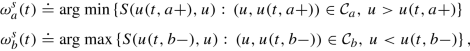
  where

  $$\displaystyle \begin{aligned} S(u, v) := \left(f(v) - f(u)\right) \,\left(\frac{u + v}{2} - u^*\right). \end{aligned}$$

In the case u ^∗ < u _m, a greedy boundary control (ω _a(t), ω _b(t)), maximizing the instantaneous decrease of the Lyapunov function (2.29), can be constructed in the following way; see Fig. 2.2.

Fig. 2.2

Construction of the greedy stabilizing controller for the Burgers flux f(u) = u ² in the case u ^∗ < 0 = u _m. The cases correspond to the ones of the procedure described in Sect. 2.4.4

• Case 1. If $(u(t,a+), u(t,b-)) \in \left [u_m, +\infty \right ) \times \left (u_m, +\infty \right )$, then

  $$\displaystyle \begin{aligned} \omega_a(t) = u_m, \qquad \omega_b(t) = u(t, b-). \end{aligned}$$

• Case 2. If $(u(t,a+), u(t,b-)) \in \left [u_m, +\infty \right ) \times \left (-\infty , u_m\right ]$, then

  $$\displaystyle \begin{aligned} \omega_a(t) = u_m, \qquad \omega_b(t) = u^*. \end{aligned}$$

• Case 3. If $(u(t,a+), u(t,b-)) \in \left (-\infty , u_m \right ) \times \left (-\infty , u_m\right ]$, then

  $$\displaystyle \begin{aligned} \omega_a(t) = u(t, a+), \qquad \omega_b(t) = u^*. \end{aligned}$$

• Case 4. If $(u(t,a+), u(t,b-)) \in \left (-\infty , u_m \right ) \times \left (u_m, +\infty \right )$ and $g\left (u(t, b-)\right ) > g\left (u^*\right )$, then

  $$\displaystyle \begin{aligned} \omega_a(t) = u(t, a+), \qquad \omega_b(t) = u(t, b-). \end{aligned}$$

• Case 5. If $(u(t,a+), u(t,b-)) \in \left (-\infty , u_m \right ) \times \left (u_m, +\infty \right )$ and $g\left (u(t, b-)\right ) \le g\left (u^*\right )$, then

  $$\displaystyle \begin{aligned} \omega_a(t) = u(t, a+), \qquad \omega_b(t) = u^*. \end{aligned}$$

We note in Example 1 that with the greedy controller constructed in this part asymptotic stability may not be obtained. We also illustrate that the naive brute force control (ω _a(t) = u ^∗, ω _b(t) = u ^∗) may create oscillations at the boundary.

Example 1

Choose u ^∗ < u _m and define $\hat u$ by $u_m < \hat {u}$ and $f(\hat {u})=f(u^{*})$. Given 0 <  Δ < (a + b)∕2, such that $\frac {b-a}{4\Delta }\in {\mathbb N}$, and $0<k<\hat {u}$ we consider the following initial datum

$$\displaystyle \begin{aligned} u_{0}(x)= \left\{ \begin{array}{l@{\qquad }l} u_m, & x \in \left(a,\frac{a+b}{2}\right) \\ \hat{u} - k, & x \in \left(\frac{a+b}{2}+(2\,p)\,\Delta,\frac{a+b}{2}+(2\,p+1)\, \Delta\right) \\ & \quad p \in \left\{0,\cdots,\frac{b-a}{4\,\Delta}-1\right\} \\ \hat{u} + k, & x \in \left(\frac{a+b}{2}+(2\,p+1)\,\Delta,\frac{a+b}{2}+(2\,p+2)\, \Delta\right) \\ & \quad p \in \left\{0,\cdots,\frac{b-a}{4\,\Delta}-1\right\}. \end{array} \right. \end{aligned}$$

In such a case, Case 1. applies, hence the boundary controls are (ω _a(t) = u _m, ω _b(t) = u(t, b−)). The characteristic speed of u _m is zero, thus the right boundary value converges toward u _m in infinite time. The solution remains in the configuration characterized by Case 1., and converges to the steady state u _m not reaching the target density u ^∗. This shows that stability is achieved but not asymptotic stability.

The brute force control (ω _a(t) = u ^∗, ω _b(t) = u ^∗) has no action on the system when $u(t,b-) = \hat {u} + k$, since the control values are outside of the control space $\mathcal {C}_b$. While when $u(t,b-) = \hat {u} - k$, the brute force control induces slow backward moving shock waves $(\hat {u} - k, u^{*})$ from the right boundary which interact with fast forward moving shock waves $(\hat {u} + k,\hat {u} - k)$ coming from the initial datum, and create slow forward moving shock waves $(\hat {u} + k,u^{*})$. Hence we observe large oscillations at the right boundary, comparable to the oscillations in the initial datum. More precisely, the trace at the boundary x = b oscillates between the value u ^∗ and values in the interval $[\hat {u}-k,\hat {u}+k]$, generating a total variation in time which satisfies

$$\displaystyle \begin{aligned} \mathrm{TV}_t(u(t,b-))\geq \frac{b-a}{4\Delta}(\hat{u}-k-u^*). \end{aligned}$$

Since Δ is arbitrary, the boundary oscillations can be arbitrarily large, but in any case proportional to the oscillations in the initial datum. Eventually all the waves generating by an oscillating initial datum exit the domain and the naive control produces backward moving shock waves (u _m, u ^∗) which yield convergence.

2.4.5 Lyapunov Asymptotic Stability

Here we design a control strategy, which guarantees Lyapunov asymptotic stability. More precisely, Theorem 16 shows that the associated solution to (2.28) remains in the class PWS ⁺ for initial data u ₀ in the same class. Moreover, in Theorem 17 we state BV estimates for the solution and the boundary controls. Finally, in Theorem 18, we use the BV estimates to extend the construction to BV initial data and we state Lyapunov asymptotic stability.

In this part, we restrict to the case u ^∗ < u _m for simplicity. Define $\hat u > u_m$ by $f(\hat u)=f(u^*)$, $\check {u}> u_m$ by $g(\check {u})=g(u^*)$, and $\bar u = \frac {\hat {u}+\check {u}}{2}$. By Lemma 1, we deduce that $\check {u}<\hat {u}$ and thus $\check {u}<\bar {u}<\hat {u}$. The specific choice of $\bar {u}$ guarantees the decrease of V (⋅) (as it would any other control in $]\check {u}, \hat {u}[$.) The feedback controls ω _a(t), ω _b(t), are defined as:

$$\displaystyle \begin{aligned}~{} \left\{\!\! \begin{array}{l@{\quad }l} \left(u_m, u(t, b-)\right) & \mathrm{if}\, (u(t,a+),u(t,b-)) \in \left[u_m, +\infty \right) \times \left(\bar u, +\infty \right), \\ \left(u_m, u^*\right) & \mathrm{if}\, (u(t,a+),u(t,b-)) \in \left[u_m, +\infty \right) \times \left(-\infty, \bar u \right], \\ \left(u(t, a+), u^*\right) & \mathrm{if}\, (u(t,a+),u(t,b-)) \in \left(-\infty, u_m\right) \times \left(-\infty, \bar u\right], \\ \left(u(t,a+), u(t,b-)\right) & \mathrm{if}\, (u(t,a+),u(t,b-)) \in \left(-\infty, u_m\right) \times \left(\bar u,+\infty\right). \end{array} \right. \end{aligned} $$

(2.36)

Notice that the boundary controls are of feedback type, since they depend only on the trace of the unknown at the boundaries. Instead, the “nonlocal” boundary controls, defined in Sect. 2.4.6, depend also on the initial state.

We have the following result.

Theorem 16

Consider an initial datum u ₀ in PWS ⁺ and the boundary controls given by formula (2.36). Then the corresponding boundary value problem admits a unique solution, which belongs to the class PWS ⁺ for all times. Moreover, the function V (⋅) is strictly decreasing along the solution and the equation is stable in the sense of Lyapunov.

To extend the result to general initial data in BV, we need estimates on the total variation in time of the controls TV_t(ω _a), TV_t(ω _b), and in space of the generated solution TV_x(u(t, ⋅)), which are given by the next result.

Theorem 17

Consider an initial datum u ₀ in PWS ⁺ , the boundary controls given by Case 1. – Case 5. , and let us indicate by u(t, x) the corresponding solution. Then, defining $C=2\,\left (\sup _x |u_0(x) - u_m| +|u_m-u^*|\right )$ , we have the following estimates:

$$\displaystyle \begin{aligned} \mathrm{TV}_x(u(t,\cdot)) & \leq \mathrm{TV}_x(u_0)+C+|\bar{u}-u^*| \end{aligned} $$

(2.37)

$$\displaystyle \begin{aligned} \mathrm{TV}_t(\omega_a) & \leq \mathrm{TV}_x(u_0)+C \end{aligned} $$

(2.38)

$$\displaystyle \begin{aligned} \mathrm{TV}_t(\omega_b) & \leq \mathrm{TV}_x(u_0)+C+|\bar{u}-u^*| \cdot\frac{\mathrm{TV}_x(u_0)+C}{|\bar{u}-\hat{u}|}. \end{aligned} $$

(2.39)

The proof of Theorem 17 is based on careful estimates on the flux variation and possible wave patterns generated by the boundary controls; see [40, Theorem 6]. We are now ready to state the last result of this section [40, Theorem 7].

Theorem 18

Consider an initial datum u ₀ in BV and the boundary controls given by formula (2.36), then there exists a unique entropic solution to the corresponding initial-boundary problem such that (2.37), (2.38) and (2.39) hold true. Moreover, lim_t→+∞ V (t) = 0, i.e. $\lim _{t\to +\infty }\|u(t,\cdot )-u^*\|{ }_{{\mathbf {L}}^{2}}=0$.

To prove Theorem 18, one first uses standard compactness and Helly’s Theorem, then observe that the solution attains the boundary value and, finally, use the decay to N-wave solutions, see [226]. Notice that, because of the BV estimates, the convergence of u actually holds in all L ^p norms.

2.4.6 Nonlocal Controls

As we noticed the greedy control may not stabilize the system to u ^∗, while the brute force control u _a ≡ u _b ≡ u ^∗ may overshoot and produce oscillations. Finally, control (2.36) stabilizes the system, but the stabilization time can be far from optimal. Therefore, in this section, we show nonlocal controls $\omega _{a}^{nl}$ $\omega _{b}^{nl}$, which fast stabilize the system to u ^∗. We use the term nonlocal to indicate that these controls depend not only on the values of the traces u(t, a+) and u(t, b−).

We focus again, for simplicity, only on the case u ^∗ < u _m. Define A =sup_{x ∈ [a,b]} u ₀(x) and $\hat A < u_m$ be such that $f(\hat {A})=f(A)$. For every $U< \hat {A}$ we define:

$$\displaystyle \begin{aligned} T_1(U)=\frac{(b-a)\,(A-U)}{f(U)-f(A)}, \quad T_0(U)=T_1-\frac{(b-a)}{|f'(U)|}\end{aligned} $$

(2.40)

and set $\omega _a^{nl}$ as in (2.36), while:

$$\displaystyle \begin{aligned} \omega_b^{nl}(t)=\left\{ \begin{array}{ll} U, & 0\leq t\leq T_0, \\ u^*, & T_0<t<+\infty. \end{array} \right. \end{aligned} $$

(2.41)

The meaning of such construction is as follows. First, in the same spirit as [149, 150, 179], we send a large shock (u ₀(a+), U) with negative speed to move the system in the zone u < u _m and then apply the stabilizing control. Notice that T ₁ is computed as the maximal time taken by the big shock to cross the interval [a, b], while T ₀ is the time at which the characteristic corresponding to u ^∗ should start from b to reach a at time T ₁. These choices will guarantee the desired effect. Notice also that T ₀ is a safe choice, but smaller values may give a better performance.

2.4.7 Numerical Examples

In this section, we present numerical results obtained for a benchmark scenario. The numerical scheme used here is the standard Godunov scheme [154] with 200 cells in space and a time discretization satisfying the tight Courant-Friedrich-Levy (CFL) condition [216]. We consider the flux function u↦u ²∕2, the equilibrium state u ^∗ = −1, and the space domain [0, 1] with the oscillating initial condition

$$\displaystyle \begin{aligned} u_{0}(x) = 1+ 0.5 \sin{}(20x). \end{aligned} $$

(2.42)

In Fig. 2.3 we present the evolution of the system under four different controllers: the greedy boundary control (defined in Proposition 4), the brute force boundary control u _a = u _b = u ^∗, the stabilizing control (defined in Sect. 2.4.3), and the nonlocal control (formula 2.41) with U = −2 and T ₀ as defined in (2.40). The greedy control allows oscillations to exit from the right boundary but the solution does not converge to the steady state u ^∗ = −1. On the other side the brute force control converges to the steady state but generates oscillations on the right boundary as can be seen in Fig. 2.4, top. The stabilizing control also converges but it is less oscillating with respect to the brute force control. The nonlocal control guarantees convergence and avoids oscillations. The evolution of the solution under the action of the stabilizing control and the brute force control are very similar. The decrease of the corresponding Lyapunov function is represented in Fig. 2.4, bottom. One can note how the nonlocal control decreases much faster than the other methods.

Fig. 2.3

Numerical solution of Burgers equation: Evolution of the solution for the various controllers with oscillating initial data

Fig. 2.4

Downstream trace and Lyapunov functions: the Lyapunov functions for different controls are represented in the bottom subfigure. The downstream boundary are represented in the top subfigure respectively

To study the dependence of the nonlocal control stabilization performance on the parameters U and T ₀ we run several simulations with different values of these parameters, see Fig. 2.5 for U ∈ [−2.1, −1.5] and T ₀ ∈ [0.5, 2]. The convergence time is defined as the first time such that V (t) ≤ 0.1. We notice that longest convergence time corresponds to U = −1.5 and T ₀ = 0.5 while the fastest corresponds to U = −2.1 and T ₀ = 1. Moreover, for each fixed U there exists an optimal switching time T ₀ that minimizes the convergence time.

Fig. 2.5

Convergence time of the Lyapunov function: dependence of the convergence time of the Lyapunov function from U and T ₀. The convergence time is defined as the first time for which V (t) ≤ 0.1

To further illustrate the oscillations of the boundary trace generated by the brute force control we simulated the case in which the initial datum is strongly oscillating:

$$\displaystyle \begin{aligned} u_{0}(x)= 1+ 0.3\sin{}(50x). \end{aligned} $$

(2.43)

In Fig. 2.6 the trace of the brute force control shows, at initial times, one big oscillations and then the oscillations continues until t = 1. For the stabilizing control the oscillations are smaller but they extend for a longer period up to time t = 1.5.

Fig. 2.6

Downstream trace: value of the solution at the right boundary for a strong oscillating initial data

2.5 Mixed Systems PDE-ODE

Here, we present a slightly different system with respect the previous ones of the present Chapter. More precisely, we consider a system of balance laws (PDE) with boundary, coupled with a system of ordinary differential equations (ODE). The coupling condition between the PDE and the ODE is at the level of the boundary. Moreover, we do not consider explicitly a control for such a system. However, the solution to the ODE can be seen as an external control for the system of balance laws. The boundary position for the PDE is not fixed a-priori, but it is given by a function γ, which is the solution to an ordinary differential equation. Therefore, we consider the system of conservation laws (2.1) on the domain $\mathcal {D} = \left \{\left (t, x\right ): t \ge 0, \, x \ge \gamma (t)\right \}$. We present both the mathematical description and a theoretical result about existence of solutions for the Cauchy problem.

Let us consider the following mixed ODE-PDE systems:

$$\displaystyle \begin{aligned} \left\{ \begin{array}{l@{\qquad }l} \partial_t u + \partial_x f(u ) = g(u ), & x > \gamma(t), t > 0, \\ b \left( u \left(t,\gamma(t)+ \right) \right) = B \left( t, w(t) \right), & t > 0, \\ \dot w = F \left( t, u \left(t,\gamma(t)+ \right) , w(t)\right), & t > 0, \\ \dot{\gamma}(t) = \Pi \left( w(t) \right), & t > 0. \end{array} \right. \end{aligned} $$

(2.44)

Here the unknowns are u = u(t, x), w = w(t), and γ = γ(t). As said before, the function u is defined for t ≥ 0 and x ≥ γ(t), while w and γ are defined for t ≥ 0. We assume the following hypotheses.

(MS.1) :

$\Omega \subseteq \mathbb {R}^n$ is an open set. Moreover $\hat u \in \Omega$, $\hat w \in \mathbb {R}^m$ and $\hat x \in \mathbb {R}$. For δ > 0, define the sets

$$\displaystyle \begin{aligned} \mathcal{V} & = \left\{ u \in \hat u + (\mathbf{BV} \cap {\mathbf{L}}^{1}) (\mathbb{R};\mathbb{R}^n) \colon u (\mathbb{R}) \subset \Omega \right\}, \\ \mathcal{V}_\delta & = \left\{ u \in \mathcal{V} \colon \mathrm{TV}(u ) \leq \delta \right\}. \end{aligned} $$

(MS.2) :

The flux function $f:\Omega \to \mathbb {R}^n$ is smooth. Moreover the system of balance laws is strictly hyperbolic with each characteristic field either genuinely nonlinear or linearly degenerate.

(MS.3) :

For δ > 0, the source function $g \colon \mathcal {V}_{\delta } \to {\mathbf {L}}^{1}(\mathbb {R}; \mathbb {R}^n)$ satisfies, for suitable L ₁, L ₂ > 0, the estimates

$$\displaystyle \begin{aligned} \left\| g(u ) - g(u ') \right\|{}_{{\mathbf{L}}^{1}} \leq L_1 \left\| u -u ' \right\|{}_{{\mathbf{L}}^{1}} \quad \mbox{ and } \quad \mathrm{TV} \left(g(u)\right) \leq L_2 \,, \end{aligned}$$

for every $u ,u ' \in \mathcal {V}_{\delta }$.

(MS.4) :

$\Pi \in {\mathbf {C}}^{0,1}(\mathbb {R}^m; \mathbb {R})$.

(MS.5) :

There exist c > 0 and p ∈{1, 2, …, n − 1} such that $\lambda _p(\hat u )< \Pi (\hat w) - c$ and $\lambda _{p+1}(\hat u ) > \Pi (\hat w) + c$.

(MS.6) :

$b \in {\mathbf {C}}^{1}(\Omega ; \mathbb {R}^{n-p})$ is such that

$$\displaystyle \begin{aligned} \det \left( D_u b(\hat u ) \left[ r_{p+1}(\hat u ) \quad r_{p+2}(\hat u ) \quad \cdots \quad r_{n}(\hat u ) \right] \right) \neq 0. \end{aligned}$$

(MS.7) :

The map $F \colon \mathbb {R}^+ \times \Omega \times \mathbb {R}^m \longrightarrow \mathbb {R}^m$ is such that:

• (a) for all u ∈ Ω and $w \in \mathbb {R}^m$, the function t↦F(t, u, w) is Lebesgue measurable;

• (b) for all compact subset K of $\Omega \times \mathbb {R}^m$, there exists C _K > 1 such that, for all $t \in \mathbb {R}^+$ and (u ₁, w ₁), (u ₂, w ₂) ∈ K,

  $$\displaystyle \begin{aligned} \left\| F(t,u _1,w_1) - F(t,u _2,w_2) \right\|{}_{\mathbb{R}^m} \leq C_K \, \left( \left\| u _1 - u _2 \right\|{}_{\mathbb{R}^n} + \left\| w_1 - w_2 \right\|{}_{\mathbb{R}^m} \right); \end{aligned}$$

• (c) there exists a function $C \in {\mathbf {L}}_{\mathrm {loc}}^1(\mathbb {R}^+; \mathbb {R}^+)$ such that, for all t > 0, u ∈ Ω and $w \in \mathbb {R}^m$,

  $$\displaystyle \begin{aligned} \left\| F(t,u ,w) \right\|{}_{\mathbb{R}^m} \leq C(t) \, \left(1 + {\left\| w \right\|}_{\mathbb{R}^m}\right) \,. \end{aligned}$$

(MS.8) :

$B \in C^1(\mathbb {R}^+ \times \mathbb {R}^m; \mathbb {R}^{n - p})$ is locally Lipschitz, i.e., for every compact subset K of $\mathbb {R}^m$, there exists a constant $\tilde C_K > 0$ such that, for every t > 0 and w ∈ K:

$$\displaystyle \begin{aligned} \left\| \frac{\partial}{\partial t} B(t,w) \right\|{}_{\mathbb{R}^{n-p}} + \left\| \frac{\partial}{\partial w} B(t,w) \right\|{}_{\mathbb{R}^{n-p}} \leq \tilde C_K \,. \end{aligned}$$

Remark 5

Condition (MS.5) is analogous to the non-characteristic condition (NC) in the case of moving boundary. This is strictly related to conditions (MS.6) and (MS.8), describing how boundary conditions are assigned; see also [5,6,7].

Now we introduce the definition of solution for (2.44).

Definition 4

Let T > 0. A triple (u, w, γ) with

$$\displaystyle \begin{aligned} u \in {\mathbf{C}}^{0}\left( [0,T]; \mathcal{V} \right) \qquad w \in {\mathbf{W}}^{1, 1}\left([0,T] ;\mathbb{R}^m\right) \qquad \gamma \in {\mathbf{W}}^{1, \infty} \left([0, T] ;\mathbb{R}^m\right) \end{aligned}$$

is a solution to (2.44) on [0, T] with initial datum (u ₀, w ₀, x ₀) such that $u _0 \in \mathcal {V}$ with $u _0(x) = \hat u$ for x < x ₀, $w_0 \in \mathbb {R}^m$ and $x_0 \in \mathbb {R}$, if

• 1. u is an entropy admissible solution to

  $$\displaystyle \begin{aligned} \left\{ \begin{array}{l@{\qquad }l} \partial_t u + \partial_x f(u ) = g(u ), & x > \gamma_\ast (t),\, t > 0, \\ b \left( u \left(t,\gamma_\ast (t)+ \right) \right) = B_* \left(t\right), & t > 0, \end{array} \right. \end{aligned}$$

  on [0, T] with $B_*(t) = B\left (t, w(t)\right )$, γ _∗(t) = γ(t), and initial datum u ₀;

• 2. w solves

  $$\displaystyle \begin{aligned} \left\{ \begin{array}{l@{\qquad }l} \dot w = F_* ( t, w), & t > 0, \\ w(0) = w_0, \end{array} \right. \end{aligned}$$

  on [0, T] with $F_*(t) = F\left (t,u \left (t,\gamma (t)+\right ), w \right )$ a.e.;

• 3. $\displaystyle \gamma (t) = x_0 + \int _0^t \Pi \left ( w(\tau )\right ) \,\mathrm {d}\tau$ for a.e. t ∈ [0, T].

The following result holds; for a proof see [42].

Theorem 19

Let (MS.1) – (MS.8) hold. Assume that $b(\hat u ) = B(0,\hat w)$ . Then, there exist positive constants δ, Δ, L, T _δ , domains $\widehat {\mathcal {D}}_t$ (for t ∈ [0, T _δ]), and maps

$$\displaystyle \begin{aligned} \widehat P(t,t_0) \colon \widehat {\mathcal{D}}_{t_0} \to \widehat {\mathcal{D}}_{t_0 + t}, \end{aligned}$$

defined for t ₀, t ₀ + t ∈ [0, T _δ], such that

• 1. $\left ( \mathcal {V}_{\delta } \times B_{\delta } (\hat w) \times \left ]\hat x -\delta , \hat x + \delta \right [ \right ) \subseteq \widehat {\mathcal {D}}_t \subseteq \left ( \mathcal {V}_{\Delta } \times B_\Delta (\hat w) \times \left ]\hat x - \Delta , \hat x + \Delta \right [ \right )$ , where the notation $B_r(\hat w)$ denotes the ball of radius r centered at $\hat w$;

• 2. for all t ₀, t ₁, t ₂ with t ₀ ∈ [0, T _δ[, t ₁ ∈ [0, T _δ − t ₀[ and t ₂ ∈ [0, T − t ₀ − t ₁], we have

  $$\displaystyle \begin{aligned} \widehat P(t_2, t_0 + t_1) \circ \widehat P(t_1, t_0) = \widehat P(t_1+t_2, t_0) \qquad \mathrm{and} \qquad \widehat P(0,t_0) = Id; \end{aligned}$$

• 3. for t ₀ ∈ [0, T _δ[, t ∈ [0, T _δ − t ₀], and $(u ,w,x), (\bar u ,\bar w, \bar x) \in \widehat {\mathcal {D}}_{t_0}$

  $$\displaystyle \begin{aligned} & \left\| \widehat P(t,t_0)(u ,w,x) - \widehat P(t,t_0)(\bar u ,\bar w, \bar x) \right\| _{{\mathbf{L}}^{1}\times \mathbb{R}^m \times \mathbb{R}} \\ & \le L \left( \left\| u - \bar u \right\|{}_{{\mathbf{L}}^{1}} + \left\| w - \bar w \right\|{}_{\mathbb{R}^m} + \left\vert x - \bar x \right\vert \right); \end{aligned} $$

• 4. for all $(u _0, w_0, x_0) \in \widehat {\mathcal {D}}_0$ , the map $t \mapsto \widehat P(t,0)(u _0,w_0, x_0)$ , defined for t ∈ [0, T _δ], solves (2.44) in the sense of Definition 4.

2.5.1 Examples

We consider here several examples of applications of Theorem 19. In Example 2, we consider the case of a tube with a piston filled with gas, in Example 3 a sewer system with a vertical manhole is considered, in Example 4 we present a system describing a portion of the circulatory system, while in Example 5 the case of a solid body in a fluid is considered.

Example 2

Consider a tube filled with fluid and closed to the left by a piston. The gas dynamics can be described by the p-system in the Lagrangian coordinates, coupled with an ordinary differential equation governing the piston’s evolution. More precisely

$$\displaystyle \begin{aligned} \left\{ \begin{array}{l} \partial_t \tau - \partial_x v =0 \\ \partial_t v + \partial_x p(\tau) =0 \\ V = v(t,0+) \\ \dot V = \alpha \cdot \left( P(t) - p\left(\tau(t,0+)\right) \right), \end{array} \right. \end{aligned} $$

(2.45)

where t is time, x the Lagrangian coordinate (i.e., represent the position of gas particles in the original frame), τ the specific volume, v the Lagrangian speed of the flow, p the pressure in the fluid, V the speed of the piston, P(t) the pressure to the left of the piston, and α is the ratio between the section of the tube and the mass of the piston. The acceleration of the piston is due to the difference between the pressure of the fluid and that of the outer environment. The problem (2.45) can be written in the form (2.44) and, under suitable assumptions, Theorem 19 can be applied.

Example 3

Consider a sewer network composed by a single junction, located at x = 0, that joins k horizontal pipes to one vertical manhole. The flow in the i-th tube, for i = 1, ⋯ , n, can be described by the Saint Venant equations (see [199, formula (108.1)] and Example 8)

$$\displaystyle \begin{aligned} \left\{ \begin{array}{l} \partial_t A_i + \partial_x Q_i = 0 \\ \partial_t Q_i + \partial_x \left(\frac{Q_i^2}{A_i}+p_i(A_i)\right) = 0 \end{array} \right. \end{aligned}$$

ensuring the conservation of mass and momentum. The quantity A _i is the wet cross sectional area, Q _i the flow in the x direction, and p _i is a function representing the hydrostatic pressure. The complete system, which falls within the class (2.44), is

$$\displaystyle \begin{aligned} \left\{ \begin{array}{l@{\qquad }l} \displaystyle \partial_t A_i + \partial_x Q_i = 0, & i=1, \cdots, n, \\ \displaystyle \partial_t Q_i + \partial_x \left(\frac{Q_i^2}{A_i}+p_i(A_i)\right) = 0, & i=1, \cdots, n, \\ \displaystyle \hat h(t) = \frac{1}{2g} \frac{Q_i(t, 0+)^2}{A_i(t, 0+)^2} + h_i \left(A_i(t, 0+)\right), & i=1, \cdots, n \\ \displaystyle h_M(t) = - \frac{1}{2g \, A_M^2} \left(\sum_{i=1}^k Q_i(t, 0+)\right) \left\vert \sum_{i=1}^k Q_i(t, 0+) \right\vert + \hat h(t), \\ \displaystyle \dot{h}_M(t) = \frac{1}{A_M} \left( Q_{\mbox{ext}}(t) - \sum_{i=1}^k Q_i(t, 0+)\right), \end{array} \right. \end{aligned} $$

(2.46)

where we require, as boundary condition, the equality of all the hydraulic heads $\hat h$ at the junction, and the height h _M of the water inside the manhole is determined by the last two equations of (2.46) based on the conservation of the total amount of water.

Example 4

Following [129, formulæ (2.3), (2.12), (2.14)], [133] and [62], we consider the 1D model for blood flowing through an artery, coupled with a 0D model describing the averaged mass and flow rate in a given terminal compartment of the circulatory system (e.g., capillary bed, venous circulation). The complete model is

$$\displaystyle \begin{aligned} \left\{ \begin{array}{l} \partial_t a + \partial_x q = 0 \\ \partial_t q + \partial_x \left( \alpha \frac{q^2}{a} + \frac{1}{\rho}\pi(a) \right) = -2\frac{\alpha}{\alpha-1}\nu\frac{q}{a} \\ a(t,0+) = a_0\left( 1 + \frac{p - p_{ref}}{\beta} \right)^2 \\ \dot P = - \frac{1}{C} Q + \frac{1}{C} q(t,0) \\ \dot Q = - \frac{R}{L}Q + \frac{1}{L} P - \frac{1}{L} P(t,l), \end{array} \right. \end{aligned} $$

(2.47)

where ρ is the blood density, q is the arterial flow rate, a denotes the arterial cross section, p(a) is the arterial blood pressure, $\pi (a) = \int _{a_0}^a \tilde {a} \, p'(\tilde {a}) \,\mathrm {d}\tilde {a}$, and P and Q denote respectively the compartmental mean blood pressure and the compartmental mean flow rate. The remaining constant are:

$$\displaystyle \begin{aligned} \begin{array}{@{}lrl@{\qquad }rl@{}} & a_0 & \text{reference cross section,} & \nu & \text{viscosity coefficient,} \\ & \alpha & \text{Coriolis coefficient,} & \beta & \text{arterial wall elasticity,} \\ & R &\text{ compartmental resistance,} & C & \text{compartmental capacitance,} \\ & L & \text{compartmental inductance.} & & \end{array} \end{aligned}$$

System (2.47) is of type (2.44).

Example 5

We consider the following model describing the evolution of a solid body, locate at position γ(t), inside a compressible fluid, described by the classical p-system (see Example 7):

$$\displaystyle \begin{aligned} \left\{ \begin{array}{l@{\quad }l} \displaystyle \partial_t \rho + \partial_x q = 0, & x \ne \gamma(t),\, t > 0, \\ \displaystyle \partial_t q + \partial_x \left( \frac{{q}^2}{\rho} +p (\rho) \right) = -g\, \rho, & x \ne \gamma (t),\, t > 0, \\ \displaystyle \frac{q\left(t, \gamma(t)-\right)}{\rho\left(t, \gamma(t)-\right)} = \displaystyle \frac{q\left(t, \gamma(t)+\right)}{\rho\left(t, \gamma(t)+\right)} = V, & t > 0, \\ \displaystyle \dot V = -g - \frac{ p\left(\rho \left(t, \gamma(t)+\right)\right) - p\left(\rho \left(t, \gamma(t)-\right)\right)}{m}, & t > 0, \\ \dot{\gamma} (t) = V, & t> 0. \end{array} \right. \end{aligned} $$

(2.48)

The quantities ρ and q are the fluid mass and linear momentum density above and below the particle, p = p(ρ) is the pressure law, V is the speed of the particle located at γ(t) and m is its mass, g is gravity. System (2.48) is a particular case of (2.44).

2.6 Bibliographical Notes

Several papers are concerned with the boundary control of the viscous Burgers equation $\partial _t u + \partial _x \left (\frac {u^2}{2} \right ) = \partial _{xx} u$; see [59, 60, 85, 119, 135, 136, 192, 195, 204, 229, 256]. Given a final time T > 0, an initial condition u ₀ and boundary controls ω _a, ω _b, the control system is

$$\displaystyle \begin{aligned} \left\{ \begin{array}{l} \partial_t u + \partial_x \left(\frac{u^2}{2}\right) = \partial_{xx} u \\ u(0, x) = u_0(x) \\ u(t, a) = \omega_a(t) \\ u(t, b) = \omega_b(t). \end{array} \right. \end{aligned} $$

(2.49)

When the control acts on a single side (i.e., when ω _a or ω _b is a given preassigned function), there are several results concerning the non-controllability of the system. First, Díaz in [119] proved, using a topological argument, that it is not possible to find a solution u to (2.49), which is arbitrary close to certain open subsets of L ²(a, b); see also [135]. In such a case, also the property of exact null controllability does not hold. This means that, for specific initial data u ₀, the final profile u(T, ⋅) cannot be constantly equal to 0. In such direction, Fernández-Cara and Guerrero in [130] gave sharp estimates of the minimal time, which depends on the L ² norm of the initial datum, for which the null controllability property is ensured. Moreover Coron in [86] proved the existence of a time T > 0 sufficiently big such that the system (2.49) is null controllable when ω _a (or ω _b) is constantly equal to 0; see also [69].

In case the control acts on both sides, Fursikov and Imanuvilov in [135] proved that every steady state solution can be reached, provided the final time is sufficiently large, whereas Coron in [86] proved that the system can be driven from the null function to every large constant state; see also [151]. In the presence of an additional distributed control, Chapouly in [69] proved the global controllability property for the viscous Burgers’ equation; see also [1, 13, 19, 219, 240].

In the case of smooth solutions for general systems of balance laws, problems of exact boundary controllability and of asymptotic stabilization have been addressed. These results were obtained by using explicit formulas for the evolution of the Riemann invariants along characteristics; see [34, 110, 161, 215, 217, 218].

Lyapunov methods for stabilizing classical solutions of 2 × 2 systems with characteristics speeds of constant opposite sign have been introduced in [90, 122, 241]. Similar work on boundary damping techniques with applications to the Saint-Venant equations has been proposed in [110, 244]. Lyapunov methods for stabilization in the case of solutions with a finite number of shocks are considered in [40]. In the case of hybrid dynamics, see [9].

Mixed systems, composed by hyperbolic conservation laws and ordinary differential equations interacting at the level of the boundary, have been considered in [18, 41,42,43,44]. Existence of a solution with the vanishing viscosity approach has been studied in [75].

References

Adimurthi, S. Ghoshal, and G. Veerappa Gowda. Exact controllability of scalar conservation laws with strict convex flux. Mathematical Control and Related Fields, 4(4):401–449, 2014. cited By 15.
D. Amadori. Initial-boundary value problems for nonlinear systems of conservation laws. NoDEA: Nonlinear Differential Equations and Applications, 4(1):1–42, 1997.
D. Amadori and R. Colombo. Continuous dependence for 2 × 2 conservation laws with boundary. Journal of Differential Equations, 138(2):229–266, 1997.
D. Amadori and R. Colombo. Viscosity solutions and standard Riemann semigroup for conservation laws with boundary. Rendiconti del Seminario Matematico della Universita di Padova, 99:219–245, 1998.
S. Amin, F. Hante, and A. Bayen. On stability of switched linear hyperbolic conservation laws with reflecting boundaries. Hybrid System: Computation and Control, Lecture Notes in Computer Science, 4981:602–605, 2008, https://doi.org/10.1007/978-3-540-78929-1_44.
F. Ancona and G. Coclite. On the attainable set for Temple class systems with boundary controls. SIAM J. Control Optim., 43(6):2166–2190 (electronic), 2005.
F. Ancona and A. Marson. On the attainable set for scalar nonlinear conservation laws with boundary control. SIAM J. Control Optim., 36(1):290–312 (electronic), 1998.
B. Andreianov, C. Donadello, S. S. Ghoshal, and U. Razafison. On the attainable set for a class of triangular systems of conservation laws. J. Evol. Equ., 15(3):503–532, 2015.
B. Andreianov, F. Lagoutière, N. Seguin, and T. Takahashi. Well-posedness for a one-dimensional fluid-particle interaction model. SIAM J. Math. Anal., 46(2):1030–1052, 2014.
B. Andreianov, S. Sundar Ghoshal, and K. Koumatos. Non-controllability of the viscous Burgers equation and a detour into the well-posedness of unbounded entropy solutions to scalar conservation laws. working paper or preprint, Mar. 2020.
A. Balogh and M. Krstic. Infinite dimensional backstepping-style feedback transformations for a heat equation with an arbitrary level of instability. European journal of control, 8(2):165–175, 2002.
G. Bastin and J.-M. Coron. Stability and Boundary Stabilisation of 1-D Hyperbolic Systems. Number 88 in Progress in Nonlinear Differential Equations and Their Applications. Springer International, 2016.
G. Bastin and J.-M. Coron. A quadratic Lyapunov function for hyperbolic density-velocity systems with nonuniform steady states. Systems & Control Letters, 104:66–71, 2017.
G. Bastin, J.-M. Coron, and B. d’Andréa Novel. On Lyapunov stability of linearised Saint-Venant equations for a sloping channel. Netw. Heterog. Media, 4(2):177–187, 2009.
G. Bastin, J.-M. Coron, A. Hayat, and P. Shang. Exponential boundary feedback stabilization of a shock steady state for the inviscid Burgers equation. Math. Models Methods Appl. Sci., 29(2):271–316, 2019.
S. Blandin, X. Litrico, M. L. Delle Monache, B. Piccoli, and A. Bayen. Regularity and Lyapunov stabilization of weak entropy solutions to scalar conservation laws. IEEE Trans. Automat. Control, 62(4):1620–1635, 2017.
R. Borsche, R. M. Colombo, and M. Garavello. On the coupling of systems of hyperbolic conservation laws with ordinary differential equations. Nonlinearity, 23(11):2749–2770, 2010.
R. Borsche, R. M. Colombo, and M. Garavello. Mixed systems: ODEs - balance laws. J. Differential Equations, 252(3):2311–2338, 2012.
R. Borsche, R. M. Colombo, and M. Garavello. On the interactions between a solid body and a compressible inviscid fluid. Interfaces Free Bound., 15(3):381–403, 2013.
R. Borsche, R. M. Colombo, M. Garavello, and A. Meurer. Differential equations modeling crowd interactions. J. Nonlinear Sci., 25(4):827–859, 2015.
D. M. Bošković, A. Balogh, and M. Krstić. Backstepping in infinite dimension for a class of parabolic distributed parameter systems. Math. Control Signals Systems, 16(1):44–75, 2003.
A. Bressan and G. M. Coclite. On the boundary control of systems of conservation laws. SIAM J. Control Optim., 41(2):607–622, 2002.
J. Burns and S. Kang. A control problem for Burgers equation with bounded input/output. Nonlinear Dynamics, 2(4):235–262, 1991.
C. Byrnes, D. Gilliam, and V. Shubov. On the global dynamics of a controlled viscous Burgers equation. Journal of Dynamical and Control Systems, 4(4):457–519, 1998.
S. Čanić and E. H. Kim. Mathematical analysis of the quasilinear effects in a hyperbolic model blood flow through compliant axi-symmetric vessels. Math. Methods Appl. Sci., 26(14):1161–1186, 2003.
M. Chapouly. Global controllability of nonviscous and viscous Burgers-type equations. SIAM J. Control Optim., 48(3):1567–1599, 2009.
G. M. Coclite and M. Garavello. Vanishing viscosity for mixed systems with moving boundaries. J. Funct. Anal., 264(7):1664–1710, 2013.
J.-M. Coron. Global asymptotic stabilization for controllable systems without drift. Math. Control Signals Systems, 5(3):295–312, 1992.
J.-M. Coron. Some open problems in control theory. In Differential geometry and control (Boulder, CO, 1997), volume 64 of Proc. Sympos. Pure Math., pages 149–162. Amer. Math. Soc., Providence, RI, 1999.
J.-M. Coron. Some open problems on the control of nonlinear partial differential equations. In Perspectives in nonlinear partial differential equations, volume 446 of Contemp. Math., pages 215–243. Amer. Math. Soc., Providence, RI, 2007.
J.-M. Coron and G. Bastin. Dissipative boundary conditions for one-dimensional quasi-linear hyperbolic systems: Lyapunov stability for the C 1-norm. SIAM Journal on Control and Optimization, 53(3):1464–1483, 2015.
J.-M. Coron, G. Bastin, and B. d’Andréa Novel. Dissipative boundary conditions for one-dimensional nonlinear hyperbolic systems. SIAM J. Control Optim., 47(3):1460–1498, 2008.
J.-M. Coron and B. d’Andréa Novel. Stabilization of a rotating body beam without damping. IEEE Trans. Automat. Control, 43(5):608–618, 1998.
J.-M. Coron, B. d’Andrea-Novel, and G. Bastin. A strict Lyapunov function for boundary control of hyperbolic systems of conservation laws. IEEE Transactions on Automatic Control, 52(1):2–11, 2007.
J.-M. Coron, S. Ervedoza, S. S. Ghoshal, O. Glass, and V. Perrollaz. Dissipative boundary conditions for 2 × 2 hyperbolic systems of conservation laws for entropy solutions in BV. J. Differential Equations, 262(1):1–30, 2017.
J.-M. Coron and A. Hayat. PI controllers for 1-D nonlinear transport equation. working paper or preprint, 2018.
J.-M. Coron and H.-M. Nguyen. Dissipative boundary conditions for nonlinear 1-D hyperbolic systems: sharp conditions through an approach via time-delay systems. SIAM J. Math. Anal., 47(3):2220–2240, 2015.
C. M. Dafermos. Generalized characteristics and the structure of solutions of hyperbolic conservation laws. Indiana Univ. Math. J., 26(6):1097–1119, 1977.
C. M. Dafermos. Hyperbolic conservation laws in continuum physics, volume 325 of Grundlehren der Mathematischen Wissenschaften [Fundamental Principles of Mathematical Sciences]. Springer-Verlag, Berlin, second edition, 2005.
J. de Halleux, C. Prieur, J.-M. Coron, B. d’Andréa Novel, and G. Bastin. Boundary feedback control in networks of open channels. Automatica J. IFAC, 39(8):1365–1376, 2003.
F. Di Meglio, R. Vazquez, and M. Krstic. Stabilization of a system of n + 1 coupled first-order hyperbolic linear PDEs with a single boundary input. IEEE Trans. Automat. Control, 58(12):3097–3111, 2013.
J. I. Diaz. Obstruction and some approximate controllability results for the Burgers equation and related problems. In Control of partial differential equations and applications (Laredo, 1994), volume 174 of Lecture Notes in Pure and Appl. Math., pages 63–76. Dekker, New York, 1996.
M. Dick, M. Gugat, and G. Leugering. Classical solutions and feedback stabilization for the gas flow in a sequence of pipes. Networks & Heterogeneous Media, 5(4):691, 2010.
V. Dos Santos, G. Bastin, J.-M. Coron, and B. d’Andréa-Novel. Boundary control with integral action for hyperbolic systems of conservation laws: Stability and experiments. Automatica, 44(5):1310–1318, 2008.
M. A. Fernández, V. Milišić, and A. Quarteroni. Analysis of a geometrical multiscale blood flow model based on the coupling of ODEs and hyperbolic PDEs. Multiscale Model. Simul., 4(1):215–236, 2005.
E. Fernández-Cara and S. Guerrero. Remarks on the null controllability of the Burgers equation. C. R. Math. Acad. Sci. Paris, 341(4):229–232, 2005.
L. Formaggia, A. Quarteroni, and A. Veneziani. The circulatory system: from case studies to mathematical modeling. In Complex systems in biomedicine, pages 243–287. Springer Italia, Milan, 2006.
A. V. Fursikov and O. Y. Imanuvilov. On controllability of certain systems simulating a fluid flow. In Flow control (Minneapolis, MN, 1992), volume 68 of IMA Vol. Math. Appl., pages 149–184. Springer, New York, 1995.
A. V. Fursikov and O. Y. Imanuvilov. Local exact controllability of the Navier-Stokes equations. C. R. Acad. Sci. Paris Sér. I Math., 323(3):275–280, 1996.
O. Glass. On the controllability of the 1-d isentropic euler equation. J. Eur. Math. Soc.(JEMS), 9(3):427–486, 2007.
O. Glass. On the controllability of the non-isentropic 1-d euler equation. Journal of Differential Equations, 257(3):638–719, 2014.
O. Glass and S. Guerrero. On the uniform controllability of the Burgers equation. SIAM J. Control Optim., 46(4):1211–1238, 2007.
S. K. Godunov. A difference method for numerical calculation of discontinuous solutions of the equations of hydrodynamics. Mat. Sb. (N.S.), 47 (89):271–306, 1959.
J. M. Greenberg and T. Li. The effect of boundary damping for the quasilinear wave equation. J. Differential Equations, 52(1):66–75, 1984.
M. Gugat and G. Leugering. Global boundary controllability of the Saint-Venant system for sloped canals with friction. In Annales de l’Institut Henri Poincare, volume 26, pages 257–270. Elsevier, 2009.
M. Gugat, G. Leugering, S. Tamasoiu, and K. Wang. H 2-stabilization of the isothermal Euler equations: a Lyapunov function approach. Chinese Annals of Mathematics, Series B, 33(4):479–500, 2012.
J. K. Hale, S. M. V. Lunel, L. S. Verduyn, and S. M. V. Lunel. Introduction to functional differential equations, volume 99. Springer Science & Business Media, 1993.
A. Hayat. Boundary Stability of 1-D Nonlinear Inhomogeneous Hyperbolic Systems for the C 1 Norm. SIAM Journal on Control and Optimization, 57(6):3603–3638, 2019.
A. Hayat and P. Shang. A quadratic Lyapunov function for Saint-Venant equations with arbitrary friction and space-varying slope. Automatica J. IFAC, 100:52–60, 2019.
T. Horsin. On the controllability of the Burgers equation. ESAIM Control Optim. Calc. Var., 3:83–95, 1998.
L. Hu, F. Di Meglio, R. Vazquez, and M. Krstic. Control of homodirectional and general heterodirectional linear coupled hyperbolic PDEs. IEEE Trans. Automat. Control, 61(11):3301–3314, 2016.
T. Kobayashi. Adaptive regulator design of a viscous Burgers system by boundary control. IMA Journal of Mathematical Control and Information, 18(3):427, 2001.
M. Krstic. On global stabilization of Burgers equation by boundary control. Systems and Control Letters, 37(3):123–141, 1999.
M. Krstic and A. Smyshlyaev. Backstepping boundary control for first-order hyperbolic PDEs and application to systems with actuator and sensor delays. Systems Control Lett., 57(9):750–758, 2008.
M. Krstic and A. Smyshlyaev. Boundary Control of PDEs: A Course on Backstepping Designs, volume 16 of Advances in Design and Control. Society for Industrial and Applied Mathematics (SIAM), Philadelphia, PA, 2008.
L. D. Landau and E. M. Lifschitz. Lehrbuch der theoretischen Physik (“Landau-Lifschitz”). Band VI. Akademie-Verlag, Berlin, fifth edition, 1991. Hydrodynamik. [Hydrodynamics], Translated from the Russian by Wolfgang Weller and Adolf Kühnel, Translation edited by Weller and with a foreword by Weller and P. Ziesche.
M. Leautaud. Uniform controllability of scalar conservation laws in the vanishing viscosity limit. SIAM Journal on Control and Optimization, 50(3):1661–1699, 2012.
P. LeFloch. Explicit formula for scalar nonlinear conservation laws with boundary condition. Math. Methods Appl. Sci., 10(3):265–287, 1988.
G. Leugering and E. J. P. G. Schmidt. On the modelling and stabilization of flows in networks of open canals. SIAM J. Control Optim., 41(1):164–180, 2002.
R. Leveque. Finite volume methods for hyperbolic problems. Cambridge University Press, Cambridge, UK, 2002.
T. Li. Exact boundary controllability of unsteady flows in a network of open canals. In Differential equations & asymptotic theory in mathematical physics, volume 2 of Ser. Anal., pages 310–329. World Sci. Publ., Hackensack, NJ, 2004.
T. Li. Exact boundary controllability of unsteady flows in a network of open canals. Math. Nachr., 278(3):278–289, 2005.
T. Li and L. Yu. Local exact boundary controllability of entropy solutions to linearly degenerate quasilinear hyperbolic systems of conservation laws. ESAIM Control Optim. Calc. Var., 24(2):793–810, 2018.
T. T. Li. Global classical solutions for quasilinear hyperbolic systems, volume 32 of RAM: Research in Applied Mathematics. Masson, Paris; John Wiley & Sons, Ltd., Chichester, 1994.
T. P. Liu. Invariants and asymptotic behavior of solutions of a conservation law. Proc. Amer. Math. Soc., 71(2):227–231, 1978.
H. Ly, K. Mease, and E. Titi. Distributed and boundary control of the viscous Burgers equation. Numerical Functional Analysis and Optimization, 18(1):143–188, 1997.
V. Perrollaz. Exact controllability of scalar conservation laws with an additional control in the context of entropy solutions. SIAM Journal on Control and Optimization, 50(4):2025–2045, 2012.
V. Perrollaz. Asymptotic stabilization of entropy solutions to scalar conservation laws through a stationary feedback law. Ann. Inst. H. Poincaré Anal. Non Linéaire, 30(5):879–915, 2013.
C. Prieur, J. Winkin, and G. Bastin. Robust boundary control of systems of conservation laws. Mathematics of Control, Signals, and Systems, 20(2):173–197, 2008.
T. H. Qin. Global smooth solutions of dissipative boundary value problems for first order quasilinear hyperbolic systems. Chinese Ann. Math. Ser. B, 6(3):289–298, 1985. A Chinese summary appears in Chinese Ann. Math. Ser. A 6 (1985), no. 4, 514.
M. Slemrod. Boundary feedback stabilization for a quasi-linear wave equation. In Control Theory for Distributed Parameter Systems and Applications, pages 221–237. Springer, 1983.
N. Smaoui. Boundary and distributed control of the viscous Burgers equation. Journal of Computational and Applied Mathematics, 182(1):91–104, 2005.
B. Temple. Systems of conversation laws with invariant submanifolds. Transactions of the American Mathematical Society, 280(2):781–795, 1983.
N.-T. Trinh, V. Andrieu, and C.-Z. Xu. Design of integral controllers for nonlinear systems governed by scalar hyperbolic partial differential equations. IEEE Trans. Automat. Control, 62(9):4527–4536, 2017.
Author information
Authors and Affiliations
Rights and permissions
Open Access This chapter is licensed under the terms of the Creative Commons Attribution 4.0 International License (http://creativecommons.org/licenses/by/4.0/), which permits use, sharing, adaptation, distribution and reproduction in any medium or format, as long as you give appropriate credit to the original author(s) and the source, provide a link to the Creative Commons license and indicate if changes were made.
The images or other third party material in this chapter are included in the chapter's Creative Commons license, unless indicated otherwise in a credit line to the material. If material is not included in the chapter's Creative Commons license and your intended use is not permitted by statutory regulation or exceeds the permitted use, you will need to obtain permission directly from the copyright holder.
Copyright information
© 2022 The Author(s)
About this chapter
Cite this chapter
Bayen, A., Monache, M.L.D., Garavello, M., Goatin, P., Piccoli, B. (2022). Boundary Control of Conservation Laws Exhibiting Shocks. In: Control Problems for Conservation Laws with Traffic Applications. Progress in Nonlinear Differential Equations and Their Applications(), vol 99. Birkhäuser, Cham. https://doi.org/10.1007/978-3-030-93015-8_2
Download citation
DOI: https://doi.org/10.1007/978-3-030-93015-8_2
Published:
Publisher Name: Birkhäuser, Cham
Print ISBN: 978-3-030-93014-1
Online ISBN: 978-3-030-93015-8
eBook Packages: Mathematics and StatisticsMathematics and Statistics (R0)