Exponential Stability of Evolutionary Equations

Abstract

In this chapter we study the exponential stability of evolutionary equations. Roughly speaking, exponential stability of a well-posed evolutionary equation

$$\displaystyle \left (\partial _{t,\nu }M(\partial _{t,\nu })+A\right )U=F $$

means that exponentially decaying right-hand sides F lead to exponentially decaying solutions U. The main problem in defining the notion of exponential decay for a solution of an evolutionary equation is the lack of continuity with respect to time, so a pointwise definition would not make sense in this framework. Instead, we will use our exponentially weighted spaces $L_{2,\nu }(\mathbb {R};H)$, but this time for negative ν, and define the exponential stability by the invariance of these spaces under the solution operator associated with the evolutionary equation under consideration.

In this chapter we study the exponential stability of evolutionary equations. Roughly speaking, exponential stability of a well-posed evolutionary equation

$$\displaystyle \begin{aligned} \left(\partial_{t,\nu}M(\partial_{t,\nu})+A\right)U=F \end{aligned}$$

means that exponentially decaying right-hand sides F lead to exponentially decaying solutions U. The main problem in defining the notion of exponential decay for a solution of an evolutionary equation is the lack of continuity with respect to time, so a pointwise definition would not make sense in this framework. Instead, we will use our exponentially weighted spaces $L_{2,\nu }(\mathbb {R};H)$, but this time for negative ν, and define the exponential stability by the invariance of these spaces under the solution operator associated with the evolutionary equation under consideration.

11.1 The Notion of Exponential Stability

Throughout this section, let H be a Hilbert space, $M\colon \operatorname {dom}(M)\subseteq \mathbb {C}\to L(H)$ a material law and $A\colon \operatorname {dom}(A)\subseteq H\to H$ a skew-selfadjoint operator. Moreover, we assume that there exist $\nu _{0}>\mathrm {s}_{\mathrm {b}}\left ( M \right )$ and c > 0 such that

$$\displaystyle \begin{aligned} \operatorname{Re} zM(z)\geqslant c\quad (z\in\mathbb{C}_{\operatorname{Re}\geqslant \nu_{0}}). \end{aligned}$$

By Picard’s theorem (Theorem 6.2.1) we know that for $\nu \geqslant \nu _{0}$ the operator

is causal and independent of the particular choice of ν. We now define the notion of exponential stability.

Definition

We call the solution operators $(S_\nu )_{\nu \geqslant \nu _0}$ exponentially stable with decay rate ρ ₀ > 0 if for all $\rho \in \left [0,\rho _{0}\right )$ and $\nu \geqslant \nu _0$ we have

$$\displaystyle \begin{aligned} S_{\nu}F\in L_{2,-\rho}(\mathbb{R};H)\quad (F\in L_{2,\nu}(\mathbb{R};H)\cap L_{2,-\rho}(\mathbb{R};H)). \end{aligned}$$

Remark 11.1.1

We emphasise that the definition of exponential stability does not mean that the evolutionary equation is just solvable for some negative weights. Indeed, if we consider $H=\mathbb {C}$, A = 0 and M(z) = 1 for $z\in \mathbb {C}$ we obtain that the corresponding evolutionary equation

$$\displaystyle \begin{aligned} \partial_{t,\nu}U=F \end{aligned} $$

(11.1)

is well-posed for each ν≠0. However, we also place a demand for causality on our solution operator. Thus, we only have to consider parameters ν > 0. We obtain the solution U by

$$\displaystyle \begin{aligned} U(t)=\int_{-\infty}^{t}F(s)\,\mathrm{d} s. \end{aligned}$$

As it turns out, the problem (11.1) is not exponentially stable. Indeed, for the solution U is given by

$$\displaystyle \begin{aligned} U(t)=\begin{cases} 0 & \text{ if }t<0,\\ t & \text{ if }0\leqslant t\leqslant1,\\ 1 & \text{ if }t>1, \end{cases} \end{aligned}$$

which does not belong to the space $L_{2,-\rho }(\mathbb {R})$ for any ρ > 0.

We first show that the aforementioned notion of exponential stability also yields a pointwise exponential decay of solutions if we assume more regularity for our source term F.

Proposition 11.1.2

Let $(S_\nu )_{\nu \geqslant \nu _0}$ be exponentially stable with decay rate ρ ₀ > 0, $\nu \geqslant \nu _{0}$, $\rho \in \left [0,\rho _{0}\right )$ and $F\in \operatorname {dom}(\partial _{t,\nu })\cap \operatorname {dom}(\partial _{t,-\rho })$ . Then is continuous and satisfies

$$\displaystyle \begin{aligned} U(t)\mathrm{e}^{\rho t}\to0\quad (t\to\infty). \end{aligned}$$

Proof

We first note that ∂ _t,ν F = ∂ _t,−ρ F by Exercise 11.1. Moreover, since S _ν is a material law operator (i.e., S _ν = S(∂ _t,ν) for some material law S; see Remark 6.3.4) we have

$$\displaystyle \begin{aligned} S_{\nu}\partial_{t,\nu}\subseteq\partial_{t,\nu}S_{\nu}. \end{aligned}$$

Thus, in particular, we have

$$\displaystyle \begin{aligned} S_{\nu}\partial_{t,\nu}F=\partial_{t,\nu}S_{\nu}F=\partial_{t,\nu}U; \end{aligned}$$

that is, $U\in \operatorname {dom}(\partial _{t,\nu })$. Moreover, since $\partial _{t,\nu }F=\partial _{t,-\rho }F\in L_{2,-\rho }(\mathbb {R};H)$, we infer also $U,\partial _{t,\nu }U\in L_{2,-\rho }(\mathbb {R};H)$ by exponential stability. By Exercise 11.1 this yields $U\in \operatorname {dom}(\partial _{t,-\rho })$ with ∂ _t,−ρ U = ∂ _t,ν U. The assertion now follows from the Sobolev embedding theorem (Theorem 4.1.2 and Corollary 4.1.3). □

11.2 A Criterion for Exponential Stability of Parabolic-Type Equations

In this section we will prove a useful criterion for exponential stability of a certain class of evolutionary equations. The easiest example we have in mind is the heat equation with homogeneous Dirichlet boundary conditions, which can be written as an evolutionary equation of the form (cf. Theorem 6.2.4)

in $L_{2,\nu }(\mathbb {R};H)$, where H = L ₂( Ω) ⊕ L ₂( Ω)^d with $\Omega \subseteq \mathbb {R}^{d}$ open, and a ∈ L(L ₂( Ω)^d) with

$$\displaystyle \begin{aligned} \operatorname{Re} a\geqslant c \end{aligned}$$

for some c > 0 which models the heat conductivity, and ν > 0.

Theorem 11.2.1

Let H ₀, H ₁ be Hilbert spaces and $C\colon \operatorname {dom}(C)\subseteq H_{0}\to H_{1}$ a densely defined closed linear operator which is boundedly invertible. Moreover, let M ₀ ∈ L(H ₀) be selfadjoint with

$$\displaystyle \begin{aligned} M_{0}\geqslant c_{0} \end{aligned}$$

for some c ₀ > 0 and $M_{1}\colon \operatorname {dom}(M_{1})\subseteq \mathbb {C}\to L(H_{1})$ be a material law satisfying $\mathrm {s}_{\mathrm {b}}\left ( M_1 \right )< -\rho _1$ for some ρ ₁ > 0 and

$$\displaystyle \begin{aligned} \exists\, c_{1}>0\:\forall z\in\mathbb{C}_{\operatorname{Re}>-\rho_{1}}: \operatorname{Re} M_{1}(z)\geqslant c_{1}. \end{aligned}$$

Then

for each ν > 0. Moreover, for all ν ₀ > 0 the family $(S_\nu )_{\nu \geqslant \nu _0}$ is exponentially stable with decay rate .

In order to prove this theorem we need a preparatory result.

Lemma 11.2.2

Assume the hypotheses of Theorem 11.2.1 . Then for each $z\in \mathbb {C}_{\operatorname {Re}>-\rho _{0}}$ the operator

is boundedly invertible. Moreover,

$$\displaystyle \begin{aligned} \sup_{z\in\mathbb{C}_{\operatorname{Re}\geqslant-\rho}}\left\Vert T(z)^{-1} \right\Vert <\infty \end{aligned}$$

for each ρ < ρ ₀.

Proof

Let $z\in \mathbb {C}_{\operatorname {Re}\geqslant -\rho }$ for some ρ < ρ ₀. We note that M ₁(z) is boundedly invertible with $\left \Vert M_{1}(z)^{-1} \right \Vert \leqslant 1/c_{1}$ (see Proposition 6.2.3(b)) and (C ^∗)⁻¹ = (C ⁻¹)^∗∈ L(H ₀, H ₁) (see Lemmas 2.2.2 and 2.2.9). The beginning of the proof deals with a reformulation of T(z). For this, let u, f ∈ H ₀, v, g ∈ H ₁. Then, by definition, $(u,v)\in \operatorname {dom}(T(z))=\operatorname {dom}(C)\times \operatorname {dom}(C^*)$ and T(z)(u, v) = (f, g) if and only if $v\in \operatorname {dom}(C^*)$ and $u\in \operatorname {dom}(C)$ together with

$$\displaystyle \begin{aligned} zM_0 u - C^*v &= f\\ Cu + M_1 (z)v &=g. \end{aligned} $$

Since both C ^∗ and M ₁(z) are continuously invertible, we obtain equivalently $u\in \operatorname {dom}(C)$ together with

$$\displaystyle \begin{aligned} z(C^*)^{-1}M_0 u - v &= (C^*)^{-1}f \\ M_1 (z)^{-1}Cu + v &=M_1 (z)^{-1}g. \end{aligned} $$

Adding the latter two equations and retaining the first equation, we obtain the following equivalent system subject to the condition $u\in \operatorname {dom}(C)$

$$\displaystyle \begin{aligned} v &=z(C^*)^{-1}(zM_0 u - f)\in \operatorname{dom}(C^*), \\ (z(C^*)^{-1}M_0C^{-1} + M_1 (z)^{-1})Cu &=M_1 (z)^{-1}g + (C^*)^{-1}f. \end{aligned} $$

We now inspect the operator . By Proposition 6.2.3 for x ∈ H ₁ we estimate

Since ρ < ρ ₀ and by the definition of ρ ₀ we infer that μ > 0. Hence, S(z) is boundedly invertible with

$$\displaystyle \begin{aligned} \left\Vert S(z)^{-1} \right\Vert \leqslant\frac{1}{\mu}. \end{aligned}$$

We now set

By the first part of the proof we have that $\left (u,v\right )$ is the unique solution of T(z)(u, v) = (f, g). Moreover, we can estimate

$$\displaystyle \begin{aligned} \left\Vert u \right\Vert & \leqslant\left\Vert C^{-1} \right\Vert \frac{1}{\mu}\Big(\left\Vert (C^{\ast})^{-1} \right\Vert \left\Vert f \right\Vert +\frac{1}{c_{1}}\left\Vert g \right\Vert \Big),\text{ and }\\ \left\Vert v \right\Vert & \leqslant\frac{1}{c_1}(\left\Vert g \right\Vert +\left\Vert Cu \right\Vert ) \leqslant \frac{1}{c_1}\Big(\left\Vert g \right\Vert +\frac{1}{\mu} \big(\left\Vert (C^{\ast})^{-1} \right\Vert \left\Vert f \right\Vert +\frac{1}{c_{1}}\left\Vert g \right\Vert \big)\Big), \end{aligned} $$

which proves that T(z) is boundedly invertible with

$$\displaystyle \begin{aligned} \sup_{z\in\mathbb{C}_{\operatorname{Re}\geqslant-\rho}}\left\Vert T(z)^{-1} \right\Vert <\infty. \end{aligned} $$

□

Proof of Theorem 11.2.1

Let . We set

Let ν > 0. Then

$$\displaystyle \begin{aligned} \forall z\in\mathbb{C}_{\operatorname{Re}\geqslant\nu}: \operatorname{Re} zM(z)\geqslant\min\{\nu c_{0},c_{1}\} \end{aligned}$$

and hence, the first assertion of the theorem follows from Theorem 6.2.1.

Next, we focus on exponential stability. For ν > 0, we have that

$$\displaystyle \begin{aligned} S_\nu=T(\partial_{t,\nu})^{-1}, \end{aligned}$$

where T is defined in Lemma 11.2.2. Moreover, by Lemma 11.2.2, the mapping $T^{-1}\!\!\!:\!\!\mathbb {C}_{\operatorname {Re}>-\rho _0}\to L(H)$ with T ⁻¹(z) = T(z)⁻¹ defines a material law with $\mathrm {s}_{\mathrm {b}}\left ( T^{-1} \right )= -\rho _0$ (the holomorphy of T is obvious and hence, T ⁻¹ is also holomorphic). Thus, we may apply Theorem 5.3.6 to obtain (note that T ⁻¹(∂ _t,ν) = T(∂ _t,ν)⁻¹)

$$\displaystyle \begin{aligned} S_\nu(f)=T(\partial_{t,\nu})^{-1}f=T(\partial_{t,\rho})^{-1}f\in L_{2,\rho}(\mathbb{R};H) \end{aligned}$$

for each $f\in L_{2,\nu }(\mathbb {R};H)\cap L_{2,\rho }(\mathbb {R};H)$ with ρ > −ρ ₀, which shows exponential stability. □

11.3 Three Exponentially Stable Models for Heat Conduction

The Classical Heat Equation

We recall the classical heat equation (cf. Theorem 6.2.4) on an open subset $\Omega \subseteq \mathbb {R}^{d}$ consisting of two equations, the heat flux balance

and Fourier’s law

$$\displaystyle \begin{aligned} q=-a\operatorname{\mathrm{grad}}\theta, \end{aligned}$$

where f is a given source term and a ∈ L(L ₂( Ω)^d) is an operator modelling the heat conductivity of the underlying medium. We will impose Dirichlet boundary conditions which will be incorporated in our equation by replacing the operator $\operatorname {\mathrm {grad}}$ by $\operatorname {\mathrm {grad}}_{0}$ in Fourier’s law (cf. Sect. 6.1).

In order to apply Theorem 11.2.1 we need that $\operatorname {\mathrm {grad}}_{0}$ is boundedly invertible in some sense. This can be shown using Poincaré’s inequality .

Proposition 11.3.1 (Poincaré Inequality)

Let $\Omega \subseteq \mathbb {R}^{d}$ be open and contained in a slab; that is, there exist $e\in \mathbb {R}^d$ with $\left \Vert e \right \Vert =1$ and $a,b\in \mathbb {R}$ , a < b such that

$$\displaystyle \begin{aligned} \Omega\subseteq\left\{ x\in\mathbb{R}^{d} \,;\, a<\left\langle e ,x\right\rangle <b \right\}. \end{aligned}$$

Then for each $u\in \operatorname {dom}( \operatorname {\mathrm {grad}}_{0})$ we have

$$\displaystyle \begin{aligned} \left\Vert u \right\Vert {}_{L_2(\Omega)}\leqslant(b-a)\left\Vert \operatorname{\mathrm{grad}}_{0}u \right\Vert {}_{L_2(\Omega)^{d}}. \end{aligned}$$

Proof

Without loss of generality, let e = (1, 0, …, 0). Recall that, by definition, $C_{\mathrm {c}}^\infty (\Omega )$ is a core for $\operatorname {\mathrm {grad}}_{0}$. Thus, it suffices to prove the assertion for functions in $C_{\mathrm {c}}^\infty (\Omega )$. Let $\varphi \in C_{\mathrm {c}}^\infty (\Omega )$. We identify φ with its extension by 0 to the whole of $\mathbb {R}^{d}$. By the fundamental theorem of calculus, we may compute

$$\displaystyle \begin{aligned} \varphi(x)=\int_{a}^{x_1}\partial_{1}\varphi(s,x_2,\ldots,x_{d})\,\mathrm{d} s\quad (x\in\Omega). \end{aligned}$$

Hence, by the Cauchy–Schwarz inequality and Tonelli’s theorem

$$\displaystyle \begin{aligned} \int_{\Omega}\left\vert \varphi(x) \right\vert ^{2}\,\mathrm{d} x & =\int_{\Omega}\left\vert \int_{a}^{x_1}\partial_{1}\varphi(s,x_{2},\ldots,x_{d})\,\mathrm{d} s \right\vert ^{2}\,\mathrm{d} x \\ & \leqslant\int_{\Omega}(b-a)\int_{a}^{b}|\partial_{1}\varphi(s,x_{2},\ldots,x_{d})\vert^{2}\,\mathrm{d} s\,\mathrm{d} x = (b-a)^{2}\int_{\Omega}\left\vert \partial_{1}\varphi(x) \right\vert ^{2}\,\mathrm{d} x\\ & \leqslant(b-a)^{2}\left\Vert \operatorname{\mathrm{grad}}_{0}\varphi \right\Vert {}_{L_2(\Omega)^{d}}^{2}, \end{aligned} $$

which shows the assertion. □

Corollary 11.3.2

Under the assumptions of Proposition 11.3.1 the operator $\operatorname {\mathrm {grad}}_{0}$ is one-to-one and $\operatorname {ran}( \operatorname {\mathrm {grad}}_{0})$ is closed.

Proof

The injectivity follows immediately from Poincaré’s inequality. To prove the closedness of $\operatorname {ran}( \operatorname {\mathrm {grad}}_{0})$, let $(u_{k})_{k\in \mathbb {N}}$ in $\operatorname {dom}( \operatorname {\mathrm {grad}}_{0})$ with $\operatorname {\mathrm {grad}}_{0}u_{k}\to v$ in L ₂( Ω)^d for some v ∈ L ₂( Ω)^d. By Poincaré’s inequality, we infer that $(u_{k})_{k\in \mathbb {N}}$ is a Cauchy-sequence in L ₂( Ω) and hence convergent to some u ∈ L ₂( Ω). By the closedness of $\operatorname {\mathrm {grad}}_{0}$ we obtain $u\in \operatorname {dom}( \operatorname {\mathrm {grad}}_{0})$ and $v= \operatorname {\mathrm {grad}}_{0}u\in \operatorname {ran}( \operatorname {\mathrm {grad}}_{0}).$ □

We need another auxiliary result which is interesting in its own right.

Lemma 11.3.3

Let H be a Hilbert space and V ⊆ H a closed subspace. We denote by

$$\displaystyle \begin{aligned} \iota_{V}\colon V\to H,\quad x\mapsto x \end{aligned}$$

the canonical embedding of V  into H. Then $\iota _{V}\iota _{V}^{\ast }\colon H\to H$ is the orthogonal projection on V  and $\iota _{V}^{\ast }\iota _{V}\colon V\to V$ is the identity on V .

Proof

The proof is left as Exercise 11.2. □

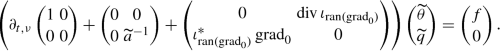
We now come to the exponential stability of the heat equation. First, we need to formulate both the heat flux balance and Fourier’s law as a suitable evolutionary equation. For doing so, we assume that $\Omega \subseteq \mathbb {R}^{d}$ is open and contained in a slab. Then $\operatorname {ran}( \operatorname {\mathrm {grad}}_{0})$ is closed by Corollary 11.3.2. It is clear that we can write Fourier’s law as

$$\displaystyle \begin{aligned} q=-a\operatorname{\mathrm{grad}}_{0}\theta=-a\iota_{\operatorname{ran}(\operatorname{\mathrm{grad}}_{0})}\iota_{\operatorname{ran}(\operatorname{\mathrm{grad}}_{0})}^{\ast}\operatorname{\mathrm{grad}}_{0}\theta. \end{aligned}$$

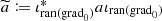
Hence, defining and , we arrive at

$$\displaystyle \begin{aligned} \widetilde{q}=-\widetilde{a}\iota_{\operatorname{ran}(\operatorname{\mathrm{grad}}_{0})}^{\ast}\operatorname{\mathrm{grad}}_{0}\theta. \end{aligned}$$

Moreover, since , we derive from the heat flux balance

and hence, assuming that $\widetilde {a}$ is invertible, we may write both equations with the unknowns $(\theta ,\widetilde {q})$ as an evolutionary equation in $L_{2,\nu }(\mathbb {R};H)$ for ν > 0, where . This yields

(11.2)

For notational convenience, we set

(11.3)

Lemma 11.3.4

Let $\Omega \subseteq \mathbb {R}^{d}$ be open and contained in a slab and C as above. Then C is densely defined, closed and boundedly invertible. Moreover

Proof

The proof is left as Exercise 11.3. □

Proposition 11.3.5

Let $\Omega \subseteq \mathbb {R}^{d}$ be open and contained in a slab, a ∈ L(L ₂( Ω)^d), and c ₁ > 0 such that

$$\displaystyle \begin{aligned} \operatorname{Re} a\geqslant c_{1}. \end{aligned}$$

Then is boundedly invertible and the solution operators associated with (11.2) are exponentially stable.

Proof

For $x\in \operatorname {ran}( \operatorname {\mathrm {grad}}_{0})$ we have

$$\displaystyle \begin{aligned} \operatorname{Re}\left\langle x ,\widetilde{a}x\right\rangle _{\operatorname{ran}(\operatorname{\mathrm{grad}}_{0})} & =\operatorname{Re}\left\langle \iota_{\operatorname{ran}(\operatorname{\mathrm{grad}}_{0})}x ,a\iota_{\operatorname{ran}(\operatorname{\mathrm{grad}}_{0})}x\right\rangle _{L_2(\Omega)^{d}}\\ & \geqslant c_{1}\left\Vert \iota_{\operatorname{ran}(\operatorname{\mathrm{grad}}_{0})}x \right\Vert {}_{L_2(\Omega)^{d}}^{2} =c_{1}\left\Vert x \right\Vert {}_{\operatorname{ran}(\operatorname{\mathrm{grad}}_{0})}^{2}, \end{aligned} $$

and thus, $\widetilde {a}$ is boundedly invertible. Hence, (11.2) is an evolutionary equation of the form considered in Theorem 11.2.1 with , for $z\in \mathbb {C}$ and C given by (11.3). Since $\operatorname {Re}\widetilde {a}^{-1}\geqslant \frac {c_{1}}{\left \Vert \widetilde {a} \right \Vert ^{2}}$, Theorem 11.2.1 is applicable and we derive the exponential stability. □

The Heat Equation with Additional Delay

Again we consider the heat equation, but now we replace Fourier’s law by

$$\displaystyle \begin{aligned} q=-a_{1}\operatorname{\mathrm{grad}}_{0}\theta-a_{2}\tau_{-h}\operatorname{\mathrm{grad}}_{0}\theta \end{aligned}$$

for some operators a ₁, a ₂ ∈ L(L ₂( Ω)^d) and h > 0. As above, we assume that $\Omega \subseteq \mathbb {R}^d$ is open and contained in a slab. We may introduce and for j ∈{1, 2}. Moreover, we assume that there exists c > 0 such that

$$\displaystyle \begin{aligned} \operatorname{Re} a_{1}\geqslant c. \end{aligned}$$

By Lemma 7.3.1 there exists ν ₀ > 0 such that the operator $\widetilde {a}_{1}+\widetilde {a}_{2}\tau _{-h}$ is boundedly invertible in $L_{2,\nu }(\mathbb {R};\operatorname {ran}( \operatorname {\mathrm {grad}}_{0}))$ and its inverse is uniformly strictly positive definite for each $\nu \geqslant \nu _0$. Hence, we may write the heat equation with additional delay as an evolutionary equation of the form

$$\displaystyle \begin{aligned} \left(\partial_{t,\nu}\begin{pmatrix} 1 & 0\\ 0 & 0 \end{pmatrix}+\begin{pmatrix} 0 & 0\\ 0 & (\widetilde{a}_{1}+\widetilde{a}_{2}\tau_{-h})^{-1} \end{pmatrix}+\begin{pmatrix} 0 & -C^{\ast}\\ C & 0 \end{pmatrix}\right)\begin{pmatrix} \theta\\ \widetilde{q} \end{pmatrix}=\begin{pmatrix} f\\ 0 \end{pmatrix}{} \end{aligned} $$

(11.4)

with C given by (11.3).

Proposition 11.3.6

Let $\Omega \subseteq \mathbb {R}^{d}$ be open and contained in a slab, h > 0, a ₁, a ₂ ∈ L(L ₂( Ω)^d), and c > 0 such that

$$\displaystyle \begin{aligned} \operatorname{Re} a_{1}\geqslant c \end{aligned}$$

and $\left \Vert a_{2} \right \Vert <c$ . Then the solution operators $(S_\nu )_{\nu \geqslant \nu _0}$ associated with (11.4) are exponentially stable.

Proof

Note that $\left \Vert \widetilde {a}_2 \right \Vert \leqslant \left \Vert a_2 \right \Vert <c$. We choose

$$\displaystyle \begin{aligned} 0<\rho_{1}<\frac{1}{h}\log\frac{c}{\left\Vert \widetilde{a}_{2} \right\Vert }. \end{aligned}$$

Then we estimate for $z\in \mathbb {C}_{\operatorname {Re}>-\rho _{1}}$

$$\displaystyle \begin{aligned} \operatorname{Re}\left\langle x ,\big(\widetilde{a}_{1}+\widetilde{a}_{2}\mathrm{e}^{-zh}\big)x\right\rangle _{\operatorname{ran}(\operatorname{\mathrm{grad}}_{0})}\geqslant(c-\left\Vert \widetilde{a}_{2} \right\Vert \mathrm{e}^{\rho_{1}h})\left\Vert x \right\Vert {}_{\operatorname{ran}(\operatorname{\mathrm{grad}}_{0})}^{2}. \end{aligned}$$

By the choice of ρ ₁, we infer . Hence,

is well-defined and satisfies

$$\displaystyle \begin{aligned} \operatorname{Re} M_{1}(z)\geqslant c_{1}\quad (z\in\mathbb{C}_{\operatorname{Re}>-\rho_{1}}) \end{aligned}$$

for some c ₁ > 0 by Proposition 6.2.3. Thus, Theorem 11.2.1 is applicable and yields the exponential stability of (11.4). □

A Dual Phase Lag Model

In this last variant of heat conduction, we replace Fourier’s law by

$$\displaystyle \begin{aligned} (1+s_{q}\partial_t)q=(1+s_{\theta}\partial_t)\operatorname{\mathrm{grad}}_{0}\theta, \end{aligned}$$

where s _q, s _θ > 0 are the so-called “phases” (cf. Sect. 7.4, where a different type of dual phase lag model is studied). The latter equation can be reformulated as

$$\displaystyle \begin{aligned} (1+s_{q}\partial_{t,\nu})(1+s_{\theta}\partial_{t,\nu})^{-1}q=\operatorname{\mathrm{grad}}_{0}\theta \end{aligned}$$

for ν > 0. Assuming that $\Omega \subseteq \mathbb {R}^d$ is open and contained in a slab, and defining , the dual phase lag model may be written as

$$\displaystyle \begin{aligned} \left(\partial_{t,\nu}\begin{pmatrix} 1 & 0\\ 0 & 0 \end{pmatrix}+\begin{pmatrix} 0 & 0\\ 0 & (1+s_{q}\partial_{t,\nu})(1+s_{\theta}\partial_{t,\nu})^{-1} \end{pmatrix}+\begin{pmatrix} 0 & -C^{\ast}\\ C & 0 \end{pmatrix}\right)\begin{pmatrix} \theta\\ \widetilde{q} \end{pmatrix}=\begin{pmatrix} f\\ 0 \end{pmatrix}{} \end{aligned} $$

(11.5)

with C given by (11.3).

Proposition 11.3.7

Let $\Omega \subseteq \mathbb {R}^{d}$ be open and contained in a slab, ν ₀ > 0. Moreover, let s _θ > s _q > 0. Then the solution operators $(S_\nu )_{\nu \geqslant \nu _0}$ associated with (11.5) are exponentially stable.

Proof

Again, we note that (11.5) is of the form considered in Theorem 11.2.1 with and

Setting we compute

$$\displaystyle \begin{aligned} \operatorname{Re} M_{1}(z)=\operatorname{Re}\left(\mu+\frac{(1-\mu)}{1+s_{\theta}z}\right)=\mu+(1-\mu)\frac{1+s_{\theta}\operatorname{Re} z}{|1+s_{\theta}z|{}^{2}}\geqslant\mu\quad (z\in\mathbb{C}_{\operatorname{Re}>-s_{\theta}^{-1}}). \end{aligned}$$

Thus, Theorem 11.2.1 is applicable and hence, the claim follows. □

11.4 Exponential Stability for Hyperbolic-Type Equations

Important examples of exponentially stable equations do not fit in the class of parabolic-like equations studied in Sect. 11.2. As a motivating example we consider the damped wave equation, which can be written as a second-order equation of the form

(11.6)

where M ₀, M ₁ ∈ L(L ₂( Ω)), M ₀ is selfadjoint and $M_{0},\operatorname {Re} M_{1}\geqslant c>0$, with $\Omega \subseteq \mathbb {R}^{d}$ modelling the underlying medium. It is well-known that this equation is exponentially stable if Ω is bounded. However, if we write this equation as an evolutionary problem in the canonical way; that is, we introduce and as new unknowns, we end up with an equation of the form

(11.7)

which is not of the form discussed in Sect. 11.2. However, another formulation of (11.6) as an evolutionary equation allows to show exponential stability in a similar way as for parabolic-type equations. More precisely, we aim for a formulation, such that the second block operator matrix in (11.7) has non-vanishing diagonal entries. This leads to a damping effect for both unknowns.

We start to provide a general reformulation scheme of second-order equations as suitable evolutionary equations and afterwards discuss the exponential stability of those.

An Alternative Reformulation for Hyperbolic-Type Equations

Throughout we assume that $C\colon \operatorname {dom}(C)\subseteq H_{0}\to H_{1}$ is a densely defined closed linear operator between two Hilbert spaces H ₀ and H ₁, which is additionally assumed to be boundedly invertible. Furthermore, let $M\colon \operatorname {dom}(M)\subseteq \mathbb {C}\to L(H_{0})$ be a material law of the form

$$\displaystyle \begin{aligned} M(z)=M_{0}(z)+z^{-1}M_{1}(z)\quad (z\in\operatorname{dom}(M)), \end{aligned}$$

where $M_{0},M_{1}\colon \operatorname {dom}(M)\subseteq \mathbb {C}\to L(H)$ are material laws themselves. We consider second-order problems of the form

$$\displaystyle \begin{aligned} \left(\partial_{t,\nu}^{2}M(\partial_{t,\nu})+C^{\ast}C\right)u=f,{} \end{aligned} $$

(11.8)

for a given right-hand side $f\in L_{2,\nu }(\mathbb {R};H_{0})$ and aim for conditions on M to ensure the exponential stability in a suitable sense.

Example 11.4.1

The wave equation (11.6) on a bounded domain $\Omega \subseteq \mathbb {R}^{n}$ is indeed of the form (11.8). We set , which is boundedly invertible by Poincaré’s inequality (see Proposition 11.3.1 and Lemma 11.3.4) and

$$\displaystyle \begin{aligned} M(z)=M_{0}+z^{-1}M_{1}\quad (z\in\mathbb{C}\setminus\{0\}) \end{aligned}$$

for M ₀, M ₁ ∈ L(L ₂( Ω)).

We now introduce two new unknowns to rewrite (11.8) as an evolutionary equation. For this let d > 0 and set and Then we formally get

$$\displaystyle \begin{aligned} \partial_{t,\nu} q=-C\partial_{t,\nu}u=-C(v_{d}-du)=-Cv_{d}+dCu=-Cv_{d}-dq \end{aligned}$$

and

$$\displaystyle \begin{aligned} \partial_{t,\nu}M(\partial_{t,\nu})v_{d} & =\partial_{t,\nu}^{2}M(\partial_{t,\nu})u+d\partial_{t,\nu}M(\partial_{t,\nu})u\\ & =f-C^{\ast}Cu+d\partial_{t,\nu}M_{0}(\partial_{t,\nu})u+dM_{1}(\partial_{t,\nu})u\\ & =f+C^{\ast}q+dM_{0}(\partial_{t,\nu})(v_{d}-du)+dM_{1}(\partial_{t,\nu})u\\ & =f+C^{\ast}q+dM_{0}(\partial_{t,\nu})v_{d}-d\left(M_{1}(\partial_{t,\nu})-dM_{0}(\partial_{t,\nu})\right)C^{-1}q. \end{aligned} $$

Thus, the new unknowns, v _d and q, satisfy an evolutionary equation of the form

$$\displaystyle \begin{aligned} &\left(\partial_{t,\nu}\left(\begin{array}{cc} M(\partial_{t,\nu}) & 0\\ 0 & 1 \end{array}\right)+d\left(\begin{array}{cc} -M_{0}(\partial_{t,\nu}) & \left(M_{1}(\partial_{t,\nu})-dM_{0}(\partial_{t,\nu})\right)C^{-1}\\ 0 & 1 \end{array}\right)\right.\\ &\qquad \qquad \qquad \qquad \qquad \qquad \left.+\left(\begin{array}{cc} 0 & -C^{\ast}\\ C & 0 \end{array}\right)\right)\left(\begin{array}{c} v_{d}\\ q \end{array}\right)=\left(\begin{array}{c} f\\ 0 \end{array}\right),{} \end{aligned} $$

(11.9)

with a new material law $M_{d}\colon \operatorname {dom}(M)\subseteq \mathbb {C}\to L(H_{0}\oplus H_{1})$ given by

Remark 11.4.2

We remark that the above formal computation can be done rigorously (both forward and backwards), so that indeed (11.8) and (11.9) are equivalent problems in the sense that the solutions u and (v _d, q) are linked via

$$\displaystyle \begin{aligned} v_{d}=\partial_{t,\nu}u+du,\quad q=-Cu. \end{aligned}$$

11.5 A Criterion for Exponential Stability of Hyperbolic-Type Equations

In this section we provide sufficient conditions on the material law M in order to obtain a well-posed and exponentially stable problem (11.9) for a suitable d > 0. So, we assume the same assumptions to be in effect as in the previous section.

Remark 11.5.1

Assume that (11.9) is exponentially stable with decay rate ρ ₀ > 0; that is, $v_{d}\in L_{2,-\rho }(\mathbb {R};H_{0}),\,q\in L_{2,-\rho }(\mathbb {R};H_{1})$ if $f\in L_{2,-\rho }(\mathbb {R};H_{0})\cap L_{2,\nu }(\mathbb {R};H_{0})$ for all $\rho \in \left [0,\rho _{0}\right )$ and ν > 0 large enough. Then $u,\partial _{t,\nu }u\in L_{2,-\rho }(\mathbb {R};H_{0})$ as well. Indeed, since

$$\displaystyle \begin{aligned} u=-C^{-1}q\in L_{2,-\rho}(\mathbb{R};H_{0}), \end{aligned}$$

we derive

$$\displaystyle \begin{aligned} \partial_{t,\nu}u=v_d-du\in L_{2,-\rho}(\mathbb{R};H_{0}). \end{aligned}$$

Employing Exercise 11.1, we even infer $u\in \operatorname {dom}(\partial _{t,-\rho })$ and hence, $u\in C_{-\rho }(\mathbb {R};H_{0})$ by Sobolev’s embedding theorem (see Theorem 4.1.2). Thus, we also obtain the exponential stability of (11.8) in this case.

In order to prove the exponential stability of (11.9), we have to show how a positive definiteness assumption on M allows for positive definiteness of M _d for some d > 0. We start with the following observation.

Lemma 11.5.2

Let $z\in \operatorname {dom}(M)$ , c > 0. Assume

$$\displaystyle \begin{aligned} \operatorname{Re}\left\langle u ,zM(z)u\right\rangle _{H_{0}}\geqslant c\left\Vert u \right\Vert {}_{H_{0}}^{2}\quad (u\in H_{0}). \end{aligned}$$

Then for d > 0 and (v, q) ∈ H ₀ ⊕ H ₁ it follows that

$$\displaystyle \begin{aligned} \operatorname{Re}\left\langle (v,q) ,zM_{d}(z)(v,q)\right\rangle _{H_{0}\oplus H_{1}}\geqslant\min\left\{ c-dK(d),\frac{3}{4}d+\operatorname{Re} z\right\} \left\Vert (v,q) \right\Vert {}_{H_{0}\oplus H_{1}}^{2}, \end{aligned}$$

where and for j ∈{0, 1}.

Proof

Let v ∈ H ₀ and q ∈ H ₁. Then we estimate

$$\displaystyle \begin{aligned} & \operatorname{Re}\left\langle (v,q) ,zM_{d}(z)(v,q)\right\rangle _{H_{0}\oplus H_{1}}\\ & =\operatorname{Re}\left\langle v ,zM(z)v-dM_{0}(z)v+d(M_{1}(z)-dM_{0}(z))C^{-1}q\right\rangle _{H_{0}}+\operatorname{Re}\left\langle q ,zq+dq\right\rangle _{H_{1}}\\ & \geqslant\left(c-dm_0\right)\left\Vert v \right\Vert {}_{H_{0}}^{2}-d\left(m_1+dm_0\right)\left\Vert C^{-1} \right\Vert \left\Vert q \right\Vert {}_{H_{1}}\left\Vert v \right\Vert {}_{H_{0}}+\left(\operatorname{Re} z+d\right)\left\Vert q \right\Vert {}_{H_{1}}^{2}\\ & \geqslant\left(c-dm_0-\frac{1}{4\varepsilon}d^{2}\left(m_1+dm_0\right)^{2}\left\Vert C^{-1} \right\Vert ^{2}\right)\left\Vert v \right\Vert {}_{H_{0}}^{2}+\left(\operatorname{Re} z+d-\varepsilon\right)\left\Vert q \right\Vert {}_{H_{1}}^{2}, \end{aligned} $$

for each ε > 0, where we have used the Peter–Paul inequality. Choosing $\varepsilon =\frac {d}{4}$, we obtain the assertion. □

This estimate allows us to derive the positive definiteness of M _d for a suitable choice of d > 0.

Proposition 11.5.3

Let c > 0 and assume that

$$\displaystyle \begin{aligned} \operatorname{Re}\left\langle u ,zM(z)u\right\rangle _{H_{0}}\geqslant c\left\Vert u \right\Vert {}_{H_{0}}^{2}\quad (u\in H_{0},\, z\in \operatorname{dom}(M)). \end{aligned}$$

Then there exist $\widetilde {c},d,\rho _{0}>0$ such that

$$\displaystyle \begin{aligned} \operatorname{Re}\left\langle (v,q) ,zM_{d}(z)(v,q)\right\rangle _{H_{0}\oplus H_{1}}\geqslant\widetilde{c}\left\Vert (v,q) \right\Vert {}_{H_{0}\oplus H_{1}}^{2} \end{aligned}$$

for all $z\in \operatorname {dom}(M)\cap \mathbb {C}_{\operatorname {Re}>-\rho _{0}}$ and (v, q) ∈ H ₀ ⊕ H ₁.

Proof

We note that dK(d) → 0 as d → 0, where K(d) is given as in Lemma 11.5.2. Hence, we find d > 0 such that dK(d) < c. Choosing $\rho _{0}<\frac {3}{4}d$ and using Lemma 11.5.2, we estimate for each $z\in \operatorname {dom}(M)\cap \mathbb {C}_{\operatorname {Re}>-\rho _{0}}$ and (v, q) ∈ H ₀ ⊕ H ₁

$$\displaystyle \begin{aligned} \operatorname{Re}\left\langle (v,q) ,zM_{d}(z)(v,q)\right\rangle _{H_{0}\oplus H_{1}} & \geqslant\widetilde{c} \left\Vert (v,q) \right\Vert {}_{H_{0}\oplus H_{1}}^{2}, \end{aligned} $$

where showing the assertion. □

We are now in the position to state the main result for exponential stability of hyperbolic-type equations.

Theorem 11.5.4

Let $C\colon \operatorname {dom}(C)\subseteq H_{0}\to H_{1}$ be a densely defined closed linear and boundedly invertible operator between two Hilbert spaces H ₀ and H ₁ . Furthermore, let $M\colon \operatorname {dom}(M)\subseteq \mathbb {C}\to L(H_{0})$ be a material law of the form

$$\displaystyle \begin{aligned} M(z)=M_{0}(z)+z^{-1}M_{1}(z)\quad (z\in\operatorname{dom}(M)), \end{aligned}$$

where $M_{0},M_{1}\colon \operatorname {dom}(M)\subseteq \mathbb {C}\to L(H)$ are bounded analytic functions. Assume that there exist c, ν ₀ > 0 such that $\mathbb {C}_{\operatorname {Re}>-\nu _{0}}\setminus \operatorname {dom}(M)$ is discrete and

$$\displaystyle \begin{aligned} \operatorname{Re}\left\langle u ,zM(z)u\right\rangle _{H_{0}}\geqslant c\left\Vert u \right\Vert {}_{H_{0}}^{2} \end{aligned}$$

for each $u\in H_{0},z\in \operatorname {dom}(M)$ . Then there exists some d > 0 such that problem (11.9) is well-posed and exponentially stable.

Proof

We first note that by Proposition 11.5.3 there exist $\rho _{0},d,\widetilde {c}>0$ such that

$$\displaystyle \begin{aligned} \operatorname{Re}\left\langle (v,q) ,zM_{d}(z)(v,q)\right\rangle _{H_{0}\oplus H_{1}}\geqslant\widetilde{c}\left\Vert (v,q) \right\Vert {}_{H_{0}\oplus H_{1}}^{2} \end{aligned}$$

for all $z\in \operatorname {dom}(M)\cap \mathbb {C}_{\operatorname {Re}>-\rho _{0}}$ and (v, q) ∈ H ₀ ⊕ H ₁. Since M is a material law, so is M _d and thus, well-posedness of (11.9) follows from Picard’s theorem (see Theorem 6.2.1). Since

$$\displaystyle \begin{aligned} \left(\begin{array}{cc} 0 & -C^{\ast}\\ C & 0 \end{array}\right) \end{aligned}$$

is skew-selfadjoint, the above estimate yields that $zM_{d}(z)+\left (\begin {array}{cc} 0 & -C^{\ast }\\ C & 0 \end {array}\right )$is boundedly invertible for each $z\in \operatorname {dom}(M)\cap \mathbb {C}_{\operatorname {Re}>-\rho _{0}}$ with

$$\displaystyle \begin{aligned} \sup_{z\in\operatorname{dom}(M)\cap\mathbb{C}_{\operatorname{Re}>-\rho_{0}}}\|T_d(z)\|\leqslant\frac{1}{\widetilde{c}}, \end{aligned}$$

where

Setting , we infer that T _d is defined on the whole $\mathbb {C}_{\operatorname {Re}>-\mu }$ despite a discrete set. Since T _d is holomorphic and bounded, Riemann’s theorem on removable singularities implies that T _d can be extended to a holomorphic and bounded function on $\mathbb {C}_{\operatorname {Re}>-\mu }$. We denote this extension again by T _d. In particular, T _d is a material law with $s_{b}(T_d)\leqslant -\mu$. Let now $\rho \in \left [0,\mu \right )$ and $(f,g)\in L_{2,\nu }(\mathbb {R};H_{0}\oplus H_{1})\cap L_{2,-\rho }(\mathbb {R};H_{0}\oplus H_{1})$, where ν > 0 is large enough to ensure well-posedness. By Theorem 5.3.6 we derive

$$\displaystyle \begin{aligned} T_d(\partial_{t,\nu})(f,g)=T_d(\partial_{t,-\rho})(f,g)\in L_{2,-\rho}(\mathbb{R};H_{0}\oplus H_{1}) \end{aligned}$$

and since T _d(∂ _t,ν)(f, g) is nothing but the solution of (11.9) with the right-hand side replaced by (f, g), exponential stability follows. □

Definition

We call the equation

$$\displaystyle \begin{aligned} \left(\partial_{t,\nu}^{2}M(\partial_{t,\nu})+C^{\ast}C\right)u=f \end{aligned}$$

exponentially stable if there exists some d > 0 such that the equation

$$\displaystyle \begin{aligned} \left(\partial_{t,\nu}M_{d}(\partial_{t,\nu})+\left(\begin{array}{cc} 0 & -C^{\ast}\\ C & 0 \end{array}\right)\right)v=g \end{aligned}$$

is exponentially stable.

11.6 Examples of Exponentially Stable Hyperbolic Problems

We will illustrate our findings by providing two concrete examples. Firstly, we discuss the damped wave equation in an abstract form and, secondly, we consider the dual phase lag model, as it was introduced in Sect. 7.4.

The Damped Wave Equation

We start by formulating an immediate corollary of our main stability theorem.

Corollary 11.6.1

Let $C\colon \operatorname {dom}(C)\subseteq H_{0}\to H_{1}$ be a densely defined closed linear and boundedly invertible operator between two Hilbert spaces H ₀ and H ₁ and let M ₀, M ₁ ∈ L(H ₀) such that M ₀ is selfadjoint and M ₀⩾0, $\operatorname {Re} M_{1}\geqslant c>0$ . Then the second order problem

$$\displaystyle \begin{aligned} \left(\partial_{t,\nu}^{2}M_{0}+\partial_{t,\nu}M_{1}+C^{\ast}C\right)u=f \end{aligned}$$

is exponentially stable.

Proof

We have to prove that the material law

satisfies the assumptions of Theorem 11.5.4. For $\operatorname {Re} z\geqslant 0$ we have

$$\displaystyle \begin{aligned} \operatorname{Re}\left\langle u ,zM(z)u\right\rangle _{H_{0}}\geqslant c\left\Vert u \right\Vert {}_{H_{0}}^{2}\quad (u\in H_{0}), \end{aligned}$$

since $\operatorname {Re} zM_{0}\geqslant 0$. Moreover, for $\operatorname {Re} z\in \left [-\rho _{0},0\right ]$ with $\rho _{0}<\frac {c}{\|M_{0}\|}$ (we set ) we have that

$$\displaystyle \begin{aligned} \operatorname{Re}\left\langle u ,zM(z)u\right\rangle _{H_{0}}\geqslant\left(-\rho_{0}\|M_{0}\|+c\right)\left\Vert u \right\Vert {}_{H_{0}}^{2}\quad (u\in H_{0}). \end{aligned}$$

Since $\mathbb {C}_{\operatorname {Re}>-\rho _{0}}\setminus \operatorname {dom}(M)=\{0\}$, we can apply Theorem 11.5.4. □

We now come to a concrete realisation of the operator C. Let $\Omega \subseteq \mathbb {R}^{d}$ be open and contained in a slab. According to Corollary 11.3.2 the space $\operatorname {ran}( \operatorname {\mathrm {grad}}_{0})$ is closed and by Lemma 11.3.4 the operator

is densely defined, closed and boundedly invertible, and its adjoint is given by

Thus, we have that

Let now M ₀, M ₁ ∈ L(L ₂( Ω)) with M ₀ selfadjoint and M ₀⩾0, $\operatorname {Re} M_{1}\geqslant c>0$. By Corollary 11.6.1 the equation

(11.10)

is exponentially stable.

Remark 11.6.2

We emphasise that this result yields the classical exponential stability for the damped wave equation; i.e., the situation where M ₀ = 1. However, Corollary 11.6.1 is also applicable in the situation where for some Ω₀ ⊆ Ω and $\operatorname {Re} M_{1}\geqslant c$. In this case, Eq. (11.10) is a coupled system of the damped wave equation inside Ω₀ and of the heat equation outside Ω₀.

Dual Phase Lag Heat Conduction

We recall the setting of Sect. 7.4, where we have discussed the equations of dual phase lag heat conduction on an open and bounded subset $\Omega \subseteq \mathbb {R}^{d}$ within the framework of evolutionary equations. The equations under consideration consist of the heat flux balance

and a modified Fourier’s law

$$\displaystyle \begin{aligned} (1+s_{q}\partial_{t,\nu}+\frac{1}{2}s_{q}^{2}\partial_{t,\nu}^{2})q=-(1+s_{\theta}\partial_{t,\nu})\operatorname{\mathrm{grad}}\theta,{} \end{aligned} $$

(11.11)

where $s_{q}\in \mathbb {R},s_{\theta }>0$ are given. Note that (1 + s _θ ∂ _t,ν) is boundedly invertible for $\nu >-\frac {1}{s_{\theta }}$ and hence, (11.11) yields

$$\displaystyle \begin{aligned} -\operatorname{\mathrm{grad}}\theta=\partial_{t,\nu}(\partial_{t,\nu}^{-1}+s_{q}+\frac{1}{2}s_{q}^{2}\partial_{t,\nu})(1+s_{\theta}\partial_{t,\nu})^{-1}q. \end{aligned}$$

Applying the operator $\partial _{t,\nu }(\partial _{t,\nu }^{-1}+s_{q}+\frac {1}{2}s_{q}^{2}\partial _{t,\nu })(1+s_{\theta }\partial _{t,\nu })^{-1}$ to the heat flux balance equation (and assuming that $Q\in \operatorname {dom}(\partial _{t,\nu })$) we obtain the following second order problem

(11.12)

for a suitable source term $\widetilde {Q}$. Assuming Dirichlet boundary conditions for θ, the equation takes the form

$$\displaystyle \begin{aligned} \left(\partial_{t,\nu}^{2}M(\partial_{t,\nu})+C^{\ast}C\right)\theta=\widetilde{Q}, \end{aligned}$$

with and

$$\displaystyle \begin{aligned} M(z)=\frac{z^{-1}+s_{q}+\frac{1}{2}s_{q}^{2}z}{1+s_{\theta}z}\quad \left(z\in\mathbb{C}\setminus\left\{0,-\frac{1}{s_{\theta}}\right\}\right). \end{aligned}$$

Note that

$$\displaystyle \begin{aligned} M(z)=\frac{s_{q}+\frac{1}{2}s_{q}^{2}z}{1+s_{\theta}z}+z^{-1}\frac{1}{1+s_{\theta}z} \end{aligned}$$

and hence, M is indeed of the form considered in Sect. 11.5 with

$$\displaystyle \begin{aligned} M_{0}(z) & =\frac{s_{q}+\frac{1}{2}s_{q}^{2}z}{1+s_{\theta}z},\quad M_{1}(z) =\frac{1}{1+s_{\theta}z}, \end{aligned} $$

which are both bounded if we restrict the domain of M to a right half-plane $\mathbb {C}_{\operatorname {Re}>-\frac {1}{s_{\theta }}+\varepsilon }$ for some ε > 0.

Proposition 11.6.3

If $0<\frac {s_{q}}{s_{\theta }}<2$ then the dual phase lag model (11.12) is exponentially stable.

Proof

We apply Theorem 11.5.4. For this we need to show that there exists c > 0 such that

$$\displaystyle \begin{aligned} \operatorname{Re}\left\langle u ,zM(z)u\right\rangle _{L_2(\Omega)}\geqslant c\left\Vert u \right\Vert {}_{L_2(\Omega)}^{2} \end{aligned}$$

for each u ∈ L ₂( Ω) and $z\in \mathbb {C}_{\operatorname {Re}>-\nu _{0}}\cap \operatorname {dom}(M)$ for some $0<\nu _{0}<\frac {1}{s_{\theta }}$. Indeed, this is sufficient for exponential stability, since $\mathbb {C}_{\operatorname {Re}>-\nu _{0}}\setminus \operatorname {dom}(M)=\{0\}$ is discrete and $C=\iota _{\operatorname {ran}( \operatorname {\mathrm {grad}}_{0})}^{\ast } \operatorname {\mathrm {grad}}_{0}$ is boundedly invertible. Similar to the proof of Lemma 7.4.3 we set and obtain

$$\displaystyle \begin{aligned} zM(z)=\frac{1}{2}s_{q}z\sigma+\sigma\left(1-\frac{1}{2}\sigma\right)+\frac{1-\sigma(1-\frac{1}{2}\sigma)}{1+s_{\theta}z} \end{aligned}$$

for each $z\in \operatorname {dom}(M)$. Since 0 < σ < 2 we obtain $0<\sigma \left (1-\frac {1}{2}\sigma \right )\leqslant \frac {1}{2}$ and hence,

$$\displaystyle \begin{aligned} \operatorname{Re} zM(z) & =\frac{1}{2}s_{q}\operatorname{Re} z\sigma+\sigma\left(1-\frac{1}{2}\sigma\right)+\frac{\left(1-\sigma(1-\frac{1}{2}\sigma)\right)(1+s_{\theta}\operatorname{Re} z)}{\left|1+s_{\theta}z\right|{}^{2}}\\ & \geqslant-\frac{1}{2}s_{q}\nu_{0}\sigma+\sigma(1-\frac{1}{2}\sigma)=: c_{\nu_{0}} \end{aligned} $$

for each $z\in \mathbb {C}_{\operatorname {Re}>-\nu _{0}}\cap \operatorname {dom}(M)$ with $0<\nu _{0}<\frac {1}{s_{\theta }}.$ Choosing now $0<\nu _{0}<\min \{\frac {1}{s_{\theta }},\frac {2-\sigma }{s_{q}}\}$, we obtain $c_{\nu _{0}}>0$ and thus, Theorem 11.5.4 is applicable which yields the assertion. □

11.7 Comments

The results of this chapter are based on the results obtained in [116, Section 2]. There, Laplace transform techniques are used to characterise the exponential stability of evolutionary equations in a slightly more general setting. In particular, further criteria for exponential stability of parabolic- and hyperbolic-type equations are given, which also allow for the treatment of integro-differential equations.

In general whether or not a given partial differential equation is (exponentially) stable is both an important and classical question in the area of equations depending on time. The understanding of this question for instance contributes to the study of equilibria of non-linear equations. In the linear case, in particular in the framework of C ₀-semigroups, stability has been studied intensively resulting in an abundance of criteria. Due to strong continuity of the semigroup and, thus, of the considered solutions (exponential) stability is defined via pointwise estimates. As an example criterion we mention Datko’s theorem [29] (see also [6, Theorem 5.1.2]), which states that a C ₀-semigroup is exponentially stable if and only if the solution operator associated with the equation

$$\displaystyle \begin{aligned} \left(\partial_{t,\nu}+A\right)U=F \end{aligned}$$

leaves $L_{p}(\mathbb {R}_{\geqslant 0};H)$ invariant for some (or equivalently all) $p\in \left [1,\infty \right )$. As it turns out, the latter is equivalent to the invariance of $L_{2,-\rho }(\mathbb {R};H)$ for some ρ > 0 and thus, our notion of exponential stability coincides with the usual one used in the theory of C ₀-semigroups. Another important theorem on the exponential stability of C ₀-semigroups on Hilbert spaces is the Theorem of Gearhart–Prüß [96] (see also [38, Chapter 5, Theorem 1.11]), where the exponential stability of a C ₀-semigroup is characterised in terms of the resolvent of its generator.

The wave equation without damping is not exponentially stable. In fact one can even show that energy is preserved during the evolution. Hence, it is a natural question whether it is possible to introduce suitable ‘dampers’ (i.e., lower order coefficients) leading to an exponentially stable equation. The criterion in Corollary 11.6.1 shows that if the damper M ₁ is ‘global’ in the sense that it is induced by a multiplication operator a(m) for a strictly positive function a, the resulting damped wave equation is exponentially stable.

A less general, more detailed analysis of the actual wave equation shows that it is possible to obtain an exponentially stable damped wave equation if the damper is only local or introduced via boundary conditions. Indeed, in [9] the authors proved exponential stability of the damped equation if the damping area satisfies the geometric optics condition. This is, for instance, the case if [a > 0] contains a neighbourhood of the boundary ∂ Ω.

Besides exponential stability, which is the only type of stability studied so far within the current framework of evolutionary equations, different kinds of asymptotic behaviours were addressed and characterised for C ₀-semigroups. We just mention the celebrated Arendt–Batty–Lyubich–Vu theorem [4, 61] on strong stability of C ₀-semigroups or the Theorem of Borichev–Tomilov [15] on the polynomial stability of C ₀-semigroups on Hilbert spaces.

Exercises

Exercise 11.1

Let H be a Hilbert space, $\nu ,\rho \in \mathbb {R}$ and $u\in L_{1,\mathrm {loc}}(\mathbb {R};H)$. Prove the following statements:

• (a) If $u\in \operatorname {dom}(\partial _{t,\nu })\cap \operatorname {dom}(\partial _{t,\rho })$ then ∂ _t,ν u = ∂ _t,ρ u.

• (b) If $u\in \operatorname {dom}(\partial _{t,\nu })$ such that $u,\partial _{t,\nu }u\in L_{2,\rho }(\mathbb {R};H)$ then $u\in \operatorname {dom}(\partial _{t,\rho })$.

Exercise 11.2

Prove Lemma 11.3.3.

Exercise 11.3

Let H ₀, H ₁ be Hilbert spaces and $A\colon \operatorname {dom}(A)\subseteq H_{0}\to H_{1}$ a densely defined closed linear operator. Moreover, we assume that A has closed range. Show that the adjoint of the operator $\iota _{\operatorname {ran}(A)}^{\ast }A\colon \operatorname {dom}(A)\subseteq H_{0}\to \operatorname {ran}(A)$ is given by $A^{\ast }\iota _{\operatorname {ran}(A)}$. If additionally A is one-to-one, show that $\iota _{\operatorname {ran}(A)}^\ast A$ is boundedly invertible.

Exercise 11.4

Let $\Omega \subseteq \mathbb {R}^{d}$ be open and contained in a slab. We consider the heat conduction with a memory term given by the equations

(11.13)

where $k\in L_{1,-\rho _{1}}(\mathbb {R}_{\geqslant 0};\mathbb {R})$ for some ρ ₁ > 0 with

$$\displaystyle \begin{aligned} \int_{0}^{\infty}\left\vert k(t) \right\vert \,\mathrm{d} t<1. \end{aligned}$$

Write (11.13) as a suitable evolutionary equation and prove that this equation is exponentially stable.

Exercise 11.5

Let $A\in \mathbb {C}^{n\times n}$ for some $n\in \mathbb {N}$ and consider the evolutionary equation

$$\displaystyle \begin{aligned} (\partial_{t,\nu}+A)U=F. \end{aligned}$$

Prove that the solution operators associated with this problem are exponentially stable if and only if A has only eigenvalues with strictly positive real part.

Exercise 11.6

Let $\Omega \subseteq \mathbb {R}^{d}$ be open.

• (a) Let $\varphi \in C_{\mathrm {c}}^\infty (\Omega )^{d}$. Prove Korn’s inequality

  $$\displaystyle \begin{aligned} \left\Vert \operatorname{\mathrm{Grad}}\varphi \right\Vert {}_{L_2(\Omega)_{\mathrm{sym}}^{d\times d}}^{2}\geqslant\frac{1}{2}\sum_{j=1}^{d}\left\Vert \operatorname{\mathrm{grad}}\varphi_{j} \right\Vert {}_{L_2(\Omega)^{d}}^{2}. \end{aligned}$$

• (b) Use Korn’s inequality to prove that for u ∈ L ₂( Ω)^d we have

  $$\displaystyle \begin{aligned} u\in\operatorname{dom}(\operatorname{\mathrm{Grad}}_{0})\quad \Longleftrightarrow\quad \forall j\in\{1,\ldots,d\}:\:u_{j}\in\operatorname{dom}(\operatorname{\mathrm{grad}}_{0}). \end{aligned}$$

  Moreover, show that in either case

  $$\displaystyle \begin{aligned} \frac{1}{2}\sum_{j=1}^{d}\left\Vert \operatorname{\mathrm{grad}}_{0}u_{j} \right\Vert {}_{L_2(\Omega)^{d}}^{2}\leqslant\left\Vert \operatorname{\mathrm{Grad}}_{0}u \right\Vert {}_{L_2(\Omega)_{\mathrm{sym}}^{d\times d}}^{2}\leqslant\sum_{j=1}^{d}\left\Vert \operatorname{\mathrm{grad}}_{0}u_{j} \right\Vert {}_{L_2(\Omega)^{d}}^{2}. \end{aligned}$$

• (c) Let now Ω be contained in a slab. Prove that $\operatorname {\mathrm {Grad}}_{0}$ is one-to-one and has closed range.

Exercise 11.7

Let $\Omega \subseteq \mathbb {R}^d$ be open and a ∈ L(L ₂( Ω)^d) with $\operatorname {Re} a\geqslant c>0$.

• (a) Let ν > 0 and $f\in L_{2,\nu }(\mathbb {R};L_2(\Omega ))$. Moreover, assume that Ω is contained in a slab and define . Let $\theta \in L_{2,\nu }(\mathbb {R};L_2(\Omega ))$, $q\in L_{2,\nu }(\mathbb {R};L_2(\Omega )^d)$ satisfy

  

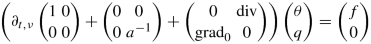
  and $\widetilde {\theta }\in L_{2,\nu }(\mathbb {R};L_2(\Omega ))$, $\widetilde {q}\in L_{2,\nu }(\mathbb {R};\operatorname {ran}( \operatorname {\mathrm {grad}}_0))$ satisfy

  

  Show that $(\theta ,\iota _{\operatorname {ran}( \operatorname {\mathrm {grad}}_0)}^\ast q)=(\widetilde {\theta },\widetilde {q})$.

• (b) Let Ω be bounded and consider the evolutionary equation

  

  Show that the associated solution operators are not exponentially stable.

References

W. Arendt, C.J.K. Batty, Tauberian theorems and stability of one-parameter semigroups. Trans. Am. Math. Soc. 306(2), 837–852 (1988)
W. Arendt et al., Vector-Valued Laplace Transforms and Cauchy Problems, 2nd edn. (Birkhäuser, Basel, 2011)
C. Bardos, G. Lebeau, J. Rauch, Sharp sufficient conditions for the observation, control, and stabilization of waves from the boundary. SIAM J. Control Optim. 30(5), 1024–1065 (1992)
A. Borichev, Y. Tomilov, Optimal polynomial decay of functions and operator semigroups. Math. Ann. 347(2), 455–478 (2010)
R. Datko, Uniform asymptotic stability of evolutionary processes in a Banach space. SIAM J. Math. Anal. 3, 428–445 (1972)
K.-J. Engel, R. Nagel, One-Parameter Semigroups for Linear Evolution Equations, vol. 194. Graduate Texts in Mathematics. With contributions by S. Brendle, M. Campiti, T. Hahn, G. Metafune, G. Nickel, D. Pallara, C. Perazzoli, A. Rhandi, S. Romanelli, R. Schnaubelt (Springer, New York, 2000)
Y.I. Lyubich, Q.P. Vũ, Asymptotic stability of linear differential equations in Banach spaces. Studia Math. 88(1), 37–42 (1988)
J. Prüss, On the spectrum of C 0-semigroups. Trans. Am. Math. Soc. 284(2), 847–857 (1984)
S. Trostorff, Exponential Stability and Initial Value Problems for Evolutionary Equations. Habilitation Thesis. TU Dresden, 2018
Author information
Authors and Affiliations
Rights and permissions
Open Access This chapter is licensed under the terms of the Creative Commons Attribution 4.0 International License (http://creativecommons.org/licenses/by/4.0/), which permits use, sharing, adaptation, distribution and reproduction in any medium or format, as long as you give appropriate credit to the original author(s) and the source, provide a link to the Creative Commons license and indicate if changes were made.
The images or other third party material in this chapter are included in the chapter's Creative Commons license, unless indicated otherwise in a credit line to the material. If material is not included in the chapter's Creative Commons license and your intended use is not permitted by statutory regulation or exceeds the permitted use, you will need to obtain permission directly from the copyright holder.
Copyright information
© 2022 The Author(s)
About this chapter
Cite this chapter
Seifert, C., Trostorff, S., Waurick, M. (2022). Exponential Stability of Evolutionary Equations. In: Evolutionary Equations. Operator Theory: Advances and Applications, vol 287. Birkhäuser, Cham. https://doi.org/10.1007/978-3-030-89397-2_11
Download citation
DOI: https://doi.org/10.1007/978-3-030-89397-2_11
Published:
Publisher Name: Birkhäuser, Cham
Print ISBN: 978-3-030-89396-5
Online ISBN: 978-3-030-89397-2
eBook Packages: Mathematics and StatisticsMathematics and Statistics (R0)