
Abstract
In this final chapter, we consider quotients of the upper half-plane by quaternionic unit groups as generalizations of such quotients from the matrix group (Chapter 40), realizing them as moduli spaces for abelian surfaces with quaternionic multiplication. This chapter can be seen as a culminating application of all of the parts of this book, and for that reason, is necessarily more advanced. Concepts are reviewed in the attempt to be self-contained, but additional background in algebraic and arithmetic geometry is suggested.
You have full access to this open access chapter, Download chapter PDF
In this final chapter, we consider quotients of the upper half-plane by quaternionic unit groups as generalizations of such quotients from the matrix group (Chapter 40), realizing them as moduli spaces for abelian surfaces with quaternionic multiplication. This chapter can be seen as a culminating application of all of the parts of this book, and for that reason, is necessarily more advanced. Concepts are reviewed in the attempt to be self-contained, but additional background in algebraic and arithmetic geometry is suggested.
1 \(\triangleright \) QM abelian surfaces
Recall (40.1.1) that the curve \({{\,\mathrm{SL}\,}}_2(\mathbb Z ) \backslash \mathbf{\textsf {H} }^2\) parametrizes complex elliptic curves up to isomorphism: to \(\tau \in \mathbf{\textsf {H} }^2\), we associate the lattice \(\Lambda _\tau :=\mathbb Z + \mathbb Z \tau \) and the elliptic curve \(E_\tau :=\mathbb C /\Lambda _\tau \), and the association
is bijective. Moreover, we have a biholomorphic map \(j:{{\,\mathrm{SL}\,}}_2(\mathbb Z ) \backslash \mathbf{\textsf {H} }^2\rightarrow \mathbb C \), which is to say, two complex elliptic curves are isomorphic if and only if they have the same j-invariant. We compactify to \(X :={{\,\mathrm{SL}\,}}_2(\mathbb Z ) \backslash \mathbf{\textsf {H} }^{2*}\) by including the cusp at \(\infty \).
As in section 38.1, we are led to seek a generalization of (43.1.1), replacing \(B={{\,\mathrm{M}\,}}_2(\mathbb Q )\) with a quaternion algebra. To this end, let B be an indefinite quaternion algebra over \(\mathbb Q \) of discriminant D, let \(\mathcal {O}\subset B\) be a maximal order, and let
be an embedding (explicitly, we may take (38.1.1)). The order \(\mathcal {O}\) is unique up to conjugation in B (by strong approximation) and similarly the embedding \(\iota _\infty \) is unique up to conjugation in \({{\,\mathrm{M}\,}}_2(\mathbb R )\), so these choices are harmless. Let
The quotient \(\Gamma ^1(\mathcal {O}) \backslash \mathbf{\textsf {H} }^2\) is compact when \(B \not \simeq {{\,\mathrm{M}\,}}_2(\mathbb Q )\); for uniformity, we define
where \(\mathbf{\textsf {H} }^{2(*)}=\mathbf{\textsf {H} }^{2*},\mathbf{\textsf {H} }^2\) according as \(D=1\) or \(D>1\). Then \(X^1\) is a good (compact) complex 1-orbifold.
We may then ask: what does \(X^1\) parametrize? The answer is, roughly: \(X^1\) parametrizes complex abelian surfaces with endomorphisms by \(\mathcal {O}\). The correspondence itself is as pleasingly simple as for elliptic curves (43.1.1). To a point \(\tau \in \mathbf{\textsf {H} }^2\), we associate
Then \(A_\tau \) is a complex torus of dimension 2 and \(\iota _\tau \) is an injective ring homomorphism, realizing endomorphisms of \(A_\tau \) by \(\mathcal {O}\).
However, there are a number of technical points required to make this completely precise. We quickly survey the theory of complex abelian varieties in section 43.4. One basic fact of life is that not every complex torus has enough meromorphic functions to give it the structure of a complex abelian variety embedded in projective space. One needs a polarization given by a Riemann form, and the simplest polarizations are the principal polarizations. (One can think of this rigidification as the difference between a genus 1 curve and an elliptic curve, where the genus 1 curve is equipped with a point.) A principal polarization defines positive involution on the endomorphism ring, called the Rosati involution.
This rigidification is matched on the quaternion order: a principal polarization on \(\mathcal {O}\) is an element \(\mu \in \mathcal {O}\) such that \(\mu ^2+D=0\). Every (maximal) order has a principal polarization, and the involution \(\alpha \mapsto \alpha ^*=\mu ^{-1}\overline{\alpha } \mu \) is a positive involution on \(\mathcal {O}\). A quaternionic multiplication (QM) structure by \((\mathcal {O},\mu )\) on a principally polarized complex abelian surface A is an injective ring homomorphism \(\mathcal {O}\hookrightarrow {{\,\mathrm{End}\,}}(A)\) that respects the positive involutions on B and \({{\,\mathrm{End}\,}}(A)_\mathbb Q \).
The happy fact is that \(A_\tau \) as defined in (43.1.2) has via \(\mu \) a principal polarization and thereby QM by \((\mathcal {O},\mu )\). In other words, the choice of the QM structure determines a canonical principal polarization: but it gives a finite amount of additional information, as there will in general be more than one QM structure on a principally polarized abelian surface. In many cases, these structures can be understood in terms of the Atkin–Lehner group
acting by automorphisms of \(X^1\).
In any event, the main result of this chapter (Main Theorem 43.6.14) is that this association is bijective.
Main Theorem 43.1.4
The map

is a bijection.
This main theorem generalizes (43.1.1): indeed, we may take \(B={{\,\mathrm{M}\,}}_2(\mathbb Q ) \supset \mathcal {O}= {{\,\mathrm{M}\,}}_2(\mathbb Z )\) and \(\mu =\begin{pmatrix} 0 &{} 1 \\ 1 &{} 0 \end{pmatrix}\), and we find that \(A_\tau \simeq E_\tau ^2\) as principally polarized abelian surfaces.
One feature that makes this theory even more appealing is that abelian surfaces arise naturally as Jacobians of genus 2 curves via the Abel–Jacobi map: this motivates much of the theory, so we begin with it in section 43.3. In particular, there are functions called Igusa invariants analogous to the elliptic j-function that record the isomorphism class of a principally polarized abelian surface.
43.1.6
We then define modular forms as for the classical modular group. Let \(k \in 2\mathbb Z _{\ge 0}\). A map \(f:\mathbf{\textsf {H} }^2\rightarrow \mathbb C \) is weight k -invariant under \(\Gamma =\Gamma ^1(\mathcal {O})\) if
A modular form for \(\Gamma \) of weight k is a holomorphic function \(f:\mathbf{\textsf {H} }^2\rightarrow \mathbb C \) that is weight k invariant and is holomorphic at \(\infty \), if \(\Gamma ={{\,\mathrm{PSL}\,}}_2(\mathbb Z )\). Let \(M_k(\Gamma )\) be the \(\mathbb C \)-vector space of modular forms for \(\Gamma \). Then \(M_k(\Gamma )\) is a finite-dimensional \(\mathbb C \)-vector space, and by a similar contour integration as in the proof of Proposition 40.3.4, \(\dim _\mathbb C M_k(\Gamma )\) can be expressed in terms of k and the signature of \(\Gamma \). And
has the structure of a graded \(\mathbb C \)-algebra under multiplication. (When \(D>1\), there are no cusps, so vacuously all modular forms are cusp forms.)
It would not be unreasonable for us to have started the book here, with this topic at front and center. In this chapter, we will do our best to treat the complex analytic theory in as complete and self-contained a manner as possible, but this is really just the beginning of the subject, one that is rich, deep, and complicated—worthy of a book all to itself. For example, the following result is fundamental.
Theorem 43.1.9
(Shimura [Shi67, p. 58]). There exists a projective nonsingular curve \(X^1\) defined over \(\mathbb Q \) and a biholomorphic map

The curve \(X^1\) over \(\mathbb Q \) coarsely represents the functor from schemes over \(\mathbb Q \) to sets whose values are isomorphism classes of QM abelian schemes, suitably defined. Moreover, the map \(\varphi \) respects the field of definition and Galois action on certain special points called CM points on \(\Gamma ^1(\mathcal {O}) \backslash \mathbf{\textsf {H} }^2\) obtained as fixed points of elements \(\nu \in B^\times \) with \(\mathbb Q (\nu )\) an imaginary quadratic field. As a result, the curve \(X^1\) is canonical, uniquely characterized up to isomorphism, and is so called the canonical model. We give some indications of this result by example in the next section and more generally in section 43.8.
2 \(\triangleright \) QM by discriminant 6
For concreteness, before embarking on our general treatment, we consider in this section an illustrative example and one of special interest; it is well-studied and beloved by quaternionic practitioners, see Remark 43.2.21 for further reference.
Let \(B=\displaystyle {\biggl (\frac{-1,3}{\mathbb {Q}}\biggr )}\) be the quaternion algebra of discriminant 6 studied in sections 37.8–37.9. As in 37.8.12, we have a maximal order
with \(k^2-k-1=0\), and an embedding
Let \(\Gamma ^1 = \iota _\infty (\mathcal {O}^1)/\{\pm 1\} \le {{\,\mathrm{PSL}\,}}_2(\mathbb R )\) and \(X^1=\Gamma ^1 \backslash \mathbf{\textsf {H} }^2\). We computed a compact Dirichlet fundamental domain  for \(\Gamma ^1\) in 37.9.4, with
  . Further, we saw explicitly in 37.9.10 (and again by formula in Example 39.4.21) that \(\Gamma ^1\) has signature (0; 2, 2, 3, 3); that is, \(X^1\) has topological genus \(g=0\) and there are 4 cone points, two points
  with stabilizer of order 2 and two
  with order 3 stabilizer.
As in Chapter 40, to exhibit a model for \(X^1\) we seek modular forms, indeed, we now describe the full graded ring of (even weight) modular forms (43.1.8). We will use the following essential proposition.
Proposition 43.2.1
The following statements hold.
-
(a)
Let \(f:\mathbf{\textsf {H} }^2\rightarrow \mathbb C \) be a nonzero meromorphic modular form of weight k for \(\Gamma ^1\), not identically zero. Then
$$\begin{aligned} \sum _{\Gamma ^1 z \in \Gamma ^1 \backslash \mathbf{\textsf {H} }^2} \frac{1}{\#{{\,\mathrm{Stab}\,}}_{\Gamma ^1}(z)}{{\,\mathrm{ord}\,}}_z(f) = \frac{k}{6}. \end{aligned}$$ -
(b)
We have
$$\begin{aligned} \dim _\mathbb C M_k(\Gamma ^1) = {\left\{ \begin{array}{ll} 1, &{} \text { if }k=0; \\ 0, &{} \text { if }k=2; \\ 1-k + 2\lfloor k/4 \rfloor + 2 \lfloor k/3 \rfloor , &{} \text { if }k \ge 4. \end{array}\right. } \end{aligned}$$(43.2.2)
Proof See Theorem 43.9.4; for the purposes of this introduction, we provide a sketch to tide the reader over. For (a), we argue just as in Proposition 40.3.4: we integrate \(\mathrm d {\log f}=\mathrm d {f}/f\) over the boundary of the fundamental domain  and use the identification of sides provided by rotation at their fixed points (elliptic vertices), reversing the direction of the path so the contributions cancel, and we are left again to sum angles. The details are requested in Exercise 43.7. For (b), we can get upper bounds on the dimension using (a), but to provide lower bounds we need to exhibit modular forms, and these are provided by the Riemann–Roch theorem. For example, for \(k=2\), we have \(\dim _\mathbb C M_2(\Gamma ^1)=g=0\) by (40.2.11).
43.2.3
We are now in a position to prove an analogous statement to Theorem 40.3.11. Referring to Proposition (43.2.1), by part (a) we seek \(a_1,a_{2},a_{2}',a_{3},a_{3}' \in \mathbb Z _{\ge 0}\) with
By part (b), we have \(\dim _\mathbb C M_k(\Gamma ^1)=0\) for \(k<0\), and indeed, there are no solutions. For \(k=0\), there is a unique solution corresponding to the constant functions. For \(k=2\), there are no solutions, as follows. Let \(f(z) \in M_2(\Gamma ^1)\). Let \(\gamma _3\) be a generator for the stabilizer at \(z_3\). Then
by the cocycle relation, we have \(1=\jmath (\gamma _3^3;z_3)=\jmath (\gamma _3;z_3)^3\) a nontrivial cube root of unity, so \(f(z_3)=0\) and \(a_3 >0\). Similarly \(a_3'>0\), and this contradicts (43.2.4).
Arguing in the same way, we find that the unique solution for \(k=4\) is \(a_2=a_2'=0\) and \(a_3=a_3'=1\); thus \(M_4(\Gamma ^1)=\mathbb C f_4\), and \(f_4\) necessarily vanishes at \(z_2,z_2'\). Similarly, for \(k=6\) we have only \(a_3=a_3'=0\) and \(a_2=a_2'=1\), with \(M_6(\Gamma ^1)=\mathbb C g_6\).
Continuing as in 43.2.3, we collect dimensions and spanning functions as in Table 43.2.5.
43.2.6
In weights 8, 10, we have products of forms seen previously. In weight \(k=12\), we find a third function \(h_{12} \in M_{12}(\Gamma ^1)\) spanning together with \(f_4^3,g_6^2\). Continuing in this way, finally in weight \(k=24\), we find 6 functions in a 5 dimensional space, and so they must satisfy an equation \(r(f_4,g_6,h_{12}) \in \mathbb C [f_4,g_6,h_{12}]\), homogeneous of degree 24 if we give \(f_4,g_6,h_{12}\) the weights 4, 6, 12.
Proposition 43.2.7
We have
Proof The bound on the degrees of generators and relations in Theorem 43.9.6 makes this proposition immediate. It is also possible to give a proof with bare hands: see Exercise 43.9.
43.2.8
We do not have Eisenstein series available in this setting, but the notion of taking averages 40.1.19 is still quite sensible: we find what are known as Poincaré series. Recall \(\jmath (\gamma ;z)=cz+d\) for \(\gamma =\begin{pmatrix} a &{} b \\ c &{} d \end{pmatrix} \in {{\,\mathrm{SL}\,}}_2(\mathbb R )\). The square \(\jmath (\gamma ;z)^2\) is well-defined on \(\gamma \in {{\,\mathrm{PSL}\,}}_2(\mathbb R )\).
For \(k \in 2\mathbb Z _{\ge 2}\), we define the Poincaré series
Then \(P_k(z)\) is nonzero, absolutely convergent on \(\mathbf{\textsf {H} }^2\), uniformly on compact subsets, and satisfies
The convergence statement is fairly tame, because the fundamental domain  is compact: it implies that the total integral
is finite, and the Poincaré series converges (absolutely) by comparison [Kat85, §1, Proposition 1]. The equality (43.2.9) follows from the cocycle relation (40.2.5). Therefore \(P_k(z) \in S_k(\Gamma )\), and in particular we may take \(f_4=P_4\) and \(g_6=P_6\); with a bit more computation, one can also show that \(P_4^3,P_6^2,P_{12}\) are linearly independent, so that we may take \(h_{12}=P_{12}\) as well.
43.2.10
A convenient and meaningful normalization of the functions above is given by Baba–Granath [BG2008, §3.1].
First, there are exactly two (necessarily optimal) embeddings \(S=\mathbb Z [\sqrt{-6}] \hookrightarrow \mathcal {O}\) by Example 30.7.5: we have \(\#{{\,\mathrm{Cls}\,}}\mathcal {O}=1\) and \(K(\sqrt{-6})\) is ramified at \(p=2,3 \mid D=6\), so \(m(S,\mathcal {O};\mathcal {O}^\times ) = h(\mathbb Z [\sqrt{-6}])=2\). The fixed points of these two embeddings are distinct points  . Explicitly, we note that
has \(\mu ^2+6=0\), and choose its fixed point as \(z_6\).
We rescale \(g_6\) so that \(f_4^3(z_6)/g_6^2(z_6)=\sqrt{-3}\), and we choose \(h_{12}\) such that \(h_{12}(z_6)=h_{12}(z_6')=0\), and rescale so that
Corollary 43.2.13
The holomorphic map
has image the conic \(X^1:x^2+3y^2+z^2=0\), defining the canonical model over \(\mathbb Q \).
Proof This result is attributed to Ihara by Kurihara [Kur79, Theorem 1-1(1)]; it is proven by Baba–Granath [BG2008, Theorem 3.10] along the lines above.
We note that \(X^1(\mathbb R )=\emptyset \); this is a general feature, see Proposition 43.7.2.
43.2.15
The Atkin–Lehner group
has three nontrivial involutions \(w_2,w_3,w_6\) with representatives having positive reduced norm. Explicitly, we have \(w_6=\mu \) by (43.2.11) and \(w_2=1+i\) and \(w_3=w_6/w_2 = 1+i-j+k\). These involutions act on the space of modular forms as follows [BG2008, §3.1]:So for example \(f_4(w_2 z) = -f_4(z)\).

These involutions act on the canonical model \(X^1\) by \(w_2(x:y:z)=(x:-y:z)\), \(w_3(-x:y:z)\), and \(w_6(x:y:z)=(x:y:-z)\).
We choose a principal polarization (see Definition 43.6.4) on \(\mathcal {O}\) by \(\mu \) in (43.2.11). In this way, Main Theorem 43.1.4 provides that the curve \(X^1\) parametrizes abelian surfaces with QM by \((\mathcal {O},\mu )\).
43.2.16
The forgetful map \([(A_\tau ,\iota _\tau )] \mapsto [A_\tau ]\) which forgets the QM structure is the map [BG2008, Proposition 3.9]
generically 4-to-1. The map j can fruitfully be thought of as an analogue of the classical elliptic j-invariant, mindful of the above technicalities: it parametrizes principally polarized complex abelian surfaces that can be equipped with a QM structure.
The Igusa invariants 43.3.5 of \(A_j\) where \(j=j(\tau )\) are given by [BG2008, Proposition 3.6]
There exists a genus 2 curve with these Igusa invariants if and only if \(j=0,-16/27\) or the Hilbert symbol
is trivial.
Example 43.2.19
The two points with \(j=0,\infty \) are exactly those points which are not Jacobians of genus 2 curves: these correspond to points with CM by \(\mathbb Z [\sqrt{-1}]\) and \(\mathbb Z [\omega ]\), and these abelian surfaces are the squares of the corresponding CM elliptic curves (with the product polarization). Elkies [Elk98, §3] computes equations and further CM points for discriminant 6.
Example 43.2.20
The case \(j=-16/27\) corresponds to a CM point with discriminant \(D=-24\) [BG2008, §3.3]: it is the Jacobian of the curve
isomorphic to the product of the two elliptic curves with CM by \(\mathbb Z [\sqrt{-6}]\) (but not with the product polarization).
Remark 43.2.21. For further reading to connect some of the dots above, see the article by Baba–Granath [BG2008], refining the work by Hashimoto–Murabayashi [HM95, Theorem 1.3] who give an explicit family of genus 2 curves whose Jacobians have QM by \(\mathcal {O}\).
3 Genus 2 curves
We begin in the concrete setting of genus 2 curves. Let F be a perfect field with \({{\,\mathrm{char}\,}}F \ne 2\) and let \(F{}^{al }\) be an algebraic closure of F. Let X be a smooth projective curve of genus 2 over F.
43.3.1
Using Riemann–Roch in a manner analogous to the proof for elliptic curves (see e.g. Silverman [Sil2009, Proposition III.3.1(a)]), X is given by a Weierstrass equation of the form
where \(f(x) \in F[x]\) is squarefree of degree 5 or 6. It follows that X is hyperelliptic over F, with map \(x:X \rightarrow \mathbb P ^1\) of degree 2.
If \((y')^2=f'(x')\) is another Weierstrass equation for X, then it is related by a change of variables of the form
with \(ad-bc,e \in F^\times \). After such a change of variable, we may suppose without loss of generality that \(\deg f=6\).
Example 43.3.4
Let \(X{}^{al }\) be the base change of X to \(F{}^{al }\). The automorphism group \({{\,\mathrm{Aut}\,}}(X{}^{al })\) is a finite group containing the hyperelliptic involution \((x,y) \mapsto (x,-y)\). The possibilities for this group were classified by Bolza [Bol1887, p. 70]: when \({{\,\mathrm{char}\,}}F \ne 2,3,5\), the group \({{\,\mathrm{Aut}\,}}(X{}^{al })\) is isomorphic to one of the groups
of orders 2, 4, 8, 10, 12, 24, 48. A generic genus 2 curve over \(F{}^{al }\) has \({{\,\mathrm{Aut}\,}}(X{}^{al }) \simeq C_2\).
43.3.5
We now seek invariants of the curve defined in terms of a model to classify isomorphism classes. We factor
with \(a_i \in F{}^{al }\) the roots of f. We abbreviate \(a_i - a_j\) by \((i \,j)\), and we define
where each sum and product runs over the distinct expressions obtained by permuting the index set \(\{1, \dots ,6\}\); by Galois theory, we have \(I_2,I_4,I_6,I_{10} \in F\). In particular, we have
is the discriminant of the polynomial 4f. The invariants \(I_2, I_4, I_6, I_{10}\), defined by Igusa [Igu60, p. 620] by modifying a set of invariants due to Clebsch, are known as the Igusa–Clebsch invariants.
Under a change of variable of the form (43.3.3), we have
where \(\delta =e^2/(ad-bc)^3\). Accordingly, we define the weighted (2, 4, 6, 10)-projective space
under the equivalence relation
for all \(\delta \in (F{}^{al })^\times \); we write equivalence classes \((I_2:I_4:I_6:I_{10}) \in \mathbb P (2,4,6,10)(F{}^{al })\).
Proposition 43.3.7
The genus 2 curves X and \(X'\) over F are isomorphic over \(F{}^{al }\) if and only if
Proof See Igusa [Igu60, Corollary, p. 632].
43.3.8
For arithmetic reasons (in particular to deal with problems in characteristic 2), Igusa [Igu60, pp. 617ff] defined the invariants [Igu60, pp. 621–622]
now called the Igusa invariants, with \((J_2:J_4:J_6:J_8:J_{10}) \in \mathbb P (2,4,6,8,10)(F{}^{al })\). Visibly, the Igusa–Clebsch invariants determine the Igusa invariants and vice versa.
Remark 43.3.10. One can also take ratios of these invariants with the same weight and define (three) absolute invariants analogous to the classical j-invariant of an elliptic curve, following Cardona–Nart–Pujolas [CNP2005] and Cardona–Quer [CQ2005].
Example 43.3.11
The locus of genus 2 curves with given automorphism group (cf. Example 43.3.4) can be described explicitly by the vanishing of polynomials in the Igusa(–Clebsch) invariants. For example, the unique genus 2 curve up to isomorphism over \(F{}^{al }\) with automorphism group \(C_{10}\) (when \({{\,\mathrm{char}\,}}F \ne 5\)) is the curve defined by the equation \(y^2=x(x^5-1)\) with \((I_2:I_4:I_6:I_{10})=(0:0:0:1)\), with automorphism group generated by \((x,y) \mapsto (\zeta _5 x,-\zeta _5^3 y)\), where \(\zeta _5\) is a primitive fifth root of unity.
43.3.12
The group \({{\,\mathrm{Aut}\,}}_F(F{}^{al })\) acts on \(\mathbb P (2,4,6,10)(F{}^{al })\) in each coordinate:
for \(\sigma \in {{\,\mathrm{Aut}\,}}_F(F{}^{al })\). Given a point \(P \in \mathbb P (2,4,6,10)(F{}^{sep })\), we define its field of moduli M(P) to be the fixed field of \(F{}^{sep }\) under the stabilizer of P under this action. Just as in the case of ordinary projective space, the field M(P) is the minimal field over which P is defined.
43.3.13
In this way, given a genus 2 curve, we have associated invariants of the curve that determine it up to isomorphism over \(F{}^{al }\). We may also ask the inverse problem: given Igusa invariants \((J_k)_k\) with \(J_{10} \ne 0\), find a genus 2 curve with the desired invariants. This problem has been solved explicitly by work of Mestre [Mes91] and Cardona–Quer [CQ2005].
We give a sketch of the generic case of curves whose only automorphism over \(F{}^{al }\) is the hyperelliptic involution, due to Mestre [Mes91]: in brief, the field of moduli may not be a field of definition for the desired genus 2 curve, but a quadratic extension will always suffice. Abbreviate \(\mathbb Q [J]=\mathbb Q [J_2,J_4,J_6,J_8,J_{10}]\). First, Mestre constructs an explicit ternary quadratic form L(J) and ternary cubic form M(J) defined over \(\mathbb Q [J]\). Under substitution of generic invariants, the quadratic form L(J) defines a quaternion algebra B(J) over the field of moduli F of the point, and Mestre proves that there exists a curve X over a field \(K \supseteq F\) with the desired Igusa invariants if and only if K is a splitting field for B(J). The quaternion algebra B(J) is accordingly called the Mestre obstruction. Over a field K where B(J) splits, equivalently over a field K where the conic defined by \(L(J)=0\) has a K-rational point, we can parametrize L(J) and by substituting into M(J) we obtain a binary sextic form f(x, z) with the property that \(y^2=f(x,1)\) has the desired invariants.
4 Complex abelian varieties
Shifting gears, we pause to briefly recall some basic properties of complex abelian varieties, needed for our discussion of abelian surfaces. For further reference, see Birkenhake–Lange [BL2004], Mumford [Mum70], or Swinnerton–Dyer [Swi74].
Definition 43.4.1
A complex torus of dimension \(g \in \mathbb Z _{\ge 1}\) is a complex manifold of the form \(A=V/\Lambda \) where \(g=\dim _\mathbb C V\) and \(\Lambda \subseteq V\) is a lattice of rank 2g. A morphism of complex tori \(V/\Lambda \rightarrow V'/\Lambda '\) is a \(\mathbb C \)-linear map \(\phi :V \rightarrow V'\) such that \(\phi (\Lambda ) \subseteq \Lambda '\).
Let \(A=V/\Lambda \) be a complex torus of dimension g. Then \(V \simeq \mathbb C ^g\) and \(\Lambda \simeq \mathbb Z ^{2g}\) so \(V/\Lambda \simeq (\mathbb R /\mathbb Z )^{2g}\) as smooth real manifolds.
43.4.2
Suppose for concreteness (choosing a basis) that \(V=\mathbb C ^g\), working with column vectors. Choose a basis \(\{\lambda _j\}_{j=1,\dots ,2g}\) for \(\Lambda \) with \(\lambda _j=(\lambda _{ij})_i^{\textsf {t} }\in \mathbb C ^g\). The matrix \(\Pi = (\lambda _{ij})_{i,j} \in {{\,\mathrm{Mat}\,}}_{g \times 2g}(\mathbb C )\) is called the big period matrix of the lattice \(\Lambda \) (with respect to the basis \(\{\lambda _j\}_j\)).
A change of basis of \(\mathbb C ^g\) corresponds to left multiplication by an element of \({{\,\mathrm{GL}\,}}_g(\mathbb C )\) on \(\Pi \) and induces an isomorphism of complex tori. Writing
we have \(P_2^{-1}\Pi = \begin{pmatrix} \Omega&1 \end{pmatrix}\), and \(\Omega =P_2^{-1}P_1 \in {{\,\mathrm{GL}\,}}_g(\mathbb C )\). Therefore every complex torus is isomorphic to a torus of the form \(\mathbb C ^g/(\Omega \mathbb Z ^g + \mathbb Z ^g)\) for some \(\Omega \in {{\,\mathrm{GL}\,}}_g(\mathbb C )\), called the small period matrix.
Definition 43.4.3
A complex torus A is a complex abelian variety if there exists a holomorphic embedding \(A \hookrightarrow \mathbb P ^n(\mathbb C )\) for some \(n \ge 1\).
Remark 43.4.4. Every complex torus of dimension \(g=1\) is an abelian variety, indeed an elliptic curve, by the theory of classical Eisenstein series (see 40.1.11). But the case \(g=1\) is quite special! For a general lattice \(\Lambda \subseteq \mathbb C ^g\) with \(g \ge 2\), there will probably be no meromorphic functions on \(\mathbb C ^g/\Lambda \) and in particular there will be no way to realize the torus as a projective algebraic variety.
The conditions under which a complex torus is a complex abelian variety are given by the following conditions, due to Riemann.
Definition 43.4.5
A matrix \(\Pi \in {{\,\mathrm{Mat}\,}}_{g \times 2g}(\mathbb C )\) is a Riemann matrix if there is a alternating matrix \(E \in {{\,\mathrm{M}\,}}_{2g}(\mathbb Z )_{alt }\) with \(\det E \ne 0\) such that:
-
(i)
\(\Pi E^{-1} \Pi ^{\textsf {t} }= 0\), and
-
(ii)
\(\sqrt{-1} \Pi E^{-1} \Pi ^*\) is a positive definite Hermitian matrix, where \(\phantom {x}^*=\overline{\phantom {x}}^{\textsf {t} }\) denotes conjugate transpose.
Conditions (i) and (ii) are called the Riemann relations.
Theorem 43.4.6
Let \(A=\mathbb C ^g/(\Pi \mathbb Z ^{2g})\) be a complex torus with \(\Pi \in {{\,\mathrm{Mat}\,}}_{g \times 2g}(\mathbb C )\). Then A is a complex abelian variety if and only if \(\Pi \) is a Riemann matrix.
Example 43.4.7
Let \(f(x) \in \mathbb C [x]\) be a squarefree polynomial of degree \(2g+1\) or \(2g+2\) with \(g \ge 1\). The equation \(y^2=f(x)\) defines an algebraic curve with projective closure X a nonsingular curve over \(\mathbb C \). A basis of the holomorphic differential 1-forms on X is \(\omega _i=x^{i-1} \mathrm d {x}/y\) for \(i=1,\dots ,g\).
The set of points \(X(\mathbb C )\) has naturally the structure of a compact (connected) Riemann surface of genus \(g \ge 1\). Let \(\alpha _1,\beta _1,\dots ,\alpha _g,\beta _g\) be a basis of the homology \(H_1(X,\mathbb Z )\) and suppose that this basis is symplectic: each closed loop \(\alpha _i\) intersects \(\beta _i\) with (oriented) intersection number 1 and all other intersection numbers are 0, as in the following standard picture in Figure 43.4.8.

A standard surface with a symplectic homology basis
The integration pairing
is nondegenerate, giving a map \(H_1(X,\mathbb Z ) \hookrightarrow {{\,\mathrm{Hom}\,}}_\mathbb C (\Omega ^1,\mathbb C )\). Let
A \(\mathbb Z \)-basis of \(\Lambda \) is given by the integrals with \(\upsilon =\alpha _i,\beta _i\) for \(i=1,\dots ,g\). Let
be the Jacobian of X. Then \({{\,\mathrm{Jac}\,}}X\) is a complex torus of dimension g. It has big period matrix \(\Pi = \begin{pmatrix} P_1&P_2 \end{pmatrix}\), where
By cutting open the Riemann surface along the given paths and applying Green’s theorem, we verify that the big period matrix \(\Pi \) is indeed a Riemann matrix. Therefore the Jacobian \({{\,\mathrm{Jac}\,}}(X)\) is an abelian variety of genus g.
We now upgrade the above to a basis-free formulation.
Definition 43.4.9
Let
be an alternating \(\mathbb Z \)-bilinear map. Let \(E_\mathbb R :V \times V \rightarrow \mathbb R \) is the scalar extension of E over \(\mathbb R \) obtained from \(\mathbb R \Lambda =V\).
We say E is a Riemann form for \((V,\Lambda )\) if the following conditions hold:
-
(i)
\(E_\mathbb{R }(ix,iy)=E_\mathbb{R }(x,y)\) for all \(x,y \in V\); and
-
(ii)
The map
$$\begin{aligned} V \times V&\rightarrow \mathbb R \\ (x,y)&\mapsto E_\mathbb{R }(ix,y) \end{aligned}$$defines a symmetric, positive definite \(\mathbb R \)-bilinear form on V.
43.4.10
Let E be a Riemann form for \((V,\Lambda )\). If we choose a \(\mathbb Z \)-basis for \(\Lambda \), we get a period matrix \(\Pi \) and a matrix for E which is a Riemann matrix (satisfying conditions (i)–(ii) of Definition 43.4.5), and conversely.
Proposition 43.4.11
If E is a Riemann form for \((V,\Lambda )\), then the map
is a positive definite Hermitian form on V with \({{\,\mathrm{Im}\,}}H = E_\mathbb R \).
Conversely, if H is a positive definite Hermitian form on V such that \({{\,\mathrm{Im}\,}}H(\Lambda ) \subseteq \mathbb Z \), then \({{\,\mathrm{Im}\,}}H|_{\Lambda }\) is a Riemann form for \((V,\Lambda )\).
Proof This proposition can be checked directly, a bit of linear algebra fun: see Exercise 43.6.
Example 43.4.13
For the torus \(\mathbb C /(\mathbb Z i + \mathbb Z )\), the forms
define a Riemann form E, its associated (symmetric, positive definite) real part, and its associated (positive definite) Hermitian form H.
Definition 43.4.14
A complex torus \(A=V/\Lambda \) equipped with a Riemann form is said to be polarized.
A homomorphism of polarized complex tori is a homomorphism \(\phi :A \rightarrow A'\) of complex tori that respects the polarizations in the sense that the diagram

commutes.
By Theorem 43.4.6 and Proposition 43.4.11, a polarized complex torus is an abelian variety, and accordingly we call it a polarized abelian variety.
We now seek to classify the possibilities for Riemann forms.
43.4.15
There is a normal form for alternating matrices, analogous to the Smith normal form of an integer matrix, called the Frobenius normal form. Let M be a free \(\mathbb Z \)-module of rank 2g equipped with an alternating form \(E:M \times M \rightarrow \mathbb Z \). Then there exists a basis of M such that the matrix of E in this basis is
where \(D={{\,\mathrm{diag}\,}}(d_1,\dots ,d_g)\) is a diagonal matrix with diagonal entries \(d_i \in \mathbb Z _{\ge 0}\) and \(d_1 \mid d_2 \mid \dots \mid d_g\). The integers \(d_1,\dots ,d_g\) are uniquely determined by E, and are called the elementary divisors of E when all \(d_i>0\) (equivalently, E is nondegenerate).
Definition 43.4.16
A Riemann form E with elementary divisors \(1,\dots ,1\) in its Frobenius normal is called a principal Riemann form.
Lemma 43.4.17
Let \(A=V/\Lambda \) be a polarized abelian variety, and suppose the Riemann form E has elementary divisors \(d_1,\dots ,d_g\). Then there is a basis for V and a basis for \(\Lambda \) such that the big period matrix of \(\Lambda \) is \(\begin{pmatrix} \Omega&D \end{pmatrix}\) where \(D={{\,\mathrm{diag}\,}}(d_1,\dots ,d_g)\), and \(\Omega \) is symmetric and \({{\,\mathrm{Im}\,}}\Omega \) is positive definite.
In particular, if A is principally polarized, then the conclusion of Lemma 43.4.17 holds for \(\Omega \), the small period matrix.
Proof Compute the period matrix with respect to a basis in which the Riemann form is in Frobenius normal form.
Example 43.4.18
Let \(A_1=V_1/\Lambda _1\) and \(A_2=V_2/\Lambda _2\) be two polarized abelian varieties, with Riemann forms \(E_1,E_2\). Let \(A = A_1 \times A_2 = V/\Lambda \), where \(V=V_1 \oplus V_2\) and \(\Lambda = \Lambda _1 \oplus \Lambda _2 \subseteq V_1 \oplus V_2 = V\). Then A can be equipped with the product polarization \(E = E_1 \boxplus E_2\), defined by
If \(E_1,E_2\) are principal, then the product E is also principal.
43.4.19
Polarizations can be understood in terms of duality, as follows.
Let \(A=V/\Lambda \) be a complex torus. A \(\mathbb C \)-antilinear functional on V is a function \(f :V \rightarrow \mathbb C \) such that \(f(x+x')=f(x)+f(x')\) for all \(x,x' \in V\) and \(f(ax)=\overline{a}f(x)\) for all \(a \in \mathbb C \) and \(x \in V\). Let \(V^*={{\,\mathrm{Hom}\,}}_{\overline{\mathbb{C }}}(V,\mathbb C )\) be the \(\mathbb C \)-vector space of \(\mathbb C \)-antilinear functionals on V. Then \(V^*\) is a \(\mathbb C \)-vector space with \(\dim _\mathbb C V = \dim _\mathbb C V^*\) and the underlying \(\mathbb R \)-vector space of \(V^*\) is canonically isomorphic to \({{\,\mathrm{Hom}\,}}_\mathbb{R }(V,\mathbb R )\). The canonical \(\mathbb R \)-bilinear form
is nondegenerate, so
is a lattice in \(V^*\), called the dual lattice
of \(\Lambda \), and the quotient  is a complex torus. Double antiduality and nondegeneracy gives a canonical identification \((V^*)^* \cong V\), giving a canonical identification
  .
.
Now suppose A is polarized with E a Riemann form for \((V,\Lambda )\), and let H be the associated Hermitian form (43.4.12). Then double duality induces a Riemann form \(E^*\) on \((V^*,\Lambda ^*)\), so  is a polarized abelian variety. We have a \(\mathbb C \)-linear map
with the property that \(\lambda (\Lambda ) \subseteq \Lambda ^*\). Since the form is nondegenerate, the induced homomorphism  is an isogeny of polarized abelian varieties. The degree of the isogeny \(\lambda \) is equal to the product \(d_1 \cdots d_g\) of the elementary divisors of E, so in particular if E is principal then \(\lambda \) is an isomorphism of principally polarized abelian varieties.
43.4.21
Let \(A=V/\Lambda \) be a principally polarized complex abelian variety with Riemann form E. Let  be the isomorphism of principally polarized abelian varieties induced by (43.4.20). Then we define the Rosati involution associated to E (or \(\phi \)) by

where  is the isogeny induced by pullback. The Rosati involution is uniquely defined by the condition
for all \(x,y \in \Lambda \).
Proposition 43.4.24
The Rosati involution \({}\dagger \) is a positive involution on the \(\mathbb Q \)-algebra \({{\,\mathrm{End}\,}}(A) \otimes \mathbb Q \).
Proof Let \(B :={{\,\mathrm{End}\,}}(A) \otimes \mathbb Q \), and let \(\alpha \in B\) with \(\alpha \ne 0\). Let \(\beta :=\alpha ^{\dagger } \alpha \). Since \(\beta ^{\dagger }=\beta \), and \({}^\dagger \) is the adjoint involution with respect to the positive definite Hermitian form H, the action of \(\beta \) on V is diagonalizable with positive real eigenvalues: indeed, if \(x \in V\) is an eigenvector with eigenvalue \(\lambda \), then
and \(H(x,x) \in \mathbb R _{>0}\), so \(\lambda \in \mathbb R _{>0}\). The eigenvalues of \(\beta \) on \({{\,\mathrm{End}\,}}(A)\) by left multiplication are its eigenvalues with some multiplicity, and accordingly the trace \({{\,\mathrm{tr}\,}}(\beta )={{\,\mathrm{tr}\,}}(\alpha ^{\dagger }\alpha )\) is a nonempty sum of these eigenvalues, hence is positive.
43.4.25
Following Lemma 43.4.17, we define the Siegel upper-half space
To \(\tau \in \mathfrak H _g\), we associate the lattice \(\Lambda _\tau =\tau \mathbb Z ^g \oplus \mathbb Z ^g \subset \mathbb C ^g\) and the abelian variety \(A_\tau = \mathbb C ^g/\Lambda _\tau \) with principal polarization
where \(J=\begin{pmatrix} 0 &{} 1 \\ -1 &{} 0 \end{pmatrix}\). By Lemma 43.4.17, every principally polarized complex abelian variety arises in this way.
Two elements \(\tau ,\tau ' \in \mathfrak H _g\) give rise to isomorphic abelian varieties if and only if they arise from a symplectic change of basis of \(\Lambda \) if and only if they are in the same orbit under the group
where \({{\,\mathrm{Sp}\,}}_{2g}(\mathbb Z ) \circlearrowright \mathfrak H _g\) acts by
These maps give a bijection between the set of principally polarized complex abelian varieties of dimension g and the quotient
By the theory of theta functions, \(\mathcal A _g(\mathbb C )\) is the set of complex points of a quasi-projective variety defined over \(\mathbb Q \) of dimension \((g^2+g)/2\).
5 Complex abelian surfaces
We now specialize to the case \(g=2\) of principally polarized abelian surfaces; in this section, we describe their moduli and the relationship with genus 2 curves, in analogy with elliptic curves (\(g=1\)).
We recall Example 43.4.7, where abelian varieties were obtained from Jacobians of curves—we now specialize this to the case \(g=2\). The following theorem links complex genus 2 curves, via their Jacobians, to complex abelian surfaces.
Theorem 43.5.1
Let A be a principally polarized abelian surface over \(\mathbb C \). Then exactly one of the two holds:
-
(i)
\(A \simeq {{\,\mathrm{Jac}\,}}X\) is isomorphic as a principally polarized abelian surface to the Jacobian of a genus 2 curve X equipped with its natural polarization; or
-
(ii)
\(A \simeq E_1 \times E_2\) is isomorphic as a principally polarized abelian surface to the product of two elliptic curves equipped with the product polarization.
43.5.2
In case (i) of Theorem 43.5.1, we say that A is indecomposable (as a principally polarized abelian surface, up to isomorphism). It is possible for A to be indecomposable as a principally polarized abelian surface and yet A is not simple, so A is isogenous to the product of elliptic curves. In case (ii), we say A is decomposable, and this case arises if and only if there is a basis \(e_1,e_2\) for \(\mathbb C ^2\) such that
where \(\Lambda _{1},\Lambda _{2} \subseteq \mathbb C \).
We now pursue an explicit version of Theorem 43.5.1, linking the algebraic description (section 43.3) to the analytic description (section 43.4), in a manner analogous to the construction of Eisenstein series for elliptic curves (\(g=1\)) in 40.1.11 and 40.1.19.
43.5.3
For brevity, let \(\Gamma :={{\,\mathrm{Sp}\,}}_4(\mathbb Z )\), let
where \(a,b,c,d \in {{\,\mathrm{M}\,}}_2(\mathbb Z )\), and let
We define for \(k \in 2\mathbb Z _{\ge 2}\) the Eisenstein series
As for classical Eisenstein series, \(\psi _k(\tau )\) is absolutely convergent on compact domains. By design, the function \(\psi _k\) has a natural invariance under \(\Gamma \):
for all \(\gamma \in \Gamma \) and \(\tau \in \mathfrak H _2\).
We define two further functions:
(The constants are taken so that the Fourier expansion is appropriately normalized; their precise nature can be safely ignored on a first reading.)
The function \(\chi _{10}\) is somewhat analogous to the classical function \(\Delta \), in the following sense.
Lemma 43.5.5
Let \(\tau \in \mathfrak H _2\). Then \(\chi _{10}(\tau )=0\) if and only if \(A_\tau \) is decomposable (as a principally polarized abelian variety).
In other words, the vanishing locus of \(\chi _{10}\) is precisely where case (ii) of Theorem 43.5.1 holds and the abelian surface is not isomorphic to the Jacobian of a genus 2 curve (as a principally polarized abelian surface).
Remark 43.5.6. More generally, a (classical) Siegel modular form of weight \(k \in 2\mathbb Z \) for the group \(\Gamma ={{\,\mathrm{Sp}\,}}_4(\mathbb Z )\) is a holomorphic function \(f :\mathfrak H _2 \rightarrow \mathbb C \) such that
for all \(\gamma \in {{\,\mathrm{Sp}\,}}_4(\mathbb Z )\) and \(\tau \in \mathfrak H _2\). (By the Koecher principle, such a function is automatically holomorphic at infinity in a suitable sense, and so the conditions at cusps 40.2.12 for classical modular forms do not arise here.)
Let \(M_k(\Gamma )\) be the \(\mathbb C \)-vector space of Siegel modular forms of weight k; then \(M_k(\Gamma )\) is finite-dimensional, \(M_k(\Gamma )=\{0\}\) for \(k<0\), and \(M_0(\Gamma )=\mathbb C \) consists of constant functions. Let \(M(\Gamma )=\bigoplus _{k \in 2\mathbb Z _{\ge 0}} M_k(\Gamma )\); then \(M(\Gamma )\) has the structure of a graded \(\mathbb C \)-algebra under pointwise multiplication of functions. Igusa proved that
in analogy with Theorem 40.3.11. Extending the analogy, Igusa also proved that \(\psi _4,\psi _6,-4\chi _{10},12\chi _{12}\) have integer Fourier coefficients with content 1.
43.5.7
The Igusa–Clebsch invariants 43.3.5 can be expressed in terms of the functions above. The precise relationship was worked out by Igusa [Igu60, p. 620]: we have
The functions \(I_4,I_6,\chi _{10},\chi _{12}\) are holomorphic, but \(I_2\) is meromorphic. In other words, if X is a complex genus 2 curve with \({{\,\mathrm{Jac}\,}}X = A_\tau \) for \(\tau \in \mathfrak H _2\), then the algebraic invariants of X can be computed in terms of the values of these functions evaluated at \(\tau \). This description is again analogous to the case of elliptic curves (cf. Remark 40.3.10).
Proposition 43.5.8
Two indecomposable principally polarized abelian surfaces \(A_\tau \), \(A_{\tau '}\) are isomorphic (as principally polarized abelian surfaces) if and only if
In other words, the Igusa(–Clebsch) invariants are naturally defined coordinates on the moduli space \(\mathcal A _2(\mathbb C )\) of abelian surfaces, a complex threefold by 43.4.25.
Proof Combine 43.5.7 and Proposition 43.3.7.
43.5.9
Let A be a principally polarized complex abelian surface. Let \({{\,\mathrm{End}\,}}(A)\) be the ring of endomorphisms of A, and let \(B={{\,\mathrm{End}\,}}(A) \otimes _\mathbb{Z } \mathbb Q \). By the classification theorem of Albert (Theorem 8.5.4), the \(\mathbb Q \)-algebra B is exactly one of the following:
-
(i)
\(B=\mathbb Q \), and we say A is typical;
-
(ii)
\(B=F\) a real quadratic field, and we say A has real multiplication (RM) by F;
-
(iii)
B is an indefinite quaternion algebra over \(\mathbb Q \), and we say A has quaternionic multiplication (QM) by B;
-
(iv)
\(B=K\) is a quartic CM field K, and we say A has complex multiplication (CM) by K; or
-
(v)
\(B={{\,\mathrm{M}\,}}_2(K)\) where K is an imaginary quadratic field.
Each one of these 5 cases is interesting in its own right—but given the subject of this book, we concern ourselves essentially with only case (iii), where quaternion algebras play a defining role.
6 Abelian surfaces with QM
In this section, we consider moduli spaces of abelian surfaces with quaternionic multiplication. For further reference, see Lang [Lang82, §IX.4–5]. Throughout, let A be a principally polarized complex abelian surface with Riemann form E. Let B be an indefinite quaternion algebra over \(\mathbb Q \) with \({{\,\mathrm{disc}\,}}B = D\), let
be a splitting over \(\mathbb R \).
43.6.2
The Rosati involution \({}^\dagger \) (defined in 43.4.21) is a positive involution on \({{\,\mathrm{End}\,}}(A)_\mathbb Q \). We classified positive involutions in section 8.4: specifically, when \({{\,\mathrm{End}\,}}(A)_\mathbb R \simeq {{\,\mathrm{M}\,}}_2(\mathbb R )\), by Example 8.4.15 there exists \(\mu \in {{\,\mathrm{End}\,}}(A)_\mathbb R ^\times \) with \(\mu ^2 \in \mathbb R _{<0}\) such that
for all \(\alpha \in {{\,\mathrm{End}\,}}(A)\). The map \({}^\dagger \) defines a \(\mathbb Q \)-antiautomorphism of \({{\,\mathrm{End}\,}}(A)\), so by the Skolem–Noether theorem, we must have \(\mu \in {{\,\mathrm{End}\,}}(A)^\times \).
From now on, let \(\mathcal {O}\) be a maximal order in B. (One can relax this hypothesis with some additional technical complications, but there is enough to wrangle with here already!) In light of 43.6.2 we make the following definition (cf. Rotger [Rot2004, §3]).
Definition 43.6.4
A polarization on \(\mathcal {O}\) is an element \(\mu \in \mathcal {O}\) such that \(\mu ^2 \in \mathbb Z _{<0}\); a polarization is principal if \(\mu ^2 + D = 0\).
An isomorphism of polarized orders \((\mathcal {O},\mu ) \simeq (\mathcal {O}',\mu ')\) is an isomorphism of orders  such that \(\phi (\mu )= \mu '\).
43.6.5
By Lemma 17.4.2 (employing the Skolem–Noether theorem), an isomorphism  of rings is induced by conjugation by an element of \(B^\times \). In particular, the polarized orders \((\mathcal {O},\mu )\) and \((\mathcal {O},\mu ')\) are isomorphic as polarized orders if and only if there exists \(\nu \in N_{B^\times }(\mathcal {O})\) such that \(\mu '=\nu ^{-1}\mu \nu \).
43.6.6
Every \(\mathcal {O}\) has a principal polarization. Indeed, by the local-global principle for splitting/embeddings (Proposition 14.6.7), the field \(K=\mathbb Q (\sqrt{-D})\) embeds in B because \(K_p=\mathbb Q _p(\sqrt{-D})\) is a field for all \(p \mid D\). Therefore there exists \(\mu ' \in B\) with \((\mu ')^2+D=0\), and \(\mu ' \in \mathcal {O}'\) for some maximal order \(\mathcal {O}'\). But by a consequence of strong approximation (Theorem 28.2.11), \(\mathcal {O}\) is conjugate to \(\mathcal {O}'\), so there exists a conjugate \(\mu \in \mathcal {O}\) with still \(\mu ^2+D=0\). (By the theory of optimal embeddings, this is also immediately implied by Example 30.7.5, which counts the number of \(\mathcal {O}^\times \)-equivalence classes of optimal embeddings \(\mathbb Z _K \hookrightarrow \mathcal {O}\).)
Lemma 43.6.7
Let \(\mu \) be a principal polarization on \(\mathcal {O}\). Then \(\mu \in D \mathcal {O}^\sharp \), i.e., \({{\,\mathrm{trd}\,}}(\mu \mathcal {O}) \subseteq D \mathbb Z \).
Proof We may check the desired equality locally. If \(p \not \mid D\), then \(\mu \in \mathcal {O}_p^\times \) and \({{\,\mathrm{trd}\,}}(\mu \mathcal {O}_p)={{\,\mathrm{trd}\,}}(\mathcal {O}_p)=\mathbb Z _p\). Otherwise, if \(p \mid D\), then \(\mu \) generates the normalizer group \(N_{B_p^\times }(\mathcal {O}_p)/(\mathbb Q _p^\times \mathcal {O}_p^\times )\) by Exercise 23.4, and \({{\,\mathrm{trd}\,}}(\mu \mathcal {O}_p) \subseteq p\mathbb Z _p\) as desired.
For a principally polarized order \((\mathcal {O},\mu )\), we define the positive involution
From now on, let \((\mathcal {O},\mu )\) be a principally polarized order.
Definition 43.6.9
A quaternionic multiplication (QM) structure by \((\mathcal {O},\mu )\) on A is an injective ring homomorphism \(\iota :\mathcal {O}\hookrightarrow {{\,\mathrm{End}\,}}(A)\) such that the induced homomorphism \(\iota :B \hookrightarrow {{\,\mathrm{End}\,}}(A)_\mathbb Q \) respects involutions, i.e., the diagram

commutes, where \({}^\dagger \) is the Rosati involution defined in (43.4.22).
We say A has quaternionic multiplication (QM) by \((\mathcal {O},\mu )\) if A can be equipped with a QM structure by \((\mathcal {O},\mu )\), and we say that A is a QM abelian surface if it has a QM structure for some \((\mathcal {O},\mu )\).
Writing out (43.6.10), for a QM structure \(\iota \) we require that \(\iota (\alpha )^\dagger = \iota (\alpha ^*)\) for all \(\alpha \in B\).
Definition 43.6.11
A homomorphism \((A,\iota ) \rightarrow (A',\iota ')\) of principally polarized complex abelian surfaces with QM by \((\mathcal {O},\mu )\) is a homomorphism \(\phi :A\rightarrow A'\) of polarized abelian surfaces (respecting the polarization) that also respects \(\iota ,\iota '\) in the sense that the diagram

commutes; an isogeny is a surjective homomorphism with finite kernel.
QM abelian surfaces can be constructed as follows.
43.6.12
Extend \(\iota _\infty \) to a map \(\iota _\infty :B \hookrightarrow B_\mathbb C \simeq {{\,\mathrm{M}\,}}_2(\mathbb C )\). Let \(\tau \in \mathbf{\textsf {H} }^2\). Let
Then \(\Lambda _\tau \) is a lattice in \(\mathbb C ^2\), since \({{\,\mathrm{rk}\,}}_\mathbb{Z } \mathcal {O}=4\); let \(A_\tau :=\mathbb C ^2/\Lambda _\tau \) be the associated complex torus. The map \(\iota _\infty \) induces a natural injective ring homomorphism \(\iota _\tau :\mathcal {O}\rightarrow {{\,\mathrm{End}\,}}(A_\tau )\) since \(\iota _\infty (\mathcal {O}) \Lambda _\tau \subseteq \Lambda _\tau \) as \(\mathcal {O}\) itself is closed under multiplication. Define the form
with \(x,y \in \iota _\infty (\mathcal {O})\). The form \(E_\tau \) takes values in \(\mathbb Z \) by Lemma 43.6.7.
The main result of this section is then the following theorem.
Main Theorem 43.6.14
Let \(\Gamma = \iota _\infty (\mathcal {O}^1)/\{\pm 1\} \subseteq {{\,\mathrm{PSL}\,}}_2(\mathbb R )\). Then the map

is a bijection.
The proof of this theorem occupies the rest of this section; it amounts to checking that various conditions and compatibilities are satisfied. The reader who is willing to take these as verified can profitably move along to the next section.
We begin by verifying the Riemann relations.
Lemma 43.6.16
The form \(E=E_\tau \) defined in (43.6.13) or its negative \(E=-E_\tau \) is a Riemann form.
This sign ambiguity was already present above, as the involution (43.6.8) is the same replacing \(\mu \) by \(-\mu \); working backwards with Lemma 43.6.16 in hand, we may fix the sign by replacing \(\mu \) by \(-\mu \) once and for all so that \(E_\tau \) itself is a Riemann form for all \(\tau \).
Proof E is alternating since
for all \(x \in \iota _\infty (\mathcal {O})\).
Next, let
Then
so \(\varrho \in {{\,\mathrm{SL}\,}}_2(\mathbb R )\), and moreover
Therefore, for all \(x,y \in \iota _\infty (\mathcal {O})\),
We now show that \((x,y) \mapsto E_\mathbb R (ix,y)\) is a symmetric, positive definite \(\mathbb R \)-bilinear form on V. It is enough to verify this for \(x,y \in \iota _\infty (\mathcal {O})\). In this calculation, to avoid clutter we write \(\mu \) for \(\iota _\infty (\mu )\). Following as above, first we show symmetry:
using that \(\overline{\mu }=-\mu \) and \(\overline{\rho }=-\rho \) since they have trace zero. For positivity, we replace \(\varrho \) with an expression in \(\mu \) in order to simplify, and then apply positivity. Since \(\mu ^2=-D\), if we let \(\mu _1=\mu /\sqrt{D}\) with \(\sqrt{D}\in \mathbb R _{>0}\), then \(\mu _1^2=-1\). Since also \(\varrho ^2=-1\), there exists \(\delta \in {{\,\mathrm{GL}\,}}_2(\mathbb R )\) such that \(\delta ^{-1} \mu _1 \delta = \varrho \). From the calculation that
we obtain
and hence
This may look worse, but now we use positivity of \({}^*\) applied to \(x\overline{\delta }\):
It follows that \(E\left( ix{\begin{pmatrix} \tau \\ 1 \end{pmatrix}}, x{\begin{pmatrix} \tau \\ 1 \end{pmatrix}}\right) \) is always either positive definite or negative definite (depending on the sign of \({{\,\mathrm{nrd}\,}}(\delta )\)).
Lemma 43.6.22
The polarization induced by E is principal.
Proof Let  be the isogeny induced by E. Then the degree of \(\phi \) is
where \(x_i\) are a \(\mathbb Z \)-basis for \(\iota _\infty (\Lambda )\). Thus
Lemma 43.6.23
The homomorphism \(\iota _\tau :\mathcal {O}\rightarrow {{\,\mathrm{End}\,}}(A_\tau )_\mathbb Q \) satisfies the compatibility (43.6.10), and \(E_\tau \) is the unique compatible principal polarization on \(A_\tau \) compatible with \(\iota _\tau \).
Proof Abbreviate \(\iota =\iota _\tau \). Let \(\alpha \in \mathcal {O}\). Then the Rosati involution is uniquely defined by the condition
for all \(x,y \in \iota _\infty (\mathcal {O})\), i.e.,
Let \(z=\iota (\alpha )\) and \(x,y \in \iota _\infty (\mathcal {O})\). We verify that (43.6.25) holds by
as desired.
To conclude, any other polarization corresponds to another positive involution of the form \(\alpha \mapsto \nu ^{-1} \overline{\alpha } \nu \) as in 43.6.2; scaling, we may take \(\nu \in \mathcal {O}\) such that \({{\,\mathrm{trd}\,}}(\nu \mathcal {O}) \subset D\mathcal {O}^\sharp \). In the proof of Lemma 43.6.22, we see that the degree of the polarization is equal to \({{\,\mathrm{nrd}\,}}(\nu )^2/D^2\), so it is principal if and only if \({{\,\mathrm{nrd}\,}}(\nu )=D\), i.e., \(\nu ^2+D=0\). But then by compatibility \({{\,\mathrm{trd}\,}}(\iota _\infty (\mu ) x\overline{y})={{\,\mathrm{trd}\,}}(\iota _\infty (\nu ) x\overline{y})\) for all \(x,y \in \mathcal {O}\), which implies \(\mu =\nu \).
Remark 43.6.27. Lemma 43.6.23 shows that one could be more relaxed in the definition of QM abelian surface in the following sense. Let A be a (not yet polarized) complex abelian surface, and let \(\iota :\mathcal {O}\hookrightarrow {{\,\mathrm{End}\,}}(A)\) be a ring homomorphism. Then there is a unique principal polarization on A such that the induced Rosati involution is compatible with \(\mu \) in the sense of (43.6.10).
Proposition 43.6.28
Every principally polarized complex abelian surface with QM by \((\mathcal {O},\mu )\) is isomorphic as such to one of the form \((A_\tau ,\iota _\tau )\) for some \(\tau \in \mathbf{\textsf {H} }^2\).
Proof Let \((A,\iota )\) be a principally polarized complex abelian surface with QM by \((\mathcal {O},\mu )\), and let \(A=\mathbb C ^2/\Lambda \). Then
Therefore \(\iota :\mathcal {O}\hookrightarrow {{\,\mathrm{End}\,}}(A)\) extends to an inclusion \(B \hookrightarrow {{\,\mathrm{M}\,}}_2(\mathbb C )\). By the Skolem–Noether theorem, every two inclusions are conjugate by an element of \({{\,\mathrm{GL}\,}}_2(\mathbb C )\), acting by an isomorphism of A; so without loss of generality, we may suppose that \(\iota \) extends to \(\iota _\infty \).
We claim that \(\Lambda = \iota _\infty (\mathcal {O}) x\) for some \(x \in \mathbb C ^2\). Indeed, \(\Lambda \otimes \mathbb Q \) has the structure of a left B-module with the same dimension as B as a \(\mathbb Q \)-vector space; by Exercise 7.6, it follows that \(\Lambda \otimes \mathbb Q =Bx\) is free as a left B-module with \(x \in \Lambda \subseteq \mathbb C ^2\); thus \(\Lambda = Ix\) where \(I \subseteq B\) is a left \(\mathcal {O}\)-ideal. Since \(\mathcal {O}\) is maximal and therefore hereditary, I is invertible as a left \(\mathcal {O}\)-ideal, and in particular I is sated. Now comes strong approximation: by Corollary 28.5.17, since B is indefinite and \({{\,\mathrm{Cl}\,}}^+ \mathbb Z \) is trivial, we conclude that I is principal, and therefore we can rewrite \(\Lambda = \iota _\infty (\mathcal {O}) x\) with \(x \in \mathbb C ^2\). By Lemma 43.4.17, we may suppose that \(x=\begin{pmatrix} \tau&1 \end{pmatrix}\) with \({{\,\mathrm{Im}\,}}\tau >0\), so \(\tau \in \mathbf{\textsf {H} }^2\).
Finally, the polarization agrees by the uniqueness in Lemma 43.6.23.
We are now ready to finish the proof of Main Theorem 43.6.14.
Proof of Main Theorem 43.6.14
By Lemmas 43.6.16, 43.6.22, and 43.6.23, the association \(\tau \mapsto (A_\tau ,\iota _\tau )\) yields a principally polarized complex abelian surface with QM by \((\mathcal {O},\mu )\). By Proposition 43.6.28, the map is surjective.
Next, we show the map is well-defined up to the action of \(\Gamma \). Let \(\gamma =\begin{pmatrix} a &{} b \\ c &{} d \end{pmatrix} \in \Gamma \) and \(\tau '=\gamma \tau \). Then
Therefore scalar multiplication by \((c\tau +d)^{-1}\) induces an isomorphism \(A_{\tau } \rightarrow A_{\gamma \tau }\) of abelian surfaces; this map preserves the polarization by writing
for \(x \in \iota _\infty (\mathcal {O})\), and then verifying that
The induced map \({{\,\mathrm{End}\,}}(A_{\gamma \tau }) \rightarrow {{\,\mathrm{End}\,}}(A_{\tau })\) obtained from conjugation by a scalar matrix is the identity, and the compatibility for the QM is then verified by the fact that for \(\alpha \in B\),
To conclude, suppose that \((A_\tau ,\iota _\tau ) \simeq (A_{\tau '},\iota _{\tau '})\) with \(\tau ,\tau ' \in \mathbf{\textsf {H} }^2{}^{\pm }\); then there exists \(\phi \in {{\,\mathrm{GL}\,}}_2(\mathbb C )\) such that \(\phi \Lambda _\tau = \Lambda _{\tau '}\) and \(\phi \) commutes with \(\iota _\infty (\alpha )\). Since \(\iota _\infty (\alpha ) \otimes \mathbb C = {{\,\mathrm{M}\,}}_2(\mathbb C )\), we conclude that \(\phi \) is central in \({{\,\mathrm{M}\,}}_2(\mathbb C )\) and hence scalar. From
we conclude \(\gamma \in \Gamma \) and then that \(\phi =c\tau '+d\) so \(\tau = \gamma \tau '\). \(\square \)
Remark 43.6.30. Analogous to the case \({{\,\mathrm{SL}\,}}_2(\mathbb Z )\), one may similarly define congruence subgroups of \(\Gamma ^1\); the objects then parametrized are QM abelian surfaces equipped with a subgroup of torsion points.
Remark 43.6.31. The “forgetful” map which forgets the QM structure \(\iota \) gives a map of moduli from \(\Gamma \backslash \mathbf{\textsf {H} }^2\) to \(\mathcal A _2(\mathcal C )\), but this map is not injective: it factors via the quotient by the larger group \(\Gamma \langle \mu \rangle \). In other words, the bijection of Main Theorem 43.6.14 induces a bijection between \(\Gamma \langle \mu \rangle \backslash \mathbf{\textsf {H} }^2\) and the set of isomorphism classes of principally polarized abelian surfaces A such that A has QM by \((\mathcal {O},\mu )\): accordingly, generically there will be two choices of QM structure on a surface A that can be given QM by \((\mathcal {O},\mu )\).
Remark 43.6.32. The results above for \(F=\mathbb Q \) extend, but not in a straightforward way, to totally real fields F of larger degree \(n=[F:\mathbb Q ]\). If A is an abelian variety with \(\dim (A)=g\) such that A has QM by B over F, then \(4n \mid 2g\), so we must consider abelian varieties of dimension at least 2n. If equality \(g=2n\) holds, then A is simple, and by Albert’s classification of the possible endomorphism algebras of an abelian variety, B is either totally definite or totally indefinite. So if \(t=1\), then \(F=\mathbb Q \) and B is totally indefinite.
Consequently, we must consider abelian varieties of larger dimension. The basic construction works as follows. First, one chooses an element \(\mu \in \mathcal {O}\) such that \(\mu ^2 \in \mathbb Z _F\) is totally negative. (If \(\mathbb Z _F\) has strict class number 1, then one has \({{\,\mathrm{disc}\,}}B=\mathfrak D =D\mathbb Z _F\) with D totally positive and one can choose \(\mu \) satisfying \(\mu ^2=-D\).) Let \(K=F(\sqrt{-D})\); note that since \(K \hookrightarrow B\) we have \(B_K = B \otimes _F K \cong M_2(K)\). Then the complex space \(X^B(1)_\mathbb C \) parametrizes complex abelian 4n-folds with endomorphisms (QM) by \(B_K\) and equipped with a particular action on F on the complex differentials of B. Amazingly, this moduli interpretation does not depend on the choice of K; but because of this choice, it is not canonical as for the case \(F=\mathbb Q \).
7 Real points, CM points
Let \(X^1=\Gamma \backslash \mathbf{\textsf {H} }^2\). Then \(X^1\) has the structure of a complex 1-orbifold. We conclude this chapter with some discussion about real structures.
43.7.1
By Example 28.6.5, there exists \(\epsilon \in \mathcal {O}^\times \) such that \({{\,\mathrm{nrd}\,}}(\epsilon )=-1\). Then \(\epsilon ^2 \in \mathcal {O}^1\) and \(\epsilon \) normalizes \(\mathcal {O}^1\), so the action of \(\epsilon \) (as in (33.3.12)) defines an anti-holomophic involution on \(X(\Gamma )\) that is independent of the choice of \(\epsilon \): this gives the natural action of complex conjugation on \(X(\Gamma )\).
With respect to this real structure, and in view of Main Theorem 43.6.14, we may ask if there are any principally polarized abelian surfaces with QM by \((\mathcal {O},\mu )\) with both the surface and the QM defined over \(\mathbb R \). When \(B \simeq {{\,\mathrm{M}\,}}_2(\mathbb Q )\), then the element \(\epsilon =\begin{pmatrix} 1 &{} 0 \\ 0 &{} -1 \end{pmatrix}\) acts by complex conjugation, and the real points are those points on the imaginary axis (the points with real j-invariant). More generally, the answer is provided by the following special case of a theorem of Shimura [Shi75, Theorem 0].
Proposition 43.7.2
(Shimura). If B is a division algebra, then \(X^1(\mathbb R )=\emptyset \).
Proof We follow Ogg [Ogg83, §3]. Let \(\iota _\infty (\epsilon )=\begin{pmatrix} a &{} b \\ c &{} d \end{pmatrix}\). If \(X^1(\mathbb R ) \ne \emptyset \), then by 43.7.1 there exists \(z \in \mathbf{\textsf {H} }^2\) such that
Then \(a\overline{z}+b=c|z \,|^2+dz\); taking imaginary parts we find \(-a {{\,\mathrm{Im}\,}}z = d {{\,\mathrm{Im}\,}}z\) so \(a+d={{\,\mathrm{trd}\,}}\epsilon =0\) and \(\epsilon ^2-1=0\). Since B is a division algebra, we conclude \(\epsilon =\pm 1\), a contradiction.
It may nevertheless happen that certain quotients of \(X^1\) by Atkin–Lehner involutions may have real points.
Remark 43.7.3. A similar issue arises for CM elliptic curves: such a curve, together with all its endomorphisms, cannot be defined over \(\mathbb R \).
Just as \(Y(1) = {{\,\mathrm{SL}\,}}_2(\mathbb Z ) \backslash \mathbf{\textsf {H} }^2\) parametrizes isomorphism classes of elliptic curves, among them are countably many elliptic curves whose endomorphism algebra is larger than \(\mathbb Z \): these are the elliptic curves with complex multiplication, and they correspond to points in \(\mathbf{\textsf {H} }^2\) that are quadratic irrationalities, so \(\mathbb Q (\tau )=K\) is an imaginary quadratic field and \(S=\mathbb Z [\tau ] \subseteq K\) is an imaginary quadratic order. By the theory of complex multiplication, the corresponding j-invariants are defined over the ring class field \(H \supseteq K\) with \({{\,\mathrm{Gal}\,}}(H\,|\,K) \simeq {{\,\mathrm{Pic}\,}}(S)\), and there is an explicit action of \({{\,\mathrm{Gal}\,}}(H\,|\,K)\) on this set.
In a similar way, on \(X^1\) we have CM points, given by complex abelian surfaces with extra endomorphisms, defined more precisely as follows.
43.7.4
Let \(K \supseteq \mathbb Q \) be an imaginary quadratic field and suppose that \(\iota _K :K \hookrightarrow B\) embeds. Let \(S = K \cap \mathcal {O}\), so that \(S \hookrightarrow \mathcal {O}\) is optimally embedded. Suppose the image of this embedding is given by \(S=\mathbb Z [\nu ]\) where \(\nu \in \mathcal {O}\). Let \(\tau =\tau _\nu \) be the unique fixed point of \(\iota _\infty (\nu )\) in \(\mathbf{\textsf {H} }^2\); a point of \(\mathbf{\textsf {H} }^2\) that arises this way is called a CM point.
The corresponding abelian surface \(A_\tau \) visibly has \({{\,\mathrm{M}\,}}_2(S) \hookrightarrow {{\,\mathrm{End}\,}}(A_\tau )\), and in particular \({{\,\mathrm{End}\,}}(A_\tau )_\mathbb Q \simeq {{\,\mathrm{M}\,}}_2(K)\) as this is as large as possible.
8 \(*\) Canonical models
In this section, we sketch the theory of canonical models for the curves \(X^1\).
Theorem 43.8.1
(Shimura [Shi67, Main Theorem I (3.2)]). There exists a projective, nonsingular curve \(X^1_\mathbb Q \) defined over \(\mathbb Q \) and a holomorphic map
that induces an analytic isomorphism
43.8.2
The curve \(X^1_\mathbb Q \) is made canonical (unique up to isomorphism) according to the field of definition of CM points (see 43.7.4).
Let \(z \in \mathbf{\textsf {H} }^2\) be a CM point with S of discriminant D. Let \(H \supseteq K\) be the ring class extension \(H \supseteq K\) with \({{\,\mathrm{Gal}\,}}(H\,|\,K) \simeq {{\,\mathrm{Pic}\,}}(S)\). Then \(\phi (z) \in X^1_\mathbb Q (H)\). Moreover, there is an explicit law, known as the Shimura reciprocity law, which describes the action of \({{\,\mathrm{Gal}\,}}(H\,|\,K)\) on them: to a class \([\mathfrak c ] \in {{\,\mathrm{Pic}\,}}S\), we have
for some \(\xi \in \mathcal {O}\), and if \(\sigma ={{\,\mathrm{Frob}\,}}_\mathfrak c \in {{\,\mathrm{Gal}\,}}(H\,|\,K)\) under the Artin isomorphism, then
For more detail, see Shimura [Shi67, p. 59]; and for an explicit, algorithmic version, see Voight [Voi2006].
43.8.5
Before continuing, we link back to the idelic, double-coset point of view, motivated in section 38.6 and given in general in section 38.7.
The difference between a lattice in \(\mathbb R ^2\) and a lattice in \(\mathbb C \) is an identification of \(\mathbb R ^2\) with \(\mathbb C \), i.e., an injective \(\mathbb R \)-algebra homomorphism \(\psi :\mathbb C \rightarrow {{\,\mathrm{End}\,}}_\mathbb R (\mathbb R ^2)\); we call \(\psi \) a complex structure.
There is a bijection between the set of complex structures and the set \(\mathbb C \smallsetminus \mathbb R = \mathbf{\textsf {H} }^2{}^{\pm }\) as follows. A complex structure \(\psi :\mathbb C \rightarrow {{\,\mathrm{End}\,}}_\mathbb R (\mathbb R ^2)\), by \(\mathbb R \)-linearity is equivalently given by the matrix \(\psi (i) \in {{\,\mathrm{GL}\,}}_2(\mathbb R )\) satisfying \(\psi (i)^2=-1\). By rational canonical form, every such matrix is similar to \(\begin{pmatrix} 0 &{} 1 \\ -1 &{} 0 \end{pmatrix}\), i.e., there exists \(\beta \in {{\,\mathrm{GL}\,}}_2(\mathbb R )\) such that
and \(\beta \) is well-defined up to the centralizer of \(\begin{pmatrix} 0 &{} 1 \\ -1 &{} 0 \end{pmatrix}\); this matrix acts by fixing \(i \in \mathbf{\textsf {H} }^2\), and it follows that this centralizer is precisely \(\mathbb R ^\times {{\,\mathrm{SO}\,}}(2)\). Finally, we have  under \(\beta \mapsto \beta i\).
In this way,
(The final line is just an expression of the fact that \(B^\times \backslash \widehat{B}^\times /\widehat{\mathcal {O}}^\times \) is a set with one element, by strong approximation; it is placed there for comparison with other settings, where class numbers may add spice.) So the bijection (43.8.6) says that \(X^1\) parametrizes \(\mathcal {O}\)-lattices in B with a complex structure up to homothety. In the previous few sections, we showed how such lattices equipped with complex structure can be interpreted as a moduli space for abelian surfaces with quaternion multiplication.
We conclude this section with some more parting comments on representability.
Remark 43.8.7. Let  denote the category of schemes over \(\mathbb Q \) under morphisms of schemes, and let
  denote the category of sets under all maps of sets. Let
  be a contravariant functor. Then
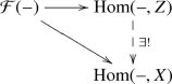
  is a coarse moduli space for \(\mathcal F \) (or X coarsely represents \(\mathcal F \)) if there exists a natural transformation \(\Phi :\mathcal F (-) \rightarrow {{\,\mathrm{Hom}\,}}(-,X)\) which satisfies:
-
(i)
 is bijective if k is algebraically closed (and \({{\,\mathrm{char}\,}}k =0\)); and
 -
(ii)
\(\Phi \) is universal: if \((Z,\Psi )\) is another such coarse moduli space, then there is a unique commutative diagram
 is bijective if k is algebraically closed (and
By Yoneda’s lemma, condition (ii) is equivalent to a unique (commuting) morphism \(X \rightarrow Z\).
We then define a functor  which associates to S the set of isomorphism classes of abelian schemes A over S—which can be thought of families of abelian surfaces parametrized by S—together with a map \(\iota :\mathcal {O}\hookrightarrow {{\,\mathrm{End}\,}}_S(A)\).
Deligne [Del71] has shown that the functor \(\mathcal F _\mathcal {O}\) is coarsely representable by a curve \(X_\mathbb Q ^1\) over \(\mathbb Q \). By uniqueness and the solution to the moduli problem over \(\mathbb C \), there is a map  which is in fact an analytic isomorphism. Together with the field of definition of CM points, we recover the canonical model (Theorem 43.8.1).
9 \(*\) Modular forms
In this final section, we sketch aspects of the theory of modular forms for arithmetic Fuchsian groups.
We restore a bit more generality: let F be a totally real field of degree \(n=[F:\mathbb Q ]\), let B be a quaternion algebra over F that split at exactly one real place corresponding to an embedding \(\iota _\infty :B \hookrightarrow {{\,\mathrm{M}\,}}_2(\mathbb R )\), let \(\mathcal {O}\subset B\) be an order, and let \(\Gamma \le {{\,\mathrm{PSL}\,}}_2(\mathbb R )\) be a group commensurable with \(\Gamma ^1(\mathcal {O}) = \iota _\infty (\mathcal {O}^1)/\{\pm 1\}\).
Let \(Y = \Gamma \backslash \mathbf{\textsf {H} }^2\), let \(X = \Gamma \backslash \mathbf{\textsf {H} }^{2(*)}\) be its completion, and call the set \(X \smallsetminus Y\) the set of cusps. We recall the notion of orbifold from section 34.8. Then X has the structure of a good complex 1-orbifold with signature \((g;e_1,\dots ,e_r;\delta )\): X has genus g, there are exactly r elliptic points \(P_i\) of orders \(e_i\), and \(\delta \) cusps \(Q_1,\dots ,Q_\delta \). The hyperbolic area of X is written \(\mu (X)\), and can be computed as the area of a suitable fundamental domain.
As in the introduction 43.1.6, we make the following definition.
Definition 43.9.1
Let \(k \in 2\mathbb Z _{\ge 0}\). A map \(f:\mathbf{\textsf {H} }^2\rightarrow \mathbb C \) is weight k -invariant under \(\Gamma \) if
A modular form for \(\Gamma \) of weight k is a holomorphic function \(f:\mathbf{\textsf {H} }^2\rightarrow \mathbb C \) that is weight k invariant and is holomorphic at the cusps.
Let \(M_k(\Gamma )\) be the \(\mathbb C \)-vector space of modular forms for \(\Gamma \) and let
then \(M(\Gamma )\) is a graded \(\mathbb C \)-algebra under multiplication.
We can understand the degree of divisors of \(M_k(\Gamma )\) as follows.
Theorem 43.9.4
For \(f \in M_k(\Gamma )\), we have
Proof See Shimura [Shi71, Proposition 2.16, Theorem 2.20].
By an application of the theorem of Riemann–Roch and the description of modular forms behind Theorem 43.9.4, we find that \(\dim _\mathbb C M_k(\Gamma )\) can be expressed in terms of k and the signature of \(\Gamma \) as follows.
Theorem 43.9.5
We have
Proof See Shimura [Shi71, Theorem 2.23].
The above formulas can be proven in a different and straightforward way in the language of stacky curves. This description gives the following further information on \(M(\Gamma )\).
Theorem 43.9.6
(Voight–Zureick-Brown [VZB2015]). Let \(e=\max (1,e_1,\dots ,e_r)\). Then the ring \(M(\Gamma )\) is generated as a \(\mathbb C \)-algebra by elements of weight at most 6e with relations in weight at most 12e.
(The case of signature (0; 2, 2, 3, 3; 0) from section 43.2 is described [VZB2015, Table (IVa-3)] as a weighted plane curve of degree 12 in \(\mathbb P (6,3,2)\).)
Remark 43.9.7. An appealing mechanism for working explicitly with modular forms in the absence of cusps is provided by power series expansions: for an introduction with computational aspects, see Voight–Willis [VW2014] and the references therein.
Exercises
-
1.
Let \(g=1\) and consider a period matrix \(\Pi =\begin{pmatrix} \omega _1&\omega _2 \end{pmatrix}\) with \(\omega _1,\omega _2 \in \mathbb C \). Let \(E=\begin{pmatrix} 0 &{} 1 \\ -1 &{} 0 \end{pmatrix}\). Show that in Definition 43.4.5 for E that the condition (i) is automatic and condition (ii) is equivalent to \({{\,\mathrm{Im}\,}}(\omega _2/\omega _1)>0\).
-
2.
Let \(\Pi \in {{\,\mathrm{Mat}\,}}_{g \times 2g}(\mathbb C )\). Show that \(\Pi \) is a period matrix for a complex torus if and only if \(\begin{pmatrix} \Pi \\ \overline{\Pi } \end{pmatrix}\), the matrix obtained by vertically stacking \(\Pi \) on top of its complex conjugate \(\overline{\Pi }\), is nonsingular.
-
3.
Let \(E :\Lambda \times \Lambda \rightarrow \mathbb Z \) be a \(\mathbb Z \)-bilinear form that satisfies conditions (i) and (ii) of Definition 43.4.9 (so a Riemann form but without the condition that E is alternating). Show that \(E_\mathbb{R }\) (and E) are alternating.
-
4.
Show that the symmetry (43.6.19) implies the equality
$$\begin{aligned} E\left( ix{\begin{pmatrix} \tau \\ 1 \end{pmatrix}}, iy{\begin{pmatrix} \tau \\ 1 \end{pmatrix}}\right) = E\left( x{\begin{pmatrix} \tau \\ 1 \end{pmatrix}}, y{\begin{pmatrix} \tau \\ 1 \end{pmatrix}}\right) \end{aligned}$$from (43.6.18) directly using Exercise 43.3 (without \(\varrho \)).
- \(\triangleright \)5.:
-
Let \(A=V/\Lambda \) be a complex abelian variety.
- (a):
-
Let \(\phi :A \rightarrow A'\) be an isogeny with \(n=\#\ker (\phi )\). Show that there exists a unique isogeny \(\psi :A' \rightarrow A\) such that \(\psi \circ \phi =n_A\) is multiplication by n on A and similarly \(\phi \circ \psi =n_{A'}\) on \(A'\). [Hint: \(\ker \phi \subseteq A[n]\).]
- (b):
-
Suppose that A is (not necessarily principally) polarized and let
 be the map induced by (43.4.20). Using (a), show that (43.4.22) gives a well-defined involution on \({{\,\mathrm{End}\,}}(A) \otimes \mathbb Q \), still called the Rosati involution (attached to the polarized abelian variety A).
- \(\triangleright \)6.:
-
Let V be a finite-dimensional vector space over \(\mathbb C \).
- (a):
-
Let \(H:V \times V \rightarrow \mathbb C \) be a nondegenerate Hermitian form on V. Let \(S:={{\,\mathrm{Re}\,}}H\) and \(E:={{\,\mathrm{Im}\,}}H\), so that \(H = S + iE\) for \(\mathbb R \)-bilinear forms \(S,E :V \times V \rightarrow \mathbb R \). Show that S is symmetric (i.e., \(S(y,x)=S(x,y)\)), E is alternating (i.e., \(E(y,x)=-E(x,y)\)), and \(S(x,y)=E(ix,y)\) for all \(x,y \in V\), and moreover that E (and S) are nondegenerate.
- (b):
-
Let E be a nondegenerate alternating form on V (as an \(\mathbb R \)-vector space). Show there exists a unique nondegenerate Hermitian form H on V with \({{\,\mathrm{Im}\,}}H = E\) if and only if \(E(ix,iy)=E(x,y)\) for all \(x,y \in V\).
- (c):
-
Show that a Hermitian form on V is positive definite if and only if the corresponding symmetric form \(S :={{\,\mathrm{Re}\,}}H\) is positive definite.
- \(\triangleright \)7.:
-
Prove Proposition 43.2.1.
- \(\triangleright \)8.:
-
In the following exercise, we do a few manipulations with generating functions, applied to understand the presentation of the ring of modular forms in the next exercise.
- (a):
-
Prove that
$$\begin{aligned} \sum _{k \in 2\mathbb Z _{\ge 2}} \left\lfloor \frac{k}{4}\right\rfloor t^k&= \frac{t^4}{(1-t^2)^2(1+t^2)} \\ \sum _{k \in 2\mathbb Z _{\ge 2}} \left\lfloor \frac{k}{3}\right\rfloor t^k&= \frac{t^4+t^6}{1-t^2-t^6+t^8} \end{aligned}$$[Hint: break up the sum by congruence class according to the floor and then use geometric series.]
- (b):
-
Let \(m_2,m_3 \in \mathbb Z _{\ge 0}\). For \(k \in 2\mathbb Z _{\ge 0}\), define
$$ c_k = {\left\{ \begin{array}{ll} 1, &{} \text { if }k=0; \\ g, &{} \text { if }k=2; \\ (k-1)(g-1) + m_2 \lfloor k/4\rfloor + m_3 \lfloor k/3 \rfloor , &{} \text { if }k \ge 4. \end{array}\right. } $$Show that
$$\begin{aligned} \sum _{k \in 2\mathbb Z _{\ge 0}} c_k t^k = \frac{1+gt^2+a_4t^4 + a_6t^6 + a_4t^8 + gt^{10}+t^{12}}{(1-t^4)(1-t^6)} \end{aligned}$$where
$$\begin{aligned} a_4&= 3g+m_2+m_3-4 \\ a_6&= 4g+m_2+2m_3-6. \end{aligned}$$
- \(\triangleright \)9.:
-
Prove Proposition 43.2.7 as follows.
- (a):
-
Show that the functions \(f_4,f_6\) are algebraically independent. [Hint: reduce to the case where the relation is weighted homogeneous, and plug in \(z_2\) to show the relation reduces to one of smaller degree.]
- (b):
-
Show that any relation between \(f_4,g_6,h_{12}\) is a multiple of r. [Hint: Without loss of generality, we may suppose that r is of the form \(h_{12}^2 \in \mathbb C [f_4,g_6]_{24}\). Therefore, another relation expresses \(h_{12}\) as a rational function in \(f_4,g_6\). Use (a) and unique factorization to show that this purported relation is in fact polynomial, and obtain a contradiction from the linear independence of \(f_4^3,g_6^2,h_{12}\).]
- (c):
-
Show that the subring of \(M(\Gamma ^1)\) generated by \(f_4,g_6,h_{12}\) is isomorphic to
$$\begin{aligned} M'=\mathbb C [f_4,g_6,h_{12}]/\langle r(f_4,g_6,h_{12}) \rangle . \end{aligned}$$ - (d):
-
Show that
$$\begin{aligned} \sum _{k \in 2\mathbb Z _{\ge 0}} (\dim _\mathbb C M_k(\Gamma ^1))t^k = \frac{1+t^{12}}{(1-t^4)(1-t^6)} \end{aligned}$$and \(\dim _\mathbb C M_k = \dim _\mathbb C M_k'\) for all k. [Hint: use Exercise 43.8.]
- (f):
-
Conclude that the subring of \(M(\Gamma ^1)\) generated by \(f_4,g_6,h_{12}\) is equal to \(M(\Gamma ^1)\). [Hint: Suppose that equality does not hold, and consider the minimal degree with a new generator; by dimensions, there must be a new relation, but argue that this relation must be among \(f_4,g_6,h_{12}\), contradicting (b).]
 be the map induced by (
Author information
Authors and Affiliations
Corresponding author
Rights and permissions
This chapter is distributed under the terms of the Creative Commons Attribution 4.0 International License (http://creativecommons.org/licenses/by/4.0/), which permits use, duplication, adaptation, distribution and reproduction in any medium or format, as long as you give appropriate credit to the original author(s) and the source, a link is provided to the Creative Commons license and any changes made are indicated.The images or other third party material in this chapter are included in the work's Creative Commons license, unless indicated otherwise in the credit line; if such material is not included in the work's Creative Commons license and the respective action is not permitted by statutory regulation, users will need to obtain permission from the license holder to duplicate, adapt or reproduce the material.
Copyright information
© 2021 The Author(s)
About this chapter

Cite this chapter
Voight, J. (2021). QM abelian surfaces. In: Quaternion Algebras. Graduate Texts in Mathematics, vol 288. Springer, Cham. https://doi.org/10.1007/978-3-030-56694-4_43
Download citation
DOI: https://doi.org/10.1007/978-3-030-56694-4_43
Published:
Publisher Name: Springer, Cham
Print ISBN: 978-3-030-56692-0
Online ISBN: 978-3-030-56694-4
eBook Packages: Mathematics and StatisticsMathematics and Statistics (R0)