
Abstract
In this chapter, we present an idelic formulation of zeta functions associated to central simple algebras over global fields and we prove that they have analytic continuation and functional equation.
You have full access to this open access chapter, Download chapter PDF
In this chapter, we present an idelic formulation of zeta functions associated to central simple algebras over global fields and we prove that they have analytic continuation and functional equation.
To read beyond the first two introductory sections, the additional prerequisite of real analysis at the level of measure theory is recommended; happily, the statements of the essential conclusions (for example, the functional equation of the zeta function of a quaternion algebra) can be understood without this background.
1 \(\triangleright \) Poisson summation and the Riemann zeta function
We begin with some essential motivation. Recall that the Riemann zeta function \(\zeta (s) :=\sum _{n=1}^{\infty } n^{-s}\) defined in (25.2.2). Following Riemann, we complete to the function \(\xi (s) :=\zeta (s)\Gamma _\mathbb R (s)\), where
and \(\Gamma (s)\) is the complex \(\Gamma \)-function (Exercise 26.2). Then \(\xi (s)\) extends to a meromorphic function on \(\mathbb C \) and satisfies the functional equation
(More generally, we saw in 26.8.2 that the Dedekind zeta function of a number field can be completed in an analogous manner, again with functional equation.)
In this introductory section, we sketch a proof of the functional equation and see it as a consequence of Poisson summation (arising naturally in Fourier analysis, still following Riemann). Then, following Tate we reinterpret this extra factor in a manner that realizes the zeta function as a zeta integral on an adelic space, giving a uniform description and making the whole setup more suitable for analysis.
To begin, we the function \(\xi (s)\) itself as an integral. Looking at one term in \(\xi (s)\), we have
Accordingly, we define the theta function
studied by Jacobi, convergent absolutely to a holomorphic function on the right half-plane \({{\,\mathrm{Re}\,}}u>0\). Summing over \(n \ge 1\) gives
valid for \({{\,\mathrm{Re}\,}}s > 1\), where the integral converges (so we may justify interchanging summation and integration). We will soon rewrite this integral so as to extend its definition to all \(s \in \mathbb C \) apart from \(s=0,1\).
Let \(f:\mathbb R \rightarrow \mathbb C \) be a Schwartz function, so f is infinitely differentiable and every derivative decays rapidly (for all \(m,n \ge 0\) we have \(|f^{(m)}(x) \,|=O(x^{-n})\) as \(|x \,| \rightarrow \infty \)). We define the Fourier transform  of f by

Theorem 29.1.7
(Poisson summation). We have

with both sums converging absolutely.
Proof. The condition that f is Schwartz ensures good analytic behavior allowing the interchange of sum and integral, the details of which we elide. Let \(g(x) :=\sum _{m=-\infty }^{\infty } f(x+m)\). Then g is periodic with period 1, so by Fourier expansion we have \(g(x)=\sum _{n=-\infty }^{\infty } a_n e^{2\pi i n x}\) where

Thus

Now take \(f(x)=e^{-\pi x^2}\). Then f is Schwartz. By contour integration and using \(\int _{-\infty }^{\infty } e^{-\pi x^2}\,\mathrm{d }{x} = 1\), we conclude that  for all y. For \(u>0\), let \(f_u(x) :=f(ux)\); then
  by change of variable. Applying Poisson summation to \(f_{\sqrt{u}}(x)\) then gives
The equation (29.1.9) implies the functional equation (29.1.2) for \(\xi (s)\) as follows: we split up the integral (29.1.5) as
and apply the change of variable \(u \leftarrow 1/u\) to obtain
Putting these together, we have
which is sensible as a meromorphic function for all \(s \in \mathbb C \), holomorphic except for \(s=0,1\), with the right-hand side visibly invariant under \(s \leftarrow 1-s\). This establishes (29.1.2).
This method extends to prove the functional equation for the L-series \(L(s,\chi )\) where \(\chi \) is a Dirichlet character (now involving a Gauss sum); Hecke extended this method (generalizing the appropriate theta functions) to prove the functional equation for a wider class of functions, including the Dedekind zeta functions.
2 \(\triangleright \) Idelic zeta functions, after Tate
Now convinced of the utility of integral representations, we seek to put the finite places on an equal footing. In this way, the inclusion \(\mathbb Z \subseteq \mathbb R \) in the Fourier analysis above is replaced by \(\mathbb Q \subseteq \underline{\mathbb{Q }}\). Recall that \(\zeta (s)=\prod _p \zeta _p(s)\) where
we recover these factors from an integral. First we need a measure to integrate against. We have \(\mathbb Z _p = \varprojlim _n \mathbb Z /p^n \mathbb Z \) as a projective limit with compatible projection maps \(\pi _n:\mathbb Z _p \rightarrow \mathbb Z /p^n\mathbb Z \). We define the measure on \(\mathbb Z _p\) as the projective limit of the counting measures on each \(\mathbb Z /p^n \mathbb Z \) with total measure 1, i.e., for a set \(E \subseteq \mathbb Z _p\) we define
when this limit exists. The measure extends additively to \(\mathbb Q _p=\mathbb Z _p[1/p]\) and is invariant under additive translation
accordingly, \(\mu _p\) is the standard Haar measure on \(\mathbb Q _p\) (see 29.3). We have normalized the measure so that
Since \(\mathbb Z _p^\times = \mathbb Z _p \smallsetminus p\mathbb Z _p\) and \(\mathbb Z _p = \bigsqcup _{a=0}^{p-1} (a + p\mathbb Z _p)\) we have \(\mu (p\mathbb Z _p)=1/p\) and
Similarly, we have a standard Haar measure \(\mu _p^\times \) on \(\mathbb Q _p^\times \) by
the measure is invariant under \(x \leftarrow ax\) for \(a \in \mathbb Q _p^\times \) as well as under the substitution \(x \leftarrow x^{-1}\), and with our normalization we have
For a complex number \(s \in \mathbb C \), on our way to recover \(\zeta _p(s)\) we consider the (Lebesgue) integral
This looks a bit weird at first, because it is not over a subgroup of \(\mathbb Q _p^\times \) or anything. Nevertheless, it works! For every nonzero \(x \in \mathbb Z _p \smallsetminus \{0\}\), we may write \(x=p^e x_0\) with \(x_0 \in \mathbb Z _p^\times \) and \(e \ge 0\), therefore the integral can be written as a sum over the level sets \(p^e \mathbb Z _p^\times \):
It is more common to rewrite this as an integral over \(\mathbb Q _p^\times \) by letting \(\Psi _p\) be the characteristic function of \(\mathbb Z _p \smallsetminus \{0\}\), so that
In a similar fashion, we define the measure \(\mu _\infty \) on \(\mathbb R \) by \(\mathrm{d }{x}/|x \,|\), and to match (29.1.1) we define \(\Psi _\infty (x)=e^{-\pi x^2}\). Putting these together, on the idele group \(\underline{\mathbb{Q }}^\times \) we define the product measure \(\mu ^\times = \prod _v \underline{\mu }_v^\times \), the function \(\underline{\Psi }(\underline{x})=\prod _v \Psi _v(x_v)\), and absolute value \(\left\| {\underline{x}}\right\| =\prod _v |x_v \,|_v\) (trivial on \(\mathbb Q ^\times \) by the product formula). We have then repackaged the zeta function as an adelic integral
This is really nice!
Rewritten in this idelic way, Tate [Tate67] in his Ph.D. thesis elegantly proved the functional equation for a wide class of zeta functions (and L-functions):
[T]he role of Hecke’s complicated theta-formulas for theta functions formed over a lattice in the n-dimensional space of classical number theory can be played by a simple Poisson formula [...], the number theoretic analogue of the Riemann–Roch theorem” [Tate67, p. 305–306].
In this chapter, we use this method of Poisson summation and idelic integrals to prove the basic properties of the zeta function of a central simple algebra over a global field (Main Theorem 29.10.1). Translated back into classical language, we prove as a consequence the key result (the crux of which is Theorem 26.8.19) announced in section 26.8.
Main Theorem 29.2.6
Let F be a number field with ring of integers \(R=\mathbb Z _F\) and let B be a quaternion algebra over F with maximal order \(\mathcal {O}\). Let

be the sum over nonzero right \(\mathcal {O}\)-ideals, where  is the absolute (counting) norm (16.4.7) and let \(\xi _B(s)\) be its completion (26.8.13). Then \(\xi _B(s)\) has meromorphic continuation to \(\mathbb C \), holomorphic away from \(\{0,1/2,1\}\) with simple poles at \(s=0,1\), and it satisfies the functional equation
Moreover, if B is a division algebra, then \(\xi _B(s)\) is holomorphic at \(s=1/2\).
Main Theorem 29.2.6 is an analytic result with key arithmetic consequences, including the classification of quaternion algebras over global fields, as we saw in section 26.8. More than that, the evaluation of the residue will further give rise to a volume formula (Main Theorem 39.1.8) that generalizes the Eichler mass formula (as in the proof of Proposition 26.5.10).
The developments in this chapter have a rich history, and they generalize vastly beyond this text: see Remark 29.10.24. We restrict ourselves to the case of zeta functions both because this suffices for our main applications and because it is a good stepping stone to the more general theory. Although this chapter is quite technical, the reader’s forbearance will ultimately be rewarded!
3 Measures
In this section, we define the local measures we will use. As references for this section and the next, see Bekka–de la Harpe–Valette [BHV2008, Appendices A and B], Deitmar [Dei2005], Deitmar–Echterhoff [DE2009, Chapters 1 and 3, Appendix B], Loomis [Loo53], and Ramakrishnan–Valenza [RM99, Chapters 1–4] as references on harmonic analysis, and Vignéras [Vig80a, §II.4] and Weil [Weil74, Chapter XI] for the present context.
Let G be a Hausdorff, locally compact, second countable topological group. For example, we may take \(G={{\,\mathrm{SL}\,}}_2(\mathbb R )\) or \(G={{\,\mathrm{SL}\,}}_n(\mathbb R )\) (or more generally a semisimple real Lie group). A Borel measure on G is a countably additive function, with values in \([0,\infty ]\), defined on the \(\sigma \)-algebra generated by open sets in G under complement and finite or countable unions.
Definition 29.3.1
A Radon measure on G is a Borel measure that is finite on compact sets. A left Haar measure on G is a nonzero Radon measure \(\mu \) that is left translation-invariant, so \(\mu (gE)=\mu (E)\) for all Borel subsets \(E \subseteq G\) and all \(g \in G\).
The notion of right Haar measure is defined similarly.
Remark 29.3.2. Since G is second countable and locally compact, every open subset of G is \(\sigma \) \(\sigma \) -compact (the union of a countable collection of compact subspaces), so a Radon measure is necessarily regular, i.e., the measure of a Borel set is the infimum of the measures of its open supersets and the measure of an open set is the supremum of the measures of its compact subsets: see Rudin [Rud87, Theorem 2.18].
Proposition 29.3.3
G admits a left Haar measure that is unique up to scaling by an element of \(\mathbb R _{>0}\).
Proof. See e.g. Deitmar–Echterhoff [DE2009, Theorem 1.3.4] or Diestel–Spalsbury [DS2014, §7.2].□
We will construct Haar measures explicitly as we need them, so we need not appeal to the general result of Proposition 29.3.3 beyond the uniqueness statement which is itself straightforward to establish: see Exercise 29.4.
Example 29.3.4
On \(G=\mathbb R ^n\) under addition, a left (and right) Haar measure is given by the usual Lebesgue measure.
Example 29.3.5
Suppose G has the discrete topology (all sets are open). Then the counting measure \(\mu (E)=\#E \in \mathbb Z _{\ge 0} \cup \{\infty \}\) is a left (and right) Haar measure.
From now on, let \(\mu \) be a left Haar measure on G.
29.3.6
In general, a left Haar measure need not also be right translation-invariant. For \(g \in G\), the measure defined by \(\mu _g(E) :=\mu (Eg)\) for a Borel set E is again a left Haar measure, so by Proposition 29.3.3, we have \(\mu _g = \Delta _G(g) \mu \) for some \(\Delta _G(g) \in \mathbb R _{>0}\). Since \(\mu \) is unique up to scaling, the function \(\Delta _G(g)\) does not depend on \(\mu \).
Definition 29.3.7
The map \(\Delta _G :G \rightarrow \mathbb R _{>0}\) is the modular function of G. We say G is unimodular if \(\Delta _G\) is identically 1.
By 29.3.6, G is unimodular if and only if every left Haar measure is a right Haar measure.
Lemma 29.3.8
The modular function \(\Delta _G\) is a homomorphism.
Proof. Exercise 29.5.□
Example 29.3.9
If G is abelian or discrete (see Example 29.3.5), then G is unimodular: every left Haar measure is a right Haar measure. (There are many other important classes of groups that are unimodular, including discrete (e.g., finite) groups, compact groups, and the others we will in what follows.)
29.3.10
In this paragraph, we briefly review the theory of integration we need; for further details, see Deitmar–Echterhoff [DE2009, Appendix B.1]. Let \(f:G \rightarrow \mathbb C \) be a complex-valued function on G. We say f is measurable if for all Borel sets \(E \subseteq \mathbb C \), the subset \(f^{-1}(E)\) is measurable; we say f is real(-valued) if \(f(G) \subseteq \mathbb R \) and is nonnegative if \(f(G) \subseteq \mathbb R _{\ge 0}\).
If E is a measurable set then the characteristic function \(1_E\) of E (equal to 1 on E and 0 outside E) is defined to have integral
A step function is a finite \(\mathbb C \)-linear combination of characteristic functions of measurable sets, and we define the integral of a step function by linearity using (29.3.11).
If f is measurable and nonnegative, we define

and say f is integrable if \(\int _G f(x)\,\mathrm{d }{\mu (x)}<\infty \).
If f is real we say f is integrable if both \(f^+ :=\max (f,0)\) and \(f^- :=-\min (f,0)\) are integrable. If f is real and integral, we then define
Finally, a general f is integrable if \({{\,\mathrm{Re}\,}}f\) and \({{\,\mathrm{Im}\,}}f\) are integrable, in which case
29.3.13
Let H be another Hausdorff, locally compact, second countable topological group, and let \(\phi :G \rightarrow H\) be continuous surjection with kernel \(N :=\ker \phi \). Then we have an exact sequence
We say that left Haar measures on G, N, H are compatible if for all integrable functions \(f:G \rightarrow \mathbb C \),
Given measures on two terms, there exists a unique compatible measure on the third—but note, this measure depends on the exact sequence (Exercise 29.7).
4 Modulus and Fourier inversion
We continue our background review with notation from the previous section; we now treat the modulus of an automorphism and present Fourier inversion.
29.4.1
Let \(\phi \in {{\,\mathrm{Aut}\,}}(G)\) be a continuous automorphism. Then the measure defined by \(\mu _\phi (E) :=\mu (\phi (E))\) is again a left Haar measure. By Proposition 29.3.3, there exists a unique \(\left\| {\phi }\right\| \in \mathbb R _{>0}\) such that
for all measurable sets E. In particular, for all integrable functions f on G we have
Definition 29.4.4
The modulus of \(\phi \in {{\,\mathrm{Aut}\,}}(G)\) is \(\left\| {\phi }\right\| \in \mathbb R _{>0}\) as defined in (29.4.2).
The definition of the modulus is independent of the choice of Haar measure \(\mu \), since Haar measure is unique up to scaling and such a scalar cancels in (29.4.2).
Example 29.4.5
Let \(g \in G\); then the conjugation automorphism \(\phi _g(x)=g^{-1}xg\) has \(\left\| {\phi _g}\right\| =\Delta _G(g)\), because \(\mu \) is left-invariant. In particular, G is unimodular if and only if all conjugation maps have trivial modulus.
Now let A be a Hausdorff, locally compact, second countable topological ring and let \(\mu \) be a left Haar measure on the additive group of A. Since A is abelian, A is unimodular and \(\mu \) is also a right Haar measure.
29.4.6
Let \(a \in A^\times \). Then the left multiplication map \(\lambda _a:A \rightarrow A\) by \(x \mapsto ax\) is a continuous automorphism of A as an additive abelian group, so we may define its modulus \(\left\| {a}\right\| :=\left\| {\lambda _a}\right\| \) by (29.4.2): symbolically, we write
We have \(\left\| {ab}\right\| =\left\| {a}\right\| \left\| {b}\right\| \) for all \(a,b \in A^\times \) (Exercise 29.6).
29.4.8
The measure on \(A^\times \) defined by
is a (multiplicative) Haar measure by 29.4.6.
We conclude this introductory section with the Fourier inversion formula.
29.4.10
Let \(\mathbb C ^1 :=\{z \in \mathbb C : |z \,|=1\}\) be the circle group. A unitary character of A is a continuous homomorphism \(\chi :A \rightarrow \mathbb C ^1\), considering A as an additive group. Let  be the unitary character group of A under pointwise multiplication, and equip
  with the compact-open topology (as a closed subset of the set of all continuous maps \(A \rightarrow \mathbb C ^1\)).
Remark 29.4.11. We reserve the term character for continuous group homomorphisms \(A \rightarrow K^\times \), where K is a field (of values for the character); this notion makes sense for any field K. Some authors call unitary characters just characters, then calling our characters instead quasi-characters.
Now suppose that there exists  such that the map

is an isomorphism of topological groups. (This is a hypothesis on A, and may depend on a choice; in the cases we consider below, we will identify a standard such \(\psi \).)
Definition 29.4.12
For \(f:A \rightarrow \mathbb C \) continuous and integrable, the Fourier transform of f (relative to \(\psi ,\mu \)) is the function

Theorem 29.4.13
(Fourier inversion). There exists a unique Haar measure \(\tau \) on A (depending on \(\psi \)) such that for all \(f:A \rightarrow \mathbb C \) continuous and integrable with  (defined relative to \(\tau \)) continuous and integrable, we have

Proof. The proof of this theorem is beyond the scope of this textbook, and we use it as a black box; see e.g. Deitmar–Echterhoff [DE2009, Theorem 3.5.8] or Folland [Fol95, Theorems 4.32–4.33].□
The normalized measure \(\tau \) in Theorem 29.4.13 is called the self-dual measure on A (with respect to \(\psi \)).
5 Local measures and zeta functions: archimedean case
Let B be a finite-dimensional simple algebra over the local field \(F=\mathbb R \). A good general reference for the next three sections is Weil [Weil82, Chapter II].
29.5.1
The (additive) Haar measure \(\mu \) on B is the usual (Lebesgue) measure, normalized as follows: letting \(n=\dim _\mathbb R B\), we choose an \(\mathbb R \)-basis \(e_1,\dots ,e_n\) for B, so that we may write \(x=\sum _i x_i e_i \in B\) with \(x_i\) are coordinates on B, and we define
where d is the discriminant defined by (15.2.1) and the reduced trace is taken on B as an \(\mathbb R \)-algebra. By Lemma 15.2.5, we see that this measure is independent of the choice of basis \(e_i\).
Another application of Lemma 15.2.5 then gives the modulus
for all \(\alpha \in B^\times \).
Example 29.5.3
We compute:
And:
The modulus for \(\mathbb R \) is the usual absolute value, whereas the modulus for \(\mathbb C \) is the square of the absolute value (cf. Remark 12.2.3), explaining conventions on normalized absolute values in the product formula 14.4.6.
29.5.4
As in (29.4.9), the (multiplicative) Haar measure \(\mu ^\times \) on \(B^\times \) is defined by
29.5.6
We define the standard unitary character
with reduced trace taken on B as an \(\mathbb R \)-algebra. We note that \(\psi (\alpha \beta )=\psi (\beta \alpha )\) for all \(\alpha ,\beta \in B\).
A fundamental result in standard Fourier analysis (generalizing the case \(B=\mathbb R ,\mathbb C \) and following from it in the same way) is the following proposition.
Proposition 29.5.7
The standard unitary character induces an isomorphism  of topological groups, and the measure \(\mu \) defined in 29.5.1 is self-dual (with respect to \(\psi \)).
In light of Proposition 29.5.7, we will also write \(\tau =\mu \) for the measure defined above.
29.5.8
The exact sequence
defines a measure \(\tau ^1\) on \(\mathbb H ^1\) by compatibility, taking the normalized measures \(\tau ^\times \) on \(\mathbb H ^\times \) and on \(\mathbb R _{>0} \le \mathbb R ^\times \).
Lemma 29.5.9
We have \(\tau ^1(\mathbb H ^1) = 4\pi ^2\).
Proof. Let \(\rho >0\) and let
be the punctured ball of radius \(\rho \). Let f be the function \(\left\| {\alpha }\right\| \) on E, zero elsewhere. On the one hand,
Recalling that \(\tau \) is 4 times Lebesgue measure, and that the Lebesgue measure of a sphere of radius \(\rho \) has volume \(\pi ^2\rho ^4/2\), we get \(\tau (E) = 2\pi ^2\rho ^4\). On the other hand, by compatibility, this integral is equal to
We conclude that \(\tau ^1(\mathbb H ^1) = 4\pi ^2\).□
We will need further functions to integrate, so we make the following definition. When we consider functions on B, we may think of choosing an \(\mathbb R \)-basis \(e_1,\dots ,e_n\) of B, identifying \(B \simeq \mathbb R ^n\) and writing \(x=\sum _i x_i e_i \in B\); our definitions will be independent of this choice of basis.
Definition 29.5.10
A function \(f:B \rightarrow \mathbb C \) decays rapidly if for all \(n \ge 0\) we have \(|f(x) \,|=O((\max _i |x_i \,|)^{-n})\) as \(\max _i |x_i \,| \rightarrow \infty \).
A function \(f:B \rightarrow \mathbb C \) is Schwartz(–Bruhat)if f is infinitely differentiable and every partial derivative of f decays rapidly.
29.5.11
Let \({}^*:B \rightarrow B\) be the conjugate transpose involution (see 8.4.3) on B. Let \(Q(\alpha ) :={{\,\mathrm{trd}\,}}(\alpha \alpha ^*)\) for \(\alpha \in B\). We compute that
Definition 29.5.13
The standard function on B is
It is straightforward to verify that the standard function is Schwartz.
Definition 29.5.15
For a Schwartz function \(\Phi \), we define the (local) zeta function
wherever this integral converges. We abbreviate \(Z_B^{\Psi }(s)=Z_B(s)\) for \(\Phi =\Psi \) the standard function.
As in (26.8.3), we define
Lemma 29.5.18
We have
Proof. We have
making the substitution \(x \leftarrow \pi x^2\) gives the result. A similar argument with polar coordinates gives \(Z_\mathbb{C }(s)\). The remaining integrals are pretty fun, so they are left as Exercise 29.8.□
Lemma 29.5.18 explains the provenance of the definitions of \(\Gamma _\mathbb R (s),\Gamma _\mathbb C (s)\) from (26.8.3), and ultimately their appearance in (26.8.14). (A quick check on the constant in front is provided by \(Z_B(1)=1\); these particular choices of constants follow convention.) By comparison, Lemma 29.5.18 then shows that in general \(Z^{\Phi }_B(s)\) has meromorphic continuation to \(\mathbb C \).
6 Local measures: commutative nonarchimedean case
Now let F be a nonarchimedean local field, with valuation v, valuation ring R, and maximal ideal \(\mathfrak p =\pi R \subseteq R\). Let \(q :=\#R/\mathfrak p \).
We begin by defining a Haar measure normalized so that R has measure 1; then we extend this to find the normalization in which the measure is self-dual with respect to a standard unitary character.
29.6.1
We have \(R \cong \varprojlim _n R/\mathfrak p ^n\) with projection maps \(\pi _n :R \rightarrow R/\mathfrak p ^n\). We define the (additive) measure \(\mu \) on R by
for a subset \(E \subset R\), when this limit exists. It is straightforward to check that E defines a Haar measure on R, and the measure extends to F by additivity. In this normalization, we have \(\mu (R)=1\), and more generally \(\mu (a+\mathfrak p ^n)=1/q^n\) for \(a \in R\) and \(n \ge 0\).
Let \(|\phantom {.} \,|\) be the preferred absolute value (see 14.4.12), with \(|\pi \,|=1/q\).
Lemma 29.6.2
For all \(x \in F^\times \), we have
in particular, if \(x \in R\), then \(|x \,|=\mathsf N (Rx)^{-1}\) where \(\mathsf N \) is the counting norm (16.4.7).
Proof. By multiplicativity, we may suppose \(x \in R\). Then \([R:xR]=q^{v(x)}=\mathsf N (Rx)\). Adding up cosets of xR in R, we obtain
so \(\left\| {x}\right\| =\mu (xR)/\mu (R)=q^{-v(x)}=|x \,|\), as claimed.□
Example 29.6.4
Since \(\mu (R^\times )=\mu (R)-\mu (\mathfrak p )\) and
we have
29.6.6
We normalize the (multiplicative) Haar measure \(\mu ^\times \) on \(F^\times \) by defining
so that \(\mu ^\times (R^\times )=1\).
Next, we consider the Fourier transform in this context.
29.6.7
We first define an additive homomorphism
as follows.
-
(a)
If \(F=\mathbb Q _p\), we define \(\langle x \rangle _\mathbb{Q _p} \in \mathbb Q \) to be such that \(0 \le \langle x \rangle _\mathbb{Q _p} < 1\) and \(x-\langle x \rangle _\mathbb{Q _p} \in \mathbb Z _p\).
-
(b)
If \(F=\mathbb F _q((t))\) and \(x=\sum _i a_i t^i\) then we take \(\langle x \rangle _F :={{\,\mathrm{Tr}\,}}_\mathbb{F _q/\mathbb F _p}(a_{-1})/p\).
-
(c)
In general, if \(F \supseteq F_0\) is a finite separable extension of fields, then we define
$$\begin{aligned} \langle x \rangle _F :=\langle {{\,\mathrm{Tr}\,}}_{F/F_0} x \rangle _{F_0}. \end{aligned}$$
Definition 29.6.8
The standard unitary character of F is
Proposition 29.6.9
The standard unitary character \(\psi _F\) defines an isomorphism

of topological groups.
Proof. Exercise 29.9.□
Proposition 29.6.10
The following statements hold.
-
(a)
If F is a local number field (so a finite extension of \(\mathbb Q _p\) for a prime p), then the measure

is self-dual (with respect to \(\psi \)).
-
(b)
If F is a local function field, then \(\mu \) is self-dual with respect to \(\psi \).

Proof. First consider (a), and suppose F is a finite extension of \(\mathbb Q _p\). We seek to satisfy (29.4.14); the equation holds up to a constant, so we may choose appropriate f and x. We choose f as the characteristic function of R and \(x=0\), so that \(f(0)=1\) and
By character theory,
so (29.6.11) is equal to \(\mu (R^\sharp )\) where
Let \(x_i\) be a \(\mathbb Z _p\)-basis for R with \(x_i^\sharp \) the dual basis, giving a \(\mathbb Z _p\)-basis for \(R^\sharp \). By Lemma 15.6.17 we have
so since \(\mu (R)=1\) by additivity we have
It follows then that
is self-dual.□
7 Local zeta functions: nonarchimedean case
Continuing with F a nonarchimedean local field, let B be a finite-dimensional simple (not necessarily central) algebra over F, with maximal order \(\mathcal {O}\), and \(n^2=\dim _{Z(B)} B\).
29.7.1
The (additive) Haar measure \(\mu \) on B is defined as in 29.6.1 as a projective limit, normalized so that \(\mu (\mathcal {O})=1\).
We compute that \(\left\| {\alpha }\right\| _B=\left\| {{{\,\mathrm{Nm}\,}}_{B|F}(\alpha )}\right\| _F\), so that if B is central over F with \(\dim _F B=n^2\), then \(\left\| {\alpha }\right\| _B=\left\| {{{\,\mathrm{nrd}\,}}(\alpha )^n}\right\| _F\). In the remainder of this section, we work over B and drop the subscript \({}_B\).
29.7.2
For the (multiplicative) Haar measure \(\mu ^\times \) on \(B^\times \), we use the same normalization factor (29.6.5) as for \(F^\times \), defining the normalized measure
29.7.4
We extend the standard unitary character on F, defined in 29.6.7, to a standard unitary character on B by
for \(\alpha \in B\). Again, \(\psi (\alpha \beta )=\psi (\beta \alpha )\) for all \(\alpha ,\beta \in B\).
If F is a local number field containing \(\mathbb Q _p\), let \(R_0=\mathbb Z _p\); if F is a local function field, let \(R_0=R\).
Definition 29.7.5
The absolute discriminant of B is

The absolute discriminant is well-defined, independent of the choice of maximal order.
Example 29.7.6
If B is a quaternion algebra over F, then

Proposition 29.7.7
The standard unitary character \(\psi \) defines an isomorphism  of topological groups, and the measure

is self-dual with respect to \(\psi \).
Proof. The same arguments as in Propositions 29.6.9 and 29.6.10 apply, with appropriate modifications.□
29.7.9
Having normalized the multiplicative measure \(\mu ^\times \) and seeing the relevant modification in (29.7.8), just as in the case of \(B=F\) we define

We may now define the local zeta function in the nonarchimedean context.
Definition 29.7.11
A function \(f:B \rightarrow \mathbb C \) is Schwartz–Bruhat if f is locally constant (for every \(\alpha \in B\), there exists an open neighborhood \(U \ni x\) such that \(f|_U\) is constant) with compact support. A standard function \(\Psi \) on B is the characteristic function of a maximal order.
Taking an open cover of the support, we see that every Schwartz–Bruhat function can be expressed as a (finite) \(\mathbb C \)-linear combination of characteristic functions of compact open subsets of B.
Definition 29.7.12
For a Schwartz–Bruhat function \(\Phi \), we define the (local) zeta function
We write
for the zeta function with respect to a standard function \(\Psi \); this is well-defined (independent of \(\Psi \)) as any two maximal orders are conjugate, and \(\left\| {\alpha }\right\| \) is well-defined on conjugacy classes by 29.7.1.
We begin with a basic convergence estimate.
Lemma 29.7.15
The function \(Z_B^{\Phi }(s)\) converges for \({{\,\mathrm{Re}\,}}s>1\).
Proof. We reduce to the case where \(\Phi \) is the characteristic function of a compact open set U, since \(\Phi \) is a (finite) \(\mathbb C \)-linear combination of such. Since U is compact, \(\left\| {\alpha }\right\| \) is bounded on U, so too is \(\left\| {\alpha }\right\| ^{s-1}\) for fixed \({{\,\mathrm{Re}\,}}s>1\); thus
is bounded by a constant multiple of \(\tau (U)<\infty \), and therefore \(Z_B^{\Phi }(s)\) is bounded by comparison.□
This integral representation recovers the classical zeta function we studied earlier in the number field case (section 26.4).
29.7.16
Since there is a unique ideal in R of absolute norm \(q^e\) for each \(e \ge 0\), we have
In like fashion, for \(e \ge 0\), let \(a_\mathfrak{p ^e}=a_\mathfrak{p ^e}(\mathcal {O})\) be the number of (necessarily principal) right ideals of \(\mathcal {O}\) of reduced norm \(\mathfrak p ^e\) and thereby absolute norm \(q^{ne}\). We then define

the sum as usual over all nonzero right ideals of \(\mathcal {O}\).
Lemma 29.7.17
The following statements hold.
-
(a)
We have
$$\begin{aligned} Z_{B}(s) = \tau ^\times (\mathcal {O}^\times )\zeta _{B}(s); \end{aligned}$$in particular, the domain of convergence of \(Z_B(s)\) is the same as \(\zeta _B(s)\).
-
(b)
If B is a quaternion algebra, then \(\zeta _B(s)\) converges for \({{\,\mathrm{Re}\,}}s>1/2\), and
$$ \zeta _{B}(s) = {\left\{ \begin{array}{ll} \zeta _{F}(2s), &{} \text { if }B\text { is a division algebra;} \\ \zeta _{F}(2s)\zeta _{F}(2s-1), &{} \text { if }B \simeq {{\,\mathrm{M}\,}}_2(F). \end{array}\right. } $$ -
(c)
If \(B\simeq {{\,\mathrm{M}\,}}_n(F)\), then \(\zeta _B(s)\) converges for \({{\,\mathrm{Re}\,}}s>1-1/n\), and
$$\begin{aligned} \zeta _{B}(s)= \prod _{i=0}^{n-1} \zeta _F(ns-i). \end{aligned}$$
Proof. First part (a). For \(e \ge 0\), choose representatives for the \(a_\mathfrak{p ^e}=a_\mathfrak{p ^e}(\mathcal {O})\) classes in \(\mathcal {O}/ \mathcal {O}^\times \) with reduced norm \(\mathfrak p ^e\). Every element \(\alpha \in \mathcal {O}\cap B^\times \) can be written as the product of one of the representatives and an element of \(\mathcal {O}^\times \); since \(\left\| {\alpha }\right\| =|{{\,\mathrm{nrd}\,}}(\alpha )^n \,|\) we have
as claimed. For (b) and (c), we gave a formula for \(a_\mathfrak{p ^e}\) for \(B={{\,\mathrm{M}\,}}_n(F)\) in Exercise 26.12 and for B a quaternion algebra in Corollary 26.4.7 (which extends to the function field case without change). Of course, these identities only hold within their respective domains of convergence, which for \(\zeta _F(s)=(1-q^{-s})^{-1}\) is \({{\,\mathrm{Re}\,}}s>0\), thereby giving the rest.□
In the proof of the functional equation, we will need the following proposition, recalling duality (section 15.6).
Proposition 29.7.19
For \(\Psi \) the characteristic function of \(\mathcal {O}\), we have

Moreover,

Proof. For the first statement, by definition we have

If \(\alpha \in \mathcal {O}^\sharp \) then \(\psi (\alpha \beta )=1\) for all \(\beta \in \mathcal {O}\), and we obtain

Otherwise, \(\alpha \not \in \mathcal {O}^\sharp \), and by character theory  .
.
Since \(\mathcal {O}\) is maximal, we have \(\mathcal {O}^\sharp =\mathcal {O}\delta \) for some \(\delta \in B^\times \) with  . Therefore

□proving the second statement.
We conclude this section with some hopefully illustrative computations of measure.
Lemma 29.7.22
Let B be a quaternion algebra over F. Then
Proof. If B is a division ring, then \(\mathcal {O}\) is the valuation ring; let \(J \subseteq \mathcal {O}\) be the maximal ideal, so \(\mathcal {O}/J \simeq \mathbb F _{q^2}\) hence \(\mu (J)=1/q^2\), and then
Similarly, if \(B \simeq {{\,\mathrm{M}\,}}_2(F)\) then \(\mathcal {O}\simeq {{\,\mathrm{M}\,}}_2(R)\), and from the exact sequence
where \(k=R/\mathfrak p \), we compute \(\mu (1+\mathfrak p {{\,\mathrm{M}\,}}_2(R))=\mu (\mathfrak p {{\,\mathrm{M}\,}}_2(R))=1/q^4\) and

29.7.24
Let B be a quaternion algebra. Then the reduced norm yields an exact sequence
so we have an induced compatible measure \(\tau ^1\) on \(\mathcal {O}^1\). Thus

8 Idelic zeta functions
In this section, we now define (global) zeta functions in an idelic context. Let F be a global field and let B be a central simple algebra over F.
We first define the classical zeta function before generalizing to idelic zeta functions. We define
the product over all nonarchimedean places of the local zeta functions \(\zeta _{B_v}(s)\) defined in 29.7.16. We studied these (global) zeta functions over number fields in Chapters 25 and 26.
Example 29.8.2
By Lemma 29.7.17(c) we have
With this in mind, we construct idelic zeta functions as products of local zeta functions, according to the product measures and characters, as follows.
29.8.3
For \(v \in {{\,\mathrm{Pl}\,}}F\), we have defined measures \(\mu _v\) on \(B_v\) in 29.5.1 for v archimedean and 29.7.1 for v nonarchimedean. We define the measure
on \(\underline{B}\) as the product measure (on the restricted direct product). In particular, for every eligible set \({{{\texttt {\textit{S}}}}}\subset {{\,\mathrm{Pl}\,}}F\) of places and every \(R_{({{{\texttt {\textit{S}}}}})}\)-order \(\mathcal {O}\) in B, the measure \(\underline{\mu }\) restricts to the (convergent) product measure on \(\prod _{v \in {{{\texttt {\textit{S}}}}}} B_v \times \prod _{v \not \in {{{\texttt {\textit{S}}}}}} \mathcal {O}_v\)—and this uniquely defines the \(\underline{\mu }\) as a Haar measure on \(\underline{B}\).
Definition 29.8.4
The absolute discriminant  of B is defined as the product of the local absolute discriminants over all nonarchimedean places:

The absolute discriminant is well-defined because  for all but finitely many v.
Example 29.8.5
If F is number field, let \(d_F \in \mathbb Z \) be the discriminant of F. Multiplying the factors 29.7.6 together, if B is a quaternion algebra we find that

the product taken over all nonarchimedean ramified places.
29.8.6
In light of Proposition 29.7.7, we define the Tamagawa measure on \(\underline{B}\) by

with \(\tau _v=\mu _v\) for v archimedean and  defined in (29.7.8) for v nonarchimedean.
Remark 29.8.8. The Tamagawa measure has an intrinsic definition, independent of local normalizations [Weil82, Chapter II]. This intrinsic definition is, among other things, important for generalizations (which are quite broad, see Remark 29.11.9). It is then a nontrivial effort to unravel definitions to verify that the general notion of Tamagawa measure reduces to the one defined above. We content ourselves with the characterization 29.8.12 below.
29.8.9
If F is a number field, we define the product character
on \(\underline{B}\). If F is a function field, we align our local characters as follows: let \(\omega \in \Omega _{F/\mathbb F _q}\) be a nonzero meromorphic 1-form, and for a place \(v \in {{\,\mathrm{Pl}\,}}F\) let
where \(t_v\) is a uniformizer at t, and we again define \(\underline{\psi }:=\prod _v \psi _v\). In both cases, \(\underline{\psi }(\underline{\alpha }\underline{\beta })=\underline{\psi }(\underline{\beta }\underline{\alpha })\) for all \(\underline{\alpha },\underline{\beta }\in \underline{B}\), as this holds for \(\psi _v\) for all v.
In all cases, we define the function
where \(\Phi _v\) is the characteristic function of a maximal order \(\mathcal {O}_v\) for v nonarchimedean and \(\Phi _v\) is the standard function (Definition 29.5.13) if v is archimedean.
Proposition 29.8.10
The product character \(\underline{\psi }\) has the following properties.
-
(a)
The map
 (29.8.11)
is an isomorphism of topological groups.
-
(b)
The image of B under (29.8.11) is the group of unitary characters that are trivial on B.
-
(c)
The product measure \(\underline{\tau }\) is self-dual with respect to \(\underline{\psi }\).

Proof sketch. In the number field case, the statement follows from the local versions and the product formula; in the function field case, it follows similarly and reduces to the fact that the sum of the residues is zero. □
29.8.12
The Tamagawa measure \(\underline{\tau }\) is then also characterized as the unique Haar measure on \(\underline{B}\) that is self-dual with respect to the Fourier transform associated to the standard character.
29.8.13
Moving now from additive to multiplicative, we define the normalized Haar measure
on \(\underline{B}^\times \), where \(\mu _v^\times \) is defined in 29.5.5 for v archimedean and (29.7.3) for v nonarchimedean. Finally, we define the Tamagawa measure on \(\underline{B}^\times \) by

where \(\tau _v^\times =\mu _v^\times \) for v archimedean and  as in (29.7.10) for v nonarchimedean.
With measures finally (!) in hand, we can now idelically integrate functions against them.
Definition 29.8.16
A Schwartz–Bruhat function on \(\underline{B}\) is a finite linear combination of functions \(f:\underline{B}\rightarrow \mathbb C \) with \(f=\prod _v f_v\), where each \(f_v\) is Schwartz–Bruhat and \(f_v=\Psi _v\) is a standard function for all but finitely many v.
Theorem 29.8.17
(Poisson summation). For a Schwartz–Bruhat function \(\underline{\Phi }\), we have

Proof. Symmetrize to obtain
Using \(\underline{\psi }\) to identify B with the dual of \(\underline{B}/B\) via Proposition 29.8.10 (and attending carefully to relevant analytic concerns), the symmetrized function is equal to its Fourier series
where

since \(\underline{\psi }(\gamma )=1\) for all \(\gamma \in B\). Therefore

Remark 29.8.21. When F is a function field, the alignment in \(\underline{\psi }\) implies the Riemann–Roch theorem for the curve with function field F: see Exercise 29.13.
Definition 29.8.22
For a Schwartz–Bruhat function \(\underline{\Phi }\), we define the (idelic) zeta function
when \(\underline{\Phi }=\underline{\Psi }\) is a standard function, we write simply \(Z_B(s)\).
We have
wherever the product is absolutely convergent; the local zeta functions \(Z_{B_v}(s)\) are defined in (29.5.16) for archimedean v and (29.7.13) for nonarchimedean v.
We can make the comparison to the classical zeta function (29.8.1) explicit up to an idelic volume, as follows.
Lemma 29.8.24
The following statements hold.
-
(a)
If F is a number field, then
$$\begin{aligned} Z_B(s) = \widehat{\tau }^\times (\widehat{\mathcal {O}}^\times ) \zeta _B(s) \prod _{v \mid \infty } Z_{B_v}(s); \end{aligned}$$if F is a function field, then
-
(b)
Suppose B is a quaternion algebra. If F is a number field with \(\mathfrak D :={{\,\mathrm{disc}\,}}B\), then
$$\begin{aligned} \widehat{\tau }^\times (\widehat{\mathcal {O}}^\times )^{-1} = |d_F \,|^2\zeta _F(2)\varphi (\mathfrak D ) \end{aligned}$$(29.8.25)where \(\varphi (\mathfrak D )=\prod _\mathfrak{p \mid \mathfrak D } ({{\,\mathrm{Nm}\,}}(\mathfrak p )-1)\). If F is a function field, then


Proof. For part (a), we use Lemma 29.7.17 for the relationship between zeta functions. For part (b), we combine Lemmas 29.5.18 and 29.7.17(b) and we use Lemma 29.7.22 for the local computation of measure and the equality

in the number field case.□
29.8.26
For the modulus ∥ ∥, we find that
In particular, recalling 27.6.11 we have the group
and by the product formula we have \(B^\times \le \underline{B}^{(1)}\).
We now restrict the measure on \(\underline{B}^{(1)}\) to \(B^\times \). Let \(n^2=\dim _{F} B\). Then
We have an exact sequence
we have \(\left\| {\underline{B}^\times }\right\| =\mathbb R _{>0}\) if F is a number field and \(\left\| {\underline{B}^\times }\right\| \le q^{n\mathbb Z }\) if F is a function field with constant field \(\mathbb F _q\). Noting this, we take the measure on \(\left\| {\underline{B}^\times }\right\| \) defined by \(n^{-1}\,\mathrm{d }{t}/t\) in both cases. By compatibility (see 29.3.13), we obtain a measure \(\underline{\tau }^{(1)}\) on \(\underline{B}^{(1)}\).
9 Convergence and residue
In this section, we establish convergence properties of idelic zeta functions, and compute their residue at \(s=1\). Throughout, F is a global field and B is a central simple algebra over F. Let \(n^2=\dim _F B\); we allow \(n=1\), so \(B=F\).
Proposition 29.9.1
Let \(\underline{\Phi }\) be a Schwartz–Bruhat function on \(\underline{B}\). Then the following statements hold.
-
(a)
\(Z^{\underline{\Phi }}_B(s)\) is absolutely convergent for \({{\,\mathrm{Re}\,}}(s)>1\).
-
(b)
\(Z_B^{\underline{\Phi }}(s)\) has a simple pole at \(s=1\) with residue
where \(\zeta _F^*(1)={{\,\mathrm{res}\,}}_{s=1} \zeta _F(1)\).

Proof. In a nutshell, we prove this proposition by comparison to the classical zeta function \(\zeta _{{{\,\mathrm{M}\,}}_n(F)}(s)\) of the matrix ring, for which we can compare explicitly with a Dirichlet series.
We may suppose without loss of generality that \(\underline{\Phi }=\prod _v \underline{\Phi }_v\), since by definition \(\underline{\Phi }\) is a linear combination of such. Let \(S \subseteq {{\,\mathrm{Pl}\,}}(F)\) be the (finite) set of places v of F such that one of the following holds:
-
\(\bullet \) v is archimedean (if F is a number field);
-
\(\bullet \) \(B_v \not \simeq {{\,\mathrm{M}\,}}_n(F_v)\); or
-
\(\bullet \) \(\underline{\Phi }_v \ne \underline{\Psi }_v\), i.e., \(\underline{\Phi }_v\) is not the standard function.
Then
where the first product is finite. By Lemma 29.7.15 for \(v \in S\) archimedean and comparison to Lemma 29.5.18 for v archimedean, the first product is absolutely convergent for \({{\,\mathrm{Re}\,}}s>1\). For the second (infinite) product, by Lemma 29.7.17(c), we have
where \(q_v\) is the size of the residue field of \(F_v\); note \(\zeta _{{{\,\mathrm{M}\,}}_n(F_v)}(s)^{-1}=\prod _i (1-q^{i-ns})\) is holomorphic. Putting these together gives
and so we reduce to showing that \(\zeta _{{{\,\mathrm{M}\,}}_n(F)}(s)\) is absolutely convergent for \({{\,\mathrm{Re}\,}}(s)>1\). But multiplying (29.9.3) gives
which is absolutely convergent (by comparison to the harmonic series) whenever \(n({{\,\mathrm{Re}\,}}s)-(n-1)=n({{\,\mathrm{Re}\,}}s)-n+1>1\), i.e., when \({{\,\mathrm{Re}\,}}s>1\). This proves part (a).
To prove part (b), we dig deeper. Staring at (29.9.3), we identify the terms \(\zeta _{F_v}(ns-n+1)\) that contribute to a pole at \(s=1\); by absolute convergence, for \({{\,\mathrm{Re}\,}}s>1\) we have
The first two products are finite and defined at \(s=1\), and the third (infinite) product is now absolutely convergent for \({{\,\mathrm{Re}\,}}s>1-1/n\), so in a neighorhood of \(s=1\). Accordingly, to compute the desired residue, we may compute a limit.
Let v be a nonarchimedean place of F and let \(q_v\) be the size of its residue field. For \({{\,\mathrm{Re}\,}}s>1\), we have
coming from the normalization factors between additive and multiplicative Haar measure at the nonarchimedean places, where \(q_v\) is the size of the residue field of \(F_v\).Therefore

In a similar way, if v is archimedean we have (without annoying normalization factors)

Applying (29.9.6), we conclude

the interchange of the product and the limit is justified by absolute convergence of the product in a neighborhood of \(s=1\). Therefore

□as claimed, finishing the proof of (b).
10 Main theorem
We now establish the main analytic properties of the idelic zeta function, including meromorphic continuation and evaluation of residues. Our basic reference is Weil [Weil82, Section III.1]; see Remark 29.10.24 for historical comments and further references. The proof follows the same strategy as in section 29.2, with a key role played by Poisson summation and conceptual clarity brought by idelic methods.
MainTheorem 29.10.1
Let F be a global field, let B be a central division algebra over F with \(n^2=\dim _F B\). Let \(\underline{\Phi }\) be a Schwartz–Bruhat function on \(\underline{B}\). Then the following statements hold.
-
(a)
The function \(Z_B^{\underline{\Phi }}(s)\) has meromorphic continuation to \(\mathbb C \). Moreover:
-
(i)
If F is a number field, then \(Z_B^{\underline{\Phi }}(s)\) is holomorphic in \(\mathbb C \smallsetminus \{0,1\}\) with simple poles at \(s=0,1\) and residues

-
(ii)
If F is a function field with field of constants \(\mathbb F _q\), then \(Z_B^{\underline{\Phi }}(s)\) is holomorphic in \(\mathbb C \smallsetminus \{s : q^s=q^0,q^1\}\) with simple poles when \(q^s=q^0,q^1\) and residues

-
(i)
-
(b)
\(Z_B^{\underline{\Phi }}(s)\) satisfies the functional equation
 (29.10.2)
 -
(c)
We have
$$\begin{aligned} \tau ^{(1)}(B^\times \backslash B^{(1)})=\zeta _F^*(1). \end{aligned}$$


The value of the residue \(\zeta _F^*(1)\) is given by the analytic class number formula (Theorem 26.2.3). Taking \(n=1\) gives the following important special case (without requiring this as input).
Corollary 29.10.3
Let F be a global field and let \(\zeta _F(s) :=\prod _{v \not \mid \infty } (1-q_v^{-s})^{-1}\), the product over all nonarchimedean places of F and \(q_v\) the cardinality of the residue field at v. Then the following statements hold.
-
(a)
If F is a number field with absolute discriminant \(d_F\), let \(\xi _F(s)\) be the completed Dedekind zeta function as defined in (26.8.4). Then \(\xi _F(s)\) is holomorphic in \(\mathbb C \smallsetminus \{0,1\}\), with simple poles at \(s=0,1\), and satisfies the functional equation \(\xi _F(1-s)=\xi _F(s)\).
-
(b)
If F is a function field of genus g with field of constants \(\mathbb F _q\), let \(\xi _F(s) :=q^{(g-1)s} \zeta _F(s)\). Then \(\zeta _F(s)\) is holomorphic in \(\mathbb C \smallsetminus \{s : q^s=q^0,q^1\}\), with simple poles when \(q^s=q^0,q^1\), and satisfies the functional equation \(\xi _F(1-s)=\xi _F(s)\).
Proof. Taking \(n=1\) gives \(B=F\); we take \(\underline{\Phi }=\underline{\Psi }=\prod _v \underline{\Psi }_v\) to be the standard function.
In the number field case, we have \(\xi (s)=|d_F \,|^{s/2} Z_F(s)\). By Lemma 29.8.24 and Lemma 29.5.18 for the archimedean contribution, we see that \(\xi _F(s)=c_F |d_F \,|^{s/2} Z_F(s)\) where \(c_F\) is a constant depending on F. We accordingly conclude holomorphicity from Main Theorem 29.10.1(a). For the functional equation, by (29.7.20), we have  . Taking the product and reading off Main Theorem 29.10.1(b) gives
The function field case in concluded in a similar but more direct manner.□
Main Theorem 29.10.1 extends to the case of a matrix algebra (over a division algebra), with some additional complications because of the existence of zerodivisors: see Theorem 29.10.20 for the case \(B={{\,\mathrm{M}\,}}_2(F)\). As we will see, the proof is close to uniform in the number field and function field cases; we have separated these two cases in the statement for clarity, so in particular the poles in the function field case occur at \(s\in 2\pi i(\log q)\mathbb Z \) and \(s \in 1+2\pi i(\log q)\mathbb Z \).
Remark 29.10.4. Weil [Weil82] chooses a different normalization, giving a functional equation relating s to \(n-s\) and with residues  at \(s=0\) and \(-\underline{\Phi }(0)\zeta _F^*(1)\) at \(s=n\).
Proof of Main Theorem 29.10.1
We work with Tamagawa measure throughout, so to ease notation we abbreviate \(\mathrm d ^\times :=\mathrm{d }\tau ^\times \). To break up the integral, we define
We break up \(\underline{B}^\times \) by \(\lambda \) according to the norm: for \(\underline{\alpha }\in \underline{B}^\times \), we define
Then \(f_+(\underline{\alpha }^{-1})=f_{-}(\underline{\alpha })\) and \(f_+(\underline{\alpha }) + f_-(\underline{\alpha }) = 1\) for all \(\underline{\alpha }\in \underline{B}^\times \), and so defining
we obtain
We claim that the function \(Z_B^{\underline{\Phi },+}(s)\) is holomorphic. Indeed, by Proposition 29.9.1, \(Z_B^{\underline{\Phi }}(s)\) converges absolutely for \({{\,\mathrm{Re}\,}}s>1\); thus the same is true for \(Z_B^{\underline{\Phi },+}(s)\). But if \(Z_B^{\underline{\Phi },+}(s)\) converges absolutely at \(s=s_0\), then it does so for all \({{\,\mathrm{Re}\,}}(s) \le {{\,\mathrm{Re}\,}}(s_0)\), so \(Z_B^{\underline{\Phi },+}(s)\) is holomorphic in \(\mathbb C \).
For the remaining piece \(Z_B^{\underline{\Phi },-}(s)\), we have
Poisson summation (Theorem 29.8.17) gives

For \(\underline{\alpha }\in \underline{B}^\times \), let \(\underline{\Phi }_{\underline{\alpha }}(\underline{\beta }) = \underline{\Phi }(\underline{\beta }\underline{\alpha })\) be the right translate. Then

using that \(\underline{\psi }\) is well-defined on conjugacy classes in the last equality. Plugging this into Theorem 29.8.17 gives

At this point, we use the hypothesis that B is a division algebra over F. With this assumption in hand,
From (29.10.11) applied to the sum in (29.10.9), we obtain

valid for \({{\,\mathrm{Re}\,}}(s)>1\).
Next, we make the substitution
in the definition of  (29.10.7). The Tamagawa measure \(\mathrm d ^\times \underline{\alpha }\) is invariant under inversion \(\underline{\alpha }\leftarrow \underline{\alpha }^{-1}\), so

We break up this integral according to its dependence on \(B^\times \) as follows. We write

(replacing \(\beta ^{-1} \leftarrow \beta \) in the sum): in writing the integral this way, we integrate over any measurable set \(\underline{B}^\times \) that maps injectively under the continuous quotient map \(\underline{B}^\times \rightarrow B^\times \backslash \underline{B}^\times \). Combining (29.10.12) and (29.10.14), we obtain

where

The function \(\nu \) only depends on lengths in \(\underline{B}^\times \). Recalling 29.8.26, in particular the exact sequence (29.8.27), we obtain
where as in the previous paragraph,
is the volume of any measurable set in \(\underline{B}^{(1)}\) that maps injectively under the quotient map.
When F is a number field,

When F is a function field with constant field \(\mathbb F _q\),

We now finish the proof, beginning with the case that F is a number field. Combining (29.10.8), (29.10.15), and (29.10.17), we obtain

The substitution \(s \leftarrow 1-s\) interchanges \(\underline{\Phi }\) and  , since
  ; from this we conclude the functional equation (b) and that \(Z_B^{\underline{\Phi }}(s)\) has meromorphic continuation. Since \(Z_B^{\underline{\Phi },+}(s)\) and
  are entire, we conclude that \(Z_B^{\underline{\Phi }}(s)\) is holomorphic in \(\mathbb C \) away from \(s=0,1\). Proposition 29.9.1(b) gives

which proves (a); on the other hand, (29.10.19) tells us

We conclude that \(\tau ^{(1)}(B^\times \backslash \underline{B}^{(1)})=\zeta _F^*(1)\), which proves (c).
The case where F is a function field follows in a similar manner. □
The above extends to the case of a matrix algebra over a division algebra, with additional complications. To keep our eye on the prize, we treat just the case \(B={{\,\mathrm{M}\,}}_2(F)\).
Theorem 29.10.20
Let F be a global field and let \(B={{\,\mathrm{M}\,}}_2(F)\). Let \(\underline{\Phi }\) be a Schwartz–Bruhat function on \(\underline{B}\). Then the conclusions of Main Theorem 29.10.1 hold with the exception that \(Z_B^{\underline{\Phi }}(s)\) may also fail to be holomorphic at \(s=1/2\) (if F is a number field) or \(q^{s}=q^{1/2}\) (if F is a function field).
Proof. Let \(B_1 :=({a,b_1} \mid {F})\) and \(B_2=({a,b_2} \mid {F})\) be nonisomorphic division quaternion algebras with \({{\,\mathrm{Ram}\,}}(B_1) \cap {{\,\mathrm{Ram}\,}}(B_2) = \emptyset \), neither ramified at an archimedean place, and let \(B_3=({a,b_1b_2} \mid {F})\). Then by multiplicativity of the Hilbert symbol, we have \({{\,\mathrm{Ram}\,}}(B_3)={{\,\mathrm{Ram}\,}}(B_1) \sqcup {{\,\mathrm{Ram}\,}}(B_2)\). For \(i=1,2,3\) and for each v, let \(\Phi _{i,v}=\Phi _v\) if \(v \not \in {{\,\mathrm{Ram}\,}}(B_i)\) and \(\Phi _{i,v}=\Psi _v\) the standard function if \(v \in {{\,\mathrm{Ram}\,}}(B_i)\), and let \(\underline{\Phi }_i=\prod _v \underline{\Phi }_{i,v}\). Then
The meromorphic continuation and functional equation for \(Z_B^{\underline{\Phi }}\) then follow from the corresponding properties of \(Z_{B_i}^{\underline{\Phi }_i}(s)\) and (29.10.21); we conclude also that \(Z_B^{\underline{\Phi }}(s)\) has the claimed simple poles, and the values at the residues hold peeling off the factor \(\zeta _F^*(1)/2\) because they hold at each v.
To conclude parts (a) and (b), we show that \(Z_B^{\underline{\Phi }}(s)\) is holomorphic away from \(s=0,1/2,1\) (if F is a number field) and \(q^s=q^{1/2}\) (if F is a function field). Decomposing the sum, we may suppose without loss of generality that \(\Phi _v=\Psi _v\) is a standard function for all but finitely many places v. Let \(B'\) be a division quaternion algebra over F that is unramified at archimedean places and all places where \(\Phi _v \ne \Psi _v\). Then
By Lemma 29.7.17, we have
which is holomorphic away from \(q_v^s=q_v^{1/2}\). When further F is a number field, we vary \(B'\) to conclude holomorphicity away from \(s=1/2\) (Exercise 29.10).
To keep things tidy, we conclude the proof of part (c) in Theorem 29.11.3.□
As an important special case, we have the following theorem, recalling the calculation of  (Example 29.8.5).
Theorem 29.10.23
Let B be a quaternion algebra over F and let  be the absolute discriminant of B. Then the zeta function \(Z_B(s)\) has the following properties.
-
(a)
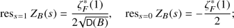
\(Z_B(s)\) has meromorphic continuation to \(\mathbb C \). More precisely:
-
(i)
If F is a number field, then \(Z_B(s)\) is holomorphic away from \(s=0,1/2,1\) with simple poles at \(s=0,1\) and residues
moreover, \(Z_B(s)\) is holomorphic at \(s=1/2\) if and only if B is a division algebra.
-
(ii)
If F is a function field of a curve of genus g over \(\mathbb F _q\), then \(Z_B(s)\) is holomorphic away from \(q^s=q^{0},q^{1/2},q^1\), with simple poles at \(q^s=q^0,q^1\) and residues

moreover, \(Z_B(s)\) is holomorphic where \(q^s=q^{1/2}\) if and only if B is a division algebra.
-
(i)
-
(b)
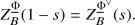
\(Z_B(s)\) satisfies a functional equation. More precisely:
-
(i)
If F is a number field, then

-
(ii)
If F is a function field, then

-
(i)


Proof. We apply Main Theorem 29.10.1 and Theorem 29.10.20 with \(\underline{\Phi }\) as in 29.8.9 with \(\Phi _v\) the characteristic function of a maximal order or the standard function according as v is nonarchimedean or archimedean, so \(\underline{\Phi }(0)=1\).
In the number field case, we have  self-dual when v is archimedean, and by (29.7.20) we have

and  when v is nonarchimedean. Multiplying these together and applying Theorem 29.10.1(c) gives

In the function field case, a similar argument holds but with the character modified by a global differential as in 29.8.9: for the relevant additional factor, see Exercise 29.13.
To conclude, we note that when \(B\simeq {{\,\mathrm{M}\,}}_2(F)\) then by Lemma 29.8.24 the nonarchimedean part of \(Z_B(s)\) is given by \(\zeta _F(2s)\zeta _F(2s-1)\), and this has a double pole at \(s=1/2\) (or accordingly \(q^{s-1/2}=1\)).□
Remark 29.10.24. In her 1929 Ph.D. thesis, Hey [Hey29] defined the zeta function of a division algebra over \(\mathbb Q \), proving that it has an Euler product and functional equation—this was a tour de force in algebraic and analytic number theory, especially at the time! For more on Hey’s contribution and its role in the development of class field theory, see the perspective by Roquette [Roq2006, §9], including Zorn’s observation that the functional equation yields an analytic proof of the classification of division algebras. Hey’s thesis was never published (though the content appears in Deuring [Deu68, VII, §8]), and classical treatments of the zeta function for the most part gave way to the development of Chevalley’s adeles and ideles.
Tate’s thesis [Tate67] (from 1950, published in 1967) is usually given as the standard reference for the adelic recasting of zeta and L-functions of global fields as above: it gives the general definition of a zeta function associated to a local field, an integrable function, and a quasi-character [Tate67, §2]; see also the Bourbaki seminar by Weil [Weil66]. But already in 1946, Matchett (also a student of Emil Artin) wrote a Ph.D. thesis at Indiana University [Mat46] beginning the redevelopment of Hecke’s theory of zeta and L-functions in terms of adeles and ideles. At the time, Iwasawa also contributed to the development of the theory; see his more recently published letter to Dieudonné [Iwa92].
These results were generalized to central simple algebras over local fields by Godement [God58a, God58b], Fujisaki [Fuj58], and Weil [Weil82, Chapter III] (and again Weil [Weil74, Chapter XI]) in the same style as Iwasawa and Tate; and then they were further generalized (allowing representations) by Godement–Jacquet [GJ72], providing motivation for the Langlands program.
As an example of the generalizations indicated by Remark 29.10.24, we conclude with a slightly more general statement.
Theorem 29.10.25
Let F be a global field, let B be a central division algebra over F, let \(\underline{\Phi }\) be a Schwartz–Bruhat function on \(\underline{B}\), and let \(\underline{\chi }:\underline{B}^\times \rightarrow \mathbb C \) be a unitary character such that \(\underline{\chi }\) restricted to \(\underline{F}^\times \) is trivial. Define
Then the function \(L_B^{\underline{\Phi }}(s, \underline{\chi })\) is absolutely convergent for \({{\,\mathrm{Re}\,}}s>1\). If \(\underline{\chi }\) is nontrivial, then \(L_B^{\underline{\Phi }}(s,\underline{\chi })\) has holomorphic continuation to \(\mathbb C \) and satisfies the functional equation

Proof. Proven in the same way as Main Theorem 29.10.1, just keeping track of the character \(\underline{\chi }\). The (possible) residues at \(s=0,1\) (or more generally in the function field case \(q^s=q^0,q^1\)) are multiplied by
which is zero when \(\underline{\chi }\) is nontrivial by character theory and therefore the L-function is fact holomorphic at these points.□
11 Tamagawa numbers
Building on Main Theorem 29.10.1, in this section we compute the measure of certain quotients with respect to the normalized idelic measure above. Let B be a quaternion algebra over the global field F.
Lemma 29.11.1
Let \(\Omega \) be the set of real ramified places in B, and let

Then the sequence
is exact, giving a compatible measure on \(\underline{B}^1\) denoted \(\tau ^1\). Under this measure, we have
Proof. The surjectivity of the reduced norm is locally established, and its kernel is \(\underline{B}^1\) by definition. The image of \(B^\times \) under the reduced norm is \(F_{>_{\Omega } 0}^\times \) by the Hasse–Schilling theorem of norms (Main Theorem 14.7.4), with kernel \(B^1\). Moreover, the natural inclusion
is also surjective by weak approximation. Putting these together, we obtain (29.11.2), which we might be tempted to summarize in the exact sequence of pointed sets
but we will resist the temptation.□
We now prove the final result in this chapter.
Theorem 29.11.3
Let B be a quaternion algebra over a global field F. Then
and
Proof. The equality \(\underline{\tau }^{(1)}(F^\times \backslash \underline{F}^{(1)})=\zeta _F^*(1)\) is the statement of Main Theorem 29.10.1(c) applied to \(B=F\). Then B is a division algebra, the equality \(\underline{\tau }^{(1)}(B^\times \backslash \underline{B}^{(1)})=\zeta _F^*(1)\) is again Main Theorem 29.10.1(c), and the equality \(\underline{\tau }^1(B^1 \backslash \underline{B}^1) = 1\) then follows from (29.11.2).
To conclude, we make the appropriate modifications in the remaining case, and suppose that \(B={{\,\mathrm{M}\,}}_2(F)\). Then \(B^1={{\,\mathrm{SL}\,}}_2(F)\) and similarly \(\underline{B}^1={{\,\mathrm{SL}\,}}_2(\underline{F})\). By the exact sequence (29.11.2), we may show \(\tau ^1({{\,\mathrm{SL}\,}}_2(F)\backslash {{\,\mathrm{SL}\,}}_2(\underline{F}))=\tau ^1({{\,\mathrm{SL}\,}}_2(\underline{F})/{{\,\mathrm{SL}\,}}_2(F))=1\).
We will do Fourier analysis on \(\underline{F}^2\), extended from \(\underline{F}\), with self-dual measure \(\underline{\tau }\) and character \(\psi \). Let \(\underline{\Phi }\) be a Schwartz function on \(\underline{F}^2\). The Fourier transform is

and Poisson summation reads

The group \({{\,\mathrm{SL}\,}}_2(\underline{F})\) acts on column vectors \(\underline{F}^2 \smallsetminus \{0\}\) by left multiplication, with the stabilizer of \(F^2 \smallsetminus \{0\}\) given by \({{\,\mathrm{SL}\,}}_2(F)\). Thus

From (29.11.4), we derive

and \(\left\| {\underline{\alpha }}\right\| _{{{\,\mathrm{SL}\,}}_2(\underline{F})}=1\). Plugging in (29.11.6) into (29.11.5), we have

Replacing  and \(\alpha \leftarrow (\alpha ^{\textsf {t} })^{-1}\) (preserving the measure) in (29.11.7) gives

Subtracting (29.11.8) from (29.11.5) gives

choosing \(\underline{\Phi }\) such that  , we obtain \(\underline{\tau }^1({{\,\mathrm{SL}\,}}_2(\underline{F})/{{\,\mathrm{SL}\,}}_2(F))=1\).□
Remark 29.11.9. We return to Remark 29.8.8. In general, there is a natural, intrinsic measure on the adelic points of a semisimple algebraic group \(\mathsf {G}\) over a number field F, called the Tamagawa measure. With respect to the Tamagawa measure, the volume \({{\,\mathrm{vol}\,}}(\mathsf {G}(\underline{F})/\mathsf {G}(F))\) is finite, and the Tamagawa number of \(\mathsf {G}\) (over F) is defined as
For example, in the above we computed the volume for the group \(\mathsf {G}\) associated to the group \(B^1\) of quaternions of reduced norm 1.
In the late 1950s, Tamagawa defined the Tamagawa measure [Tam66]. Weil [Weil82] (based on notes from lectures at Princeton 1959–1960), computed that \(\tau (G)=1\) for G a classical semisimple and simply connected group; the conjecture that this holds in general was known as Weil’s conjecture on Tamagawa numbers. This difficult conjecture was proven by the efforts of many people: see Scharlau [Scha2009, §2] for a history. In particular, the calculation of the Tamagawa number of the orthogonal group of a quadratic form recovers the Smith–Minkowski–Siegel mass formula that computes the mass of a genus of lattice.
Exercises
- 1.:
-
Let \(\mu _p\) be the standard Haar measure on \(\mathbb Q _p\).
- (a):
-
Let \(D(a,\delta ) :=\{x \in \mathbb Q _p : |x-a \,| < \delta \}\) be the open ball of radius \(\delta \in \mathbb R _{>0}\) around \(a \in \mathbb Q _p\). Compute the measure \(\mu _p(D(a,\delta ))\), and repeat with the closed ball of radius \(\delta \in \mathbb R _{\ge 0}\).
- (b):
-
Show that
$$\begin{aligned} \int _\mathbb{Z _p} \log (|x \,|_p)\,\mathrm{d }\mu _p(x) = -\frac{\log p}{p-1}. \end{aligned}$$
- 2.:
-
Let \(F :=\mathbb F _q(T)\); then F is the function field of \(\mathbb P ^1\), a curve of genus \(g=0\) and
$$\begin{aligned} \zeta _F(s) = \frac{1}{(1-q^{-s})(1-q^{1-s})}. \end{aligned}$$Let \(B :={{\,\mathrm{M}\,}}_2(F)\). Verify directly that \(\zeta _B(s)\) as defined in (29.8.1) satisfies \(\zeta _B(1-s)=q^{4-8s}\zeta _B(s)\), and then compare this with Theorem 29.10.23.
- 3.:
-
Let G be a locally compact, second countable topological group, and let \(H \le G\) be a subgroup.
- (a):
-
Show that G/H is locally compact. [Hint: Use Exercise 12.4.]
- (b):
-
If H is closed, show that G/H is Hausdorff (repeating Exercise 12.5).
[We do not need G to be Hausdorff in this exercise.]
- 4.:
-
Let G be a Hausdorff, locally compact, second countable topological group.
- (a):
-
Let \(\mu ,\mu '\) be two Haar measures on G. Show that there exists \(\kappa \in \mathbb R _{>0}\) such that \(\mu '=\kappa \mu \).
- (b):
-
Let \(\mu \) be a left Haar measure on G. Show that \(\mu (G)<\infty \) if and only if G is compact. [Hint: Use Exercise 12.4.]
 5.:
5.:-
Let G be a Hausdorff, locally compact, second countable topological group. Let \(\mu \) be a left Haar measure on G. Show that the modular function \(\Delta _G:G \rightarrow \mathbb R _{>0}\) is a homomorphism of groups.
 6.:
6.:-
Let A be a Hausdorff, locally compact, second countable topological ring, and let \(a,b \in A^\times \). Show that
$$\begin{aligned} \left\| {ab}\right\| =\left\| {a}\right\| \left\| {b}\right\| . \end{aligned}$$ - 7.:
-
Consider the exact sequences
$$\begin{aligned} 1 \rightarrow \{\pm 1\} \rightarrow \mathbb R ^\times \xrightarrow {\phi } \mathbb R ^\times _{>0} \rightarrow 1 \end{aligned}$$where the map \(\phi \) is given by either the quotient by \(\pm 1\) (equivalently, the absolute value) or by the map \(x \mapsto x^2\). Equip \(\mathbb R ^\times \) and \(\mathbb R ^\times _{>0}\) with the standard Haar measure \(\mathrm{d }{x}/|x \,|\). Compute the unique compatible measures on \(\{\pm 1\}\) for the two choices of \(\phi \) and show they differ by a factor 2.
- 8.:
-
Finish the proof of Lemma 29.5.18. [Hint: It may help to use the Iwasawa decomposition (Proposition 33.4.2 and Lemma 36.2.7).]
 9.:
9.:-
Prove Proposition 29.6.9, as follows. Let F be a nonarchimedean local field and let \(\psi :F \rightarrow \mathbb C ^1\) be a nontrivial unitary character of F, for example the standard unitary character. For each \(x \in F\), let \(\psi _x :F \rightarrow \mathbb C ^1\) be defined by \(\psi _x(y)=\psi (xy)\).
- (a):
-
Show that \(\psi _x\) is again a unitary character of F and that \(\psi _x\) is trivial if and only if \(x=0\).
- (b):
-
Show that

defines a continuous, injective group homomorphism. [Hint: recall that
 inherits a compact-open topology, so a basis of neighborhoods of the identity is given by
  for \(K \subseteq F\) compact and
  an open neighborhood of 1. Given such K, V, show that there exists an open neighborhood \(U \subseteq F\) of 0 such that \(xK \subseteq \psi ^{-1} V\) for all \(x \in U\).]
 - (c):
-
Show that \(\Psi (F)\) is dense in
 . [Hint: if \(\psi _x(y)=0\) for all \(x \in F\), then \(y=0\).]
 - (d):
-
Prove that \(\Psi ^{-1}\) is continuous (on its image). [Hint: work in the other direction in (b).]
- (e):
-
Show that \(\Psi (F)\) is complete, hence closed, subgroup of
 . Conclude that \(\Psi \) is an isomorphism of topological groups.
 10.:
10.:-
Complete the proof of Theorem 29.10.20 for F a number field, as follows. By choice of \(B'\), we showed that \(Z_B^{\Phi }(s)\) is holomorphic except for \(s=0,1\) and possibly when \(q_v^s=q_v^{1/2}\) for \(v \in {{\,\mathrm{Ram}\,}}(B')\). Show (by varying the choice of \(B'\)) that \(Z_B^{\Phi }(s)\) is holomorphic away from \(s=0,1/2,1\).
 11.:
11.:-
Let B be a quaternion algebra over a global field F. Show that there exists a compact
 such that the map \(\underline{B}\rightarrow B\backslash \underline{B}\) is not injective on
  . [Hint: accept the results of section 29.3 and take
  with measure
  and integrate.]
 - 12.:
-
Following the proof of Theorem 29.11.3, show that if \(B={{\,\mathrm{M}\,}}_n(F)\) that
$$\begin{aligned} \underline{\tau }^{(1)}(B^\times \backslash \underline{B}^{(1)})=\underline{\tau }^{(1)}(F^\times \backslash \underline{F}^{(1)})=\zeta _F^*(1) \end{aligned}$$and
$$ \underline{\tau }^1(B^1 \backslash \underline{B}^1) = 1. $$ - 13.:
-
This exercise assumes some background in algebraic curves, see e.g. Silverman [Sil2009, Chapter II]—for a wider survey, see Rosen [Ros2002]. Let F be the function field of a curve X over \(\mathbb F _q\). Thedivisor group \({{\,\mathrm{Div}\,}}X\) is the free abelian group on the set of places v; it has a degree map \(\deg :{{\,\mathrm{Div}\,}}X \rightarrow \mathbb Z \) with \(\deg v = [k_v:\mathbb F _q]\), where \(k_v\) is the residue field at v An element \(f \in F^\times \) has a divisor \({{\,\mathrm{div}\,}}f = \sum _v {{\,\mathrm{ord}\,}}_v(f) v\). A nonzero meromorphic differential \(\omega \) on X has also a divisor \(K :=\sum _v a_v v\) where \(a_v={{\,\mathrm{ord}\,}}_v(\omega /\mathrm{d }{t}_v)\) where \(t_v\) is a uniformizer at v; we call K acanonical divisor. Given \(D=\sum _v d_v v \in {{\,\mathrm{Div}\,}}X\), let
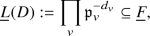
and
 and finally \(\ell (D) :=\dim _\mathbb{F _q} L(D)\). Define thegenus of X or of F by \(g :=\ell (K) \in \mathbb Z _{\ge 0}\).
 - (a):
-
Show that the characteristic function \(\underline{\Phi }\) of
 is \(q^{\deg D - \deg K/2}\) times the characteristic function of
  .
. - (b):
-
Apply Poisson summation to \(\underline{\Phi }\) to obtain
$$\begin{aligned} \sum _{f \in L(D)} 1&= q^{\deg D - \deg K/2} \sum _{f \in L(K-D)} 1 \\ \ell (D)&= \deg D - \frac{1}{2}\deg K + \ell (K-D). \end{aligned}$$ - (c):
-
Plug in \(D=0\) to (b) to get \(L(0)=\mathbb F _q\) the constant functions and conclude \(\deg K = 2g-2\).
- (d):
-
Conclude theRiemann–Roch theorem
$$\begin{aligned} \ell (D)-\ell (K-D) = \deg D + 1 -g. \end{aligned}$$(29.11.10)
- 14.:
-
Prove Theorem 29.10.25.
 5.:
5.: 6.:
6.: 9.:
9.:
 inherits a compact-open topology, so a basis of neighborhoods of the identity is given by
  for
for  an open neighborhood of 1. Given such K, V, show that there exists an open neighborhood
  . [Hint: if
  . Conclude that
  10.:
10.: 11.:
11.: such that the map
  . [Hint: accept the results of section
  with measure
  and integrate.]
 and finally
  is
is  .
.Author information
Authors and Affiliations
Corresponding author
Rights and permissions
This chapter is distributed under the terms of the Creative Commons Attribution 4.0 International License (http://creativecommons.org/licenses/by/4.0/), which permits use, duplication, adaptation, distribution and reproduction in any medium or format, as long as you give appropriate credit to the original author(s) and the source, a link is provided to the Creative Commons license and any changes made are indicated.The images or other third party material in this chapter are included in the work's Creative Commons license, unless indicated otherwise in the credit line; if such material is not included in the work's Creative Commons license and the respective action is not permitted by statutory regulation, users will need to obtain permission from the license holder to duplicate, adapt or reproduce the material.
Copyright information
© 2021 The Author(s)
About this chapter

Cite this chapter
Voight, J. (2021). Idelic zeta functions. In: Quaternion Algebras. Graduate Texts in Mathematics, vol 288. Springer, Cham. https://doi.org/10.1007/978-3-030-56694-4_29
Download citation
DOI: https://doi.org/10.1007/978-3-030-56694-4_29
Published:
Publisher Name: Springer, Cham
Print ISBN: 978-3-030-56692-0
Online ISBN: 978-3-030-56694-4
eBook Packages: Mathematics and StatisticsMathematics and Statistics (R0)