Biomedical Signal Processing: An ECG Application

Abstract

The electrocardiogram (ECG) is a low-cost non-invasive sensor that measures conduction through the heart. By interpreting the morphology of a person’s ECG, clinical domain experts are able to infer the functionality of the underlying heartbeat, and diagnose irregularities. Moreover, a variety of signal processing algorithms have been developed to automatically monitor ECG recordings for patients and clinicians, both in and out of the clinical setting. The periodic nature of the ECG makes it particularly suitable for frequency-based analysis. Wavelet analysis, which uses brief oscillators to extract information from different portions of the signals, has proven highly effective. This chapter demonstrates the application of the continuous wavelet transform on multi-channel ECG signals from patients with arrhythmias. The information extracted is used to develop a high-performing heartbeat classifier that can distinguish between various types of regular and irregular beats.

FormalPara Learning Objectives

• Understand the principles of electrocardiography.

• Understand signals in the time and frequency domain.

• Learn the importance of applying linear filters to clean signals.

• Understand wavelet analysis, a traditional signal processing technique, and apply it to the electrocardiogram (ECG).

This workshop introduces the concepts and workings of the ECG, and signal processing techniques used to glean information from raw recordings. In the hands-on coding exercises, you will be asked to apply the signal processing methods on a clinical prediction problem.

1 Requirements

• Linear algebra.

• Understanding of basic concepts of electrical conduction.

• Programming in Python.

• Understanding of supervised classification (see Chap. 2.06).

2 Physiologic Signal Processing

2.1 Introduction

A signal conveys information about the underlying system being measured. There are many techniques used to measure time-varying biosignals from human bodies. Examples of invasive signals collected include: intra-arterial blood pressure and cell membrane potential measurements. Much more prevalent however, are non-invasive signals, most of which are bioelectrical, including the electrocardiogram, and electroencephalogram.

Clinical domain experts are able to interpret the signal shapes, or waveforms, to extract insights. For example, the non-compliant vessels of a patient with stiff arteries may produce a reflected pressure wave in response to systolic pressure (Mills et al. 2008). By examining the patient’s arterial blood pressure waveform, a clinician may observe a notch followed by a delayed rise, where they would normally expect the systolic upstroke to end, and therefore diagnose the arterial stiffness.

For the past several decades however, automated algorithms have been developed to detect notable events and diagnose conditions. Although domain experts are usually required to create and validate these algorithms, once they are developed and implemented, they are able to automate tasks and free up human labor. A prominent example is the use of built-in arrhythmia alarms in bedside monitors that record ECGs. Instead of requiring a clinician to constantly monitor a patient’s waveforms, the machine will sound an alarm to alert the medical worker, only if an anomaly is detected. The hospital bedside is far from the only place where biosignals can be utilized. Due to the low-cost and portability of sensors and microprocessors, physiologic signals can be effectively measured and analyzed in almost any living situation, including in remote low-resource settings for global health.

Traditional signal processing techniques have proven very effective in extracting information from signal morphology. This chapter will describe the principles of the ECG, and explore interpretable techniques applied on a relevant clinical problem: the classification of heart beats.

2.2 The Electrocardiogram

This section provides a simple overview of the ECG to support the signal processing in the rest of the chapter. For an in-depth description of action potentials and the ECG, see (Venegas and Mark 2004).

The electrocardiogram (ECG) is a non-invasive time-varying voltage recording used by physicians to inspect the functionality of hearts. The potential difference between a set of electrodes attached to different parts of the body’s surface, shows the electrical activity of the heart throughout the cardiac cycle.

2.2.1 Action Potentials and the Cardiac Cycle

The cardiac cycle consists of two phases: diastole, during which the heart muscle (myocardium) relaxes and fills with blood, followed by systole, during which the heart muscle contracts and pumps blood. The mechanism that actually triggers individual muscle cells to contract is the action potential, where the membrane potential of a cell, its potential relative to the surrounding extracellular fluid, rapidly rises and falls. Na+, Ca2+, and K+ ions flow in and out of the cell, depolarizing and then repolarizing is membrane potential from its negative resting point.

On a larger scale, each action potential can trigger an action potential in adjacent excitable cells, thereby creating a propagating wave of depolarization and repolarization across the myocardium. During a healthy heartbeat, the depolarization originates in pacemaker cells which ‘set the pace’, located in the heart’s sinoatrial (SA) node. This then spreads throughout the atrium, the atrioventricular (AV) node, the bundles of His, the Purkinje fibers, and finally throughout the ventricles (Fig. 17.1).

Fig. 17.1

Conduction pathways of the heart and corresponding membrane potentials (Venegas and Mark 2004)

2.2.2 Electrocardiogram Leads

The electrical activity of the myocardium produces currents that flow within the body, resulting in potential differences across the surface of the skin that can be measured. Electrodes are conductive pads attached to the skin surface. A pair of electrodes that measure the potential difference between their attachment points, forms a lead. A wave of depolarization traveling towards a lead produces a positive deflection, and vice versa.

The magnitude and direction of reflection measured by a lead depends on the axis that it measures. By combining multiple leads, a more complete picture of the heart’s 3-dimensional conduction can be viewed across multiple axes. The standard 12-lead ECG system is arranged as follows:

• 1. Limb Leads—I, II, III. Three electrodes are placed on the limbs: left arm (LA), right arm (RA), and left leg (LL). These electrodes then form leads I = LA–RA, II = LL–RA, and III = LL–LA. The virtual electrode Wilson’s Central Terminal is the average of the measurements from each limb electrode.

• 2. Augmented limb leads—aVR, aVL, and aVF. These are derived from the same electrodes as used in the limb leads, and can be calculated from the limb leads. The limb leads and augmented limb leads provide a view of the frontal plane of the heart’s electrical activity.

• 3. Precordial leads—V1, V2, V3, V4, V5, V6. These leads measure the electrical activity in the transverse plane. Each lead measures the potential difference between an electrode placed on the torso, and Wilson’s Central Terminal (Figs. 17.2, 17.3 and 17.4).

  Fig. 17.2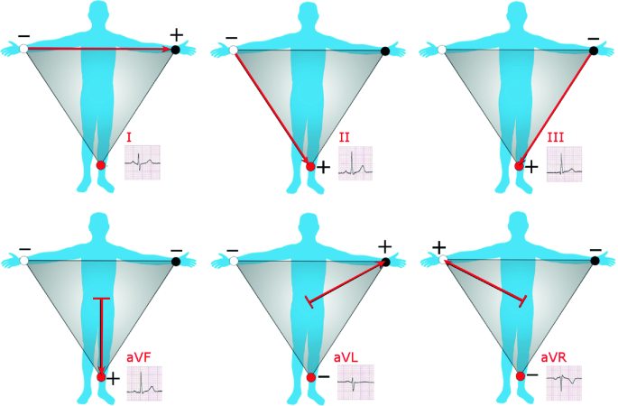

  

  Frontal leads of the ECG (Npatchett 2020)

  Fig. 17.3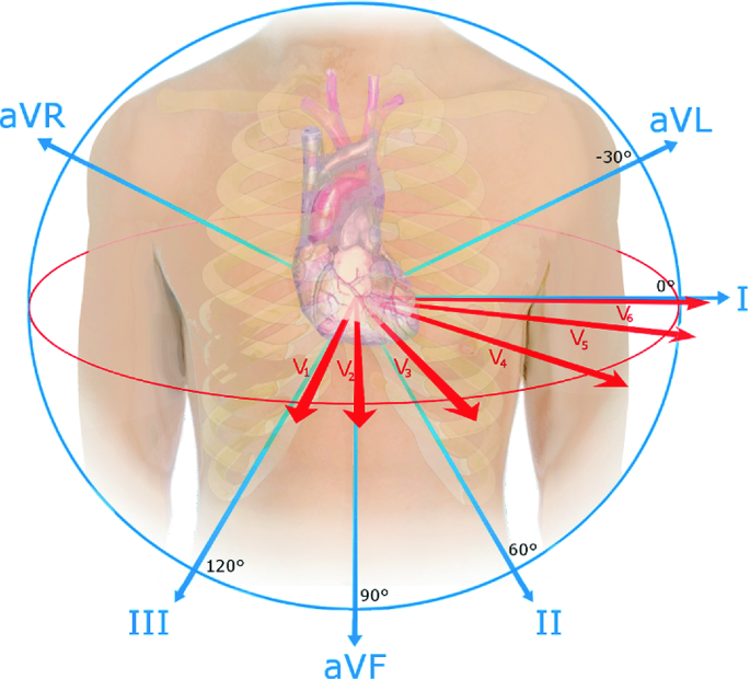

  

  Precordial leads of the ECG (File:EKG leads.png 2016)

  Fig. 17.4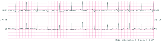

  

  Two channel ECG recording of normal sinus rhythm

Expert clinicians are able to use different leads to more effectively diagnose different conditions. An arrhythmia that disrupts the regular conduction perpendicular to the axis of a lead may not show up at all in the ECG lead, if all appears normal in the direction of axis.

But although having 12 leads provides a rich view of the heart, even a single lead may provide plenty of information depending on the problem at hand. In addition, requiring the placement of too many electrodes may be cumbersome and impractical in a remote setting. In this chapter and its practical exercises, we will use leads MLII (a modified lead II) and V5, due to the availability of data. One limb and one precordial lead provides plenty of information for the developed beat classification algorithms.

2.2.3 Interpretation of the Electrocardiogram

Figure 17.5 shows a model lead II recording of a normal beat. Recall that depolarization towards the positive electrode (LA) produces a positive deflection. The segments of the ECG can be broken down as follows (Fig. 17.6):

Fig. 17.5

Lead II ECG recording (File:SinusRhythmLabels.svg 2019)

Fig. 17.6

Cardiac cycle (File:2027 Phases of the Cardiac Cycle.jpg 2017)

• The P wave represents atrial depolarization. Atrial systole begins after the P-wave onset, lasts about 100 ms, and completes before ventricular systole begins.

• The QRS complex represents ventricular depolarization. The ventricular walls have more mass and are thicker than the atrial walls. This, along with the angle and conduction flow of the ventricles relative to lead II, makes the QRS complex the most prominent feature shown in this ECG, and the target of most beat detectors. Atrial repolarization also occurs during this time, but is obscured by the large signal. Ventricular systole begins towards the end of the QRS complex.

• The T wave represents ventricular repolarization, and marks the beginning of ventricular diastole.

An ECG can convey a large amount of information about the structure of the heart and the function of its underlying conduction system, including: the rate and rhythm of heartbeats, the size and position of the chambers, and the presence of damage to the myocytes or conduction system.

2.2.4 Normal Beats and Arrhythmias

One of the most useful functionalities of the ECG is its use in monitoring healthy heartbeats and diagnosing arrhythmias. This chapter will focus on identifying four types of beats in particular:

• Normal—The conduction originates in the sinoatrial node, and spreads throughout the atrium, passes through the atrioventricular node down into the bundle of His and into the Purkinje fibers, spreading down and to the left throughout the ventricles. The left and right ventricles contract and depolarize almost simultaneously.

• Left bundle branch block (LBBB)—The left bundle is blocked, while the impulses continue to conduct through the right bundle and depolarize the right ventricle. This initial wave spreads towards lead V1, producing a small positive deflection. Soon after, depolarization spreads from the right ventricle to the left, away from V1, because the left ventricle has more mass than the right, the overall deflection is still negative. The delayed left ventricular contraction results in a wider QRS complex.

• Right bundle branch block (RBBB)—The right bundle is blocked. Depolarization spreads from the left bundle through the left ventricle away from lead V1, producing a negative deflection in V1. After a delay, the depolarization spreads from the left ventricle through the right towards V1, producing a positive deflection.

• Ventricular premature beat—An extra heartbeat originates from one of the ventricles, rather than the SA node. The ventricles are activated by an abnormal firing site, disrupting the regular rhythm. In channel II, this results in the lack of a p-wave, since the beat does not begin with atrial depolarization. Furthermore, the action potential spreads across the myocytes rather than directly through the conduction fibers, resulting in a wider QRS complex.

As a physician looks upon a visual ECG diagram and interprets the underlying workings or irregularities of the heart, so too can algorithms be developed to automatically process these signals and reveal arrhythmias (Fig. 17.7).

Fig. 17.7

Two channel ECG recordings of four beat types

2.2.5 ECG Databases

The data used in this chapter is from the MIT-BIH Arrhythmia Database https://physionet.org/physiobank/database/mitdb/, which contains 30 min ECG recordings of patients with a range of arrhythmias and normal beats. It is a landmark database, used as an FDA standard for testing automated arrhythmia detectors. Each recording has two channels, and a set of labelled beat annotations that will be used as the ground truth. Therefore, the tasks of obtaining and diagnosing the beats are already done, and the focus can be placed solely on developing the algorithms used to classify the beats into the correct groups.

2.3 Time and Frequency Information

The frequency domain allows the analysis of the signal with respect to frequency, as opposed to the commonly used time domain. We can not only observe how a signal changes over time, but also how much of the signal’s energy lies within each frequency band.

2.3.1 ECG Frequency Information

Frequency analysis is very naturally applied to ECGs, which can be modelled as a sum of oscillators, due to their periodic nature. Most of the clinically relevant energy in a QRS complex has been found to lie within 4 and 30 Hz. Regarding the entire heartbeat, a very slow heart rate of 30 beat per minute (bpm), which lies on the lower end of realistically occurring heart rates, corresponds to 0.5 Hz. The upper bound heart rate (around 200 bpm) will always be of a lower frequency than the components of an individual QRS complex.

In addition to the signal produced by the heart beats themselves which are of interest, there are several prominent sources of noise which should be removed: baseline wander, power line interference, and muscle noise. Baseline wander is generally low frequency offsets or oscillations due to slow movement that moves the electrodes, such as breathing. Power lines of 50 Hz or 60 Hz depending on the country, create sinusoidal electromagnetic fields which can be detected by the ECG. Finally, action potentials caused by muscles other than the heart propagate through the body. They exhibit a wide range of frequencies that overlaps with that of the ECG, and are highly variable.

When filtering, the goal is to filter away the noise without also removing the relevant information. Therefore, given all the above information, when filtering ECGs to remove unwanted energy components, a commonly chosen bandpass range is 0.5–40 Hz. A narrow bandstop filter centered about the power line frequency may also be applied. It is more difficult to remove muscle noise due to it not being characterized by fixed frequency ranges or power ratios, though when movement is minimized, the effects of this noise are rather low. One method is to build an adaptive filter, using a known clean ECG as a reference, though this will not be covered in this chapter.

2.3.2 The Fourier Transform

The Fourier transform is an operation that converts a function of time into a sum of sinusoids, each of which represent a frequency component in the resultant frequency domain (Freeman 2011). The discrete Fourier transform, applied to sampled digital signals, is a linear transform and also the primary function used for frequency analysis.

It characterizes a periodic signal more accurately when applied to more complete cycles. Therefore, it would be more effective when applied to a long series of similar ECG beats. But for the task of beat classification, each beat must be observed and treated in isolation, as irregular beats can suddenly manifest and disappear. If we take a long segment of tens of uniform ECG beats and single differing beat, and inspect the frequency content of the entire segment, the anomalous beat’s frequency information would be drowned out by the energy of the more common beats.

With the Fourier transform, there is a direct tradeoff between more accurately characterizing the frequency information with a longer signal, and isolating beats with a shorter signal. Another very effective technique for the frequency analysis of individual beats, is wavelet analysis.

2.4 Wavelets

A wavelet is a time localized oscillation, with an amplitude that begins at zero, rises, and decreases back to zero (Mallat 2009). They can be used to extract information from data such as audio signals, images, and physiologic waveforms. Wavelets are defined by a wavelet function ψ(t) shown in Eq. 17.1, which can also be called the ‘mother wavelet’. There are many wavelet functions such as the Ricker wavelet and the Morlet wavelet, which are generally crafted to have specific properties to be used for signal processing.

A mother wavelet may be scaled by factor a and translated by factor b to produce a series of child wavelets. Increasing the scale factor stretches the wavelet to make it less localized in time, allowing it to correlate with lower frequency signals, and vice versa.

$$\psi_{a,b} (t) - \frac{1}{\sqrt a } \psi \left( {\frac{t - b}{a}} \right)\,\,(Wavelet\,series\,equation)$$

(17.1)

$$X_{w} (a ,b) = \frac{1}{{\left| a \right|^{1/2} }}\int_{ - \infty }^{\infty } {x(t)\overline{\psi } } \left( {\frac{t - b}{a}} \right)dt\,\,(Continuous\,wavelet\,transform)$$

(17.2)

Equation 17.2 shows the formula for the continuous wavelet transform (CWT) of a signal x(t), where the signal is convolved with the complex conjugate of a wavelet of a certain scale. The convolution operation between signal 1 and signal 2 can be thought of as sliding signal 1 from one edge of signal 2 to the other, and taking the sum of the multiplication of the overlapping signals at each point. As each wavelet is convolved with the input signal, if the signal segment is of a similar shape to the wavelet, the output of the wavelet transform will be large. Therefore, applying the CWT using a range of scale factors, allows the extraction of information from the target signal at a range of frequencies (Fig. 17.8).

Fig. 17.8

Child wavelets of different scale values

A key advantage of the CWT for frequency analysis is its ability to isolate information from a signal in both frequency and time, due to the variable scale and shift factors. For example, applying a compressed wavelet with a low scale factor may detect high frequency components in the QRS complex of the ECG, but not in the flatline period between the T and P waves.

2.5 Classifying Beats with Wavelets

There are several steps in using wavelets for the beat classification task:

• 1. Apply the CWT to the ECG beats.

• 2. Derive features from the output of the CWT.

• 3. Feed these final features into a supervised classifier.

2.5.1 Applying the Continuous Wavelet Transform

The CWT requires two parameters that must be chosen: the wavelet function(s), and the scale factor(s). Observing the two channels for the various beat types, it can be seen that there are two general shapes of the QRS complexes: single spike, and sinusoid. Therefore, it will be effective to choose one wavelet shaped like each QRS complex type, so that the convolution results will detect which of the two shapes each waveform is more similar to. For example, we can choose the ‘gaus1’ wavelet shown below to accentuate the sinusoid QRS complexes, and the ‘gaus2’ wavelet to accentuate the sharp spike complexes. There are many wavelet families and functions to choose from, and the functions can even be considered a hyperparameter to optimize for beat discrimination; using the two below for the aforementioned reasons is a good starting point (Fig. 17.9).

Fig. 17.9

Two wavelet functions from the Gaussian wavelet family. Generated using (Lee et al. 2019) 

Next, the wavelet scales must be appropriately set to capture the correct frequency information. As previously stated, the frequencies of interest in the ECG are between 0.5 and 40 Hz, there. A larger scale wavelet will pick up a wider complex, which will be useful for example, in differentiating channel V1 of LBBB and normal beats. For a given mother wavelet, each child wavelet of a certain scale has a corresponding center frequency that captures the frequency of its most prominent component. The range of scales can be chosen to cover the range of ECG frequencies. Once again, the more scales used, the more features and potential sources of noise generated.

If the data is available, using two simultaneous ECG channels can be much more effective than using just a single lead. Each channel provides a different viewpoint of the electrical conduction of the heart, and both clinicians and algorithms can make a more accurate diagnosis when combining multiple sources of information to generate a more complete picture. In some instances, the difference between beat types is not as obvious in a single lead. For instance, the difference between RBBB and ventricular premature beat is more obvious in lead MLII, but less so in lead V1. Conversely, the difference between RBBB and LBBB is more obvious in lead V1 than in lead MLII. When limited to a single lead, the algorithm or clinician has to be able to pick up more subtle differences.

Figure 17.10 shows the CWT applied to each lead of a normal beat, using the two wavelet functions, at various scales. The heatmap of gaus2 applied to signal MLII is the highest (more red) when the single spike QRS complex aligns with the symmetrical wavelet of a similar width. Conversely, the heat-map of gaus2 applied to signal V1 is the lowest when (more blue) when the downward QRS aligns with the wavelet to produce a large negative overlap.

Fig. 17.10

Two channel ECG of normal beat and output of applied CWT

2.5.2 Deriving Features from the CWT

For each beat, we will have a CWT matrix for each channel (c) and wavelet function (w). For instance, 2 × 2 = 4. Each CWT matrix has size equal to the number of scales (s) multiplied by the length of the beat (l). For instance, 5 × 240 = 1200. In total this gives around 4800 data points, which is more than the original number of samples in the beat itself, whereas the goal of this signal processing is to extract information from the raw samples to produce fewer features.

As a general rule of thumb, the number of features should never be on the same order of magnitude as the number of data points. With the MITDB dataset, there are several thousand of each beat type, so the number of features must be lower than this.

Although the CWT has produced more data points, it has transformed the input data into a form in which the same type of time and frequency information can be extracted using a consistent technique. This would not be possible with the raw ECGs in their time domain representation. One such technique may be to take the maximum and minimum value of the CWT, and their respective sample indices, for each scale. The min/max values of the dot products indicate how strongly the wavelet shapes match the most prominent ECG waveform sections, and their indices give insight regarding the distribution and location of the QRS complexes. In RBBB beats for instance, the maximum overlap index of the ‘gaus1’ wavelet with signal MLII tends to occur later than that of the ‘gaus2’ wavelet with the same signal. This divides the number of data points by the number of samples, and multiplies it by 4, giving 4800 × 4/240 = 80 features, which is more reasonable. This pooling method only draws a fixed amount of information from each wavelet scale, and loses other potential data such as the T wave morphology. However, it is simple to implement and already very effective in discriminating the different beat types (Fig. 17.11).

Fig. 17.11

Two channel ECG of RBBB beat and output of applied CWT

Although feature engineering and parameter tuning is required, these fundamental signal processing techniques offer full transparency and interpretability, which is important in the medical setting. In addition, the algorithms are relatively inexpensive to compute, and simple to implement, making them highly applicable to remote monitoring applications.

2.5.3 Using CWT Features to Perform Classification

See Chap. 12 for the background description of supervised classification in machine learning.

Once the features have been extracted from the CWT matrices for each labeled beat, the task is reduced to a straightforward supervised classification problem. Most of the algorithmic novelty is already applied in the signal processing section before actually reaching this point, which is the starting point for many machine-learning problems.

In this dataset, there are no missing values to impute as the CWT is able to be applied to each complete beat. However, it is very common to have missing or invalid samples when measuring ECGs, due to factors such as detached electrodes or limbs touching. Usually the raw waveforms themselves are cleaned, selectively segmented, and/or imputed, rather than the features derived from them.

Each feature should be normalized between a fixed range such as 0–1, in order to equally weight the variation in each dimension when applying the classifier. The features can be fed through a supervised classifier, such as a logistic regression classifier, k-nearest neighbors classifier, support vector machine, or feed-forward neural network. As usual, the data should be split into a training and testing set, or multiple sets for k-fold cross-validation. Once the classifiers are trained, they can be used to evaluate any new beats.

The results of the classifier can be shown by a confusion matrix, whose two axes represent instances of the predicted class, and instances of the actual class. The matrix contains the number of true positives (TP), true negative (TN), false positive (FP), and false negative (FN) values for each class. Using these values, performance metrics can be calculated (Tables 17.1 and 17.2):

Table 17.1 Example confusion matrix for beat classification

Table 17.2 Performance metrics calculated from confusion matrix in Table 17.1

In binary classification tasks, a receiver operating characteristic curve (ROC), which plots the true positive rate against the false positive rate, can be generated from a classifier by sweeping the discrimination threshold used to make the final classification. The area under the ROC (AUROC) can then be calculated to provide a single measurement of performance. But it is not as straightforward to create a ROC for multi-class classification when there are more than two classes, as there is no single threshold that can be used to separate all classes. One possible alternative is to binarize the labels as ‘this’ or ‘other’, test the classifier, and generate the ROC for each class. Following this, an average of all the AUROCs could be calculated. However, retraining the classifier by relabeling the data will produce different decision boundaries, and hence neither of the individual re-trained classifiers could reliably be said to represent the true performance of the original multi-class classifier. It is usually sufficient to provide the precision, recall, and f1-score.

3 Exercises

The exercises are located in the code repository: https://github.com/cx1111/beat-classifier.

The analysis subdirectory contains the following Jupyter notebook files:

• 0-explore.ipynb—exploration and visualization of the database, different ECG beats, and applying filtering.

• 1-wavelets.ipynb—inspecting wavelet functions, matching wavelets to ECG morphologies, applying the CWT and using derived features for beat classification.

4 Uses and Limitations

Both inpatient and outpatient services in the hospital make use of waveforms, such as using blood pressure cuffs in routine checkups. In particular, intensive care unit (ICU) patients frequently have their respiratory and circulatory systems monitored with ECGs, photoplethysmograms, and more. The monitoring devices often have in-built algorithms and alarm systems to detect and alert clinicians of potentially dangerous artefacts such as arrhythmias.

The hospital bedside is far from the only place where biosignals can be utilized. Several factors drive the ubiquitous usage of physiologic signals in the modern global health domain:

• The low cost of instruments. The circuits, microprocessors, wires, and electrodes needed to measure simple potentials on the surface of a person’s skin, are all manufactured at scale at a low price. These cheap microprocessors are also sufficiently powerful to implement most ECG processing algorithms in real time, given the common sampling frequency of 125 Hz. The set of instruments can be bought for tens of dollars or less.

• The non-invasive portable nature of the technology. An ECG device for example, requires a microprocessor that can fit in a hand, along with a few cables and coin sized electrodes. Even certain smartwatches such as the Apple Watch, and the Fitbit, have the ability to measure, stream, and upload waveforms from their wearers. The mobility and simplicity of a technology which only requires a person to stick some electrodes on their skin, or wear a watch, allows it to be used in almost any setting.

• As previously mentioned, once algorithms are validated, they automate services that would normally be required from human experts. They can be especially effective in low income and remote areas with a scarcity of health workers. And even without automated algorithms, the prevalence of telemedicine allows remote health workers to visually inspect the easily measured waveforms.

The perpetual physiologic monitoring of people from richer countries via their mobile devices, along with the increasing accessibility of these technologies for people from low resourced countries, presents the unprecedented opportunity to learn from vast amounts of physiologic data. As the volume of physiologic signals collected across the globe continues to explode, so too will the utility of signal processing techniques applied to them.

But despite the popularity of this field, most clinical problems are not perfectly solved. The single aspect that makes signal processing both effective and challenging is the unstructured time-series data. Clearly the large number of samples contain actionable information, but the building of structured features from this data can seem almost unbound. Unlike a structured table of patient demographics and disease statuses for example, the raw samples of an arbitrary length signal are not immediately actionable. One would have to choose window lengths, the algorithm(s) to apply, the number of desired feature desired, and so forth, before having any actionable information.

A key challenge in developing the algorithms is the quality of the data collected. The algorithms developed in this chapter are applied to clean labelled signals, but this data is rarely available in practice. Among the most common indicators of poor-quality signals are missing samples due to instrumentation error or sensor misplacement/interference, and excessive noise from movement or other sources. An approach to building algorithms includes an initial step of only focusing on ‘valid’ sections, and tossing ‘invalid’ ones. But once again, the techniques used in this step must be validated, and the meaning of the labels themselves are somewhat subjective.

Finally, even when the performance of an algorithm is high, it is unlikely to be perfect. This requires decisions to be made to adjust tradeoffs between precision and recall, which in itself is difficult to objectively decide.

References

Resources
By Npatchett-Own work, CC BY-SA 4.0 (2020) https://commons.wikimedia.org/w/index.php?curid=39235282.
File:2027 Phases of the Cardiac Cycle.jpg. (2017). Wikimedia commons, the free media repository. Retrieved May 15, 2019, from https://commons.wikimedia.org/w/index.php?title=File:2027_Phases_of_the_Cardiac_Cycle.jpg&oldid=269849285.
File:EKG leads.png. (2016). Wikimedia commons, the free media repository. Retrieved May 15, 2019, from https://commons.wikimedia.org/w/index.php?title=File:EKG_leads.png&oldid=217149262.
File:SinusRhythmLabels.svg. (2019). Wikimedia commons, the free media repository. Retrieved May 15, 2019, from https://commons.wikimedia.org/w/index.php?title=File:SinusRhythmLabels.svg&oldid=343583368.
Freeman, D. (2011) 6.003 signals and systems. Massachusetts Institute of Technology, MIT OpenCourseWare. https://ocw.mit.edu.
Lee, G. et al. (2019). PyWavelets: A Python package for wavelet analysis. Journal of Open Source Software, 4(36), 1237. https://doi.org/10.21105/joss.01237
Mallat, S. (2009). A wavelet tour of signal processing: The sparse way (3rd ed.) Elsevier.
Mills, N. L. et al. (2008). Increased arterial stiffness in patients with chronic obstructive pulmonary disease: A mechanism for increased cardiovascular risk. Thorax, 63(4), 306–311.
Venegas, J., & Mark, R. (2004) HST.542 J quantitative physiology: Organ transport systems. Massachusetts Institute of Technology, MIT OpenCourseWare. https://ocw.mit.edu.
Author information
Authors and Affiliations
Corresponding author
Editor information
Editors and Affiliations
Rights and permissions
Open Access This chapter is licensed under the terms of the Creative Commons Attribution 4.0 International License (http://creativecommons.org/licenses/by/4.0/), which permits use, sharing, adaptation, distribution and reproduction in any medium or format, as long as you give appropriate credit to the original author(s) and the source, provide a link to the Creative Commons license and indicate if changes were made.
The images or other third party material in this chapter are included in the chapter's Creative Commons license, unless indicated otherwise in a credit line to the material. If material is not included in the chapter's Creative Commons license and your intended use is not permitted by statutory regulation or exceeds the permitted use, you will need to obtain permission directly from the copyright holder.
Copyright information
© 2020 The Author(s)
About this chapter
Cite this chapter
Xie, C. (2020). Biomedical Signal Processing: An ECG Application. In: Celi, L., Majumder, M., Ordóñez, P., Osorio, J., Paik, K., Somai, M. (eds) Leveraging Data Science for Global Health. Springer, Cham. https://doi.org/10.1007/978-3-030-47994-7_17
Download citation
DOI: https://doi.org/10.1007/978-3-030-47994-7_17
Published:
Publisher Name: Springer, Cham
Print ISBN: 978-3-030-47993-0
Online ISBN: 978-3-030-47994-7
eBook Packages: Computer ScienceComputer Science (R0)