Modeling Physical Systems

Abstract

How can we use math to predict the behavior of physical systems? In this chapter we cover principles for modeling physical systems; differential equations, with a focus on Ordinary Differential Equations (ODEs); systems of equations; vector calculus; one-, two- and three-dimensional mechanical systems (statics and dynamics); and resistive and linear electric circuits.

How can we use math to predict the behavior of physical systems? In this chapter we cover principles for modeling physical systems; differential equations, with a focus on Ordinary Differential Equations (ODEs); systems of equations; vector calculus; one-, two- and three-dimensional mechanical systems (statics and dynamics); and resistive and linear electric circuits.

1 Reconnecting with the Physical World

In Chapter 1 we explained how CPSs are ubiquitous in modern society. The systems are closely coupled with the physical world. To understand these systems and to build the skills required to develop new innovations we need to have some experience with modeling physical systems. Often, it is the physical nature of the problem that will either drive the solution or affect the extent to which a new product solves the given problem.

The physical phenomena that are useful to model depend on the problem. For different problems, we may wish to model physical, chemical, biological, economic, or even social phenomena. While working on our solution, it can be very helpful to consult specialized textbooks or research papers about modeling any particular phenomena that seem to have a significant effect on the behavior of our system.

Physics has a particularly important role in the design of CPSs. It encompasses mechanics, electromagnetics, optics, and thermodynamics, all of which are often present even in the realization of the cyber (computational) components of a CPS. Fortunately, understanding the basic principles for such systems can help us both in analyzing real-world problems and in developing the “mathematical muscles” that can help us to learn more about modeling on our own when required.

2 Conservation Laws

A theme in physical modeling is the presence of conservation laws. These laws are the workhorse of the process of mathematical modeling, so, it is very useful to keep an eye out for them. Examples from mechanical systems include:

• Conservation of energy.

• Conservation of momentum (translational and rotational).

• Conservation of mass.

The main example from electrical systems is:

• Conservation of current.

Deeper principles in physics allow us to connect some of the principles mentioned. For example, the famous equation E = mc ² allows to connect energy and mass. For us here, the importance of these principles stems from their utility in allowing us to model and analyze physical systems.

3 Elements in Mechanical Systems

In addition to conservation laws, mechanical and physical systems will have standard elements. Examples in a mechanical system include:

Mass The basic rule for a mass is F = ma, where F is force, m is mass, and a is acceleration. Note that this is a second order differential equation, since a is really x″ (the second derivative of x), where x is the position. Note also that this equation holds when we are in one, two, or three dimensions. In all cases, F and a are both n-dimensional vectors where n is the dimension of the space we are working in, but m always remains a scalar (single-dimensional) value.

Force (Including Gravity) Force is an element that can represent the basic mechanical interaction between two objects. It is also involved in the basic rule F = ma. For our purpose it can be through physical contact or the effect of gravity.

Lever This is an element that consists of a long rod balanced on a pivot, which has two forces applied to it that would individually cause it to rotate in opposite directions. The lever is in equilibrium if the torques around the pivot are equal. In the case of the example shown in Figure 2.1, this means that

$$\displaystyle \begin{aligned} m_1 g a = m_2 g b. \end{aligned} $$

(2.1)

Interestingly, we can see gravity appears as a multiplier on both sides. This means two things. First, in the rare situation where there is no gravity, and so, g = 0, the equation holds for any masses and lengths. More practically, in non-zero gravity we can divide both sides of the equation by g to get

$$\displaystyle \begin{aligned} m_1 a = m_2 b. \end{aligned} $$

(2.2)

Fig. 2.1

Two masses m ₁ and m ₂ are placed on a rod balanced on a pivot. The distances to the pivot, a and b, can be chosen so that the system is in equilibrium and does not move

Friction is a phenomena that generates a force that opposes the direction of (potential) movement, and is usually proportional to a normal force that is normal to the direction of the movement (often a surface along which another object is moving). In the case of the example shown in Figure 2.2, the normal force would be pointing upward.

Fig. 2.2

A box is pushed with a force F_Applied to the right. A force F_friction is acting in the opposite direction. The gravitational force is negated by a normal force that points in the opposite direction

Spring The spring is a component that is modeled by Hooke’s law, which is usually represented by the equation

$$\displaystyle \begin{aligned} F = - kx, \end{aligned} $$

(2.3)

where F is a force, x is a displacement relative to a neutral (natural) position for the spring, and k is a (scalar) coefficient that relates these two values. Figure 2.3 illustrates this behavior by presenting three instances of the same spring in equilibrium. In the first case there is no mass attached; in the second, there is a single mass attached; in the third, there is a double-mass attached, leading to double the extension seen in the middle example. It is important to note again that both the F and x quantities can be n-dimensional, and that the k parameter is always a scalar.

Fig. 2.3

Illustration of Hooke’s law. If an object with mass 2m is attached to a spring, its length increases twice as compared to when an object with mass m is attached to the spring

Damper A damper is a device that creates a force against the direction of movement, and in proportion to the speed of the movement (compare this to friction mentioned above). The rule for a damper therefore has the form

$$\displaystyle \begin{aligned} F = - kv, \end{aligned} $$

(2.4)

where F is a force, k is a constant, and v is a velocity. We use k for constants. Thus, this is not the same constant as the one used in Hooke’s law, i.e., Equation (2.3). The example shown in Figure 2.4 presents a combined example involving a mass, a damper, a spring, and an external force. This example is one dimensional.

Fig. 2.4

A system with both a damper and a spring. Dynamical behaviors of such systems will attenuate over time and the system converges to a static configuration

Air Resistance This is a force created by air and applied to any object moving through it. At slow speeds (much less than the speed of sound), we can view this force as being proportional to the square of the speed. Thus, the formula can be expressed in the one-dimensional case as

$$\displaystyle \begin{aligned} F = - kv\cdot \text{abs}(v). \end{aligned} $$

(2.5)

We use the absolute value function abs in this manner to make sure that the resulting value gives the force the right sign. Now, in the more general 3D-setting, the equation would be expressed as follows:

$$\displaystyle \begin{aligned} F = - kv\|v\|, \end{aligned} $$

(2.6)

where ∥v∥ is the Euclidean norm of v. The reader can verify that (2.6) reduces to (2.5) in the one-dimensional case.

Using these rules, we can model complex systems by writing the equations for all of the individual components and solving (or simulating) them as a system of equations.

A statics problem is one where the system components are not moving, and nothing internal to the system can cause them to move. As an example, consider the system shown in Figure 2.5. If we are told that this system is at rest, then we can write an equation that relates m, g, k, x, and F _k. Given any three of these parameters, we can determine the fourth. Also, given a relation between two of these parameters, we can determine a relation between the other two.

Fig. 2.5

An object with mass m is attached to a spring. The gravitational force is acting on the object but no air resistance is assumed

The same system can become a dynamic system if we are told that at least one part may be moving. For example, the mass m (at position x) may be moving, in which case it would have speed x′ and acceleration x″. The possibility of a non-zero acceleration must now be factored into the equation, and it would involve g, k, x, x′, and F. We will also generally need to know the position at some given time, such as the position x(0) at time 0, in order to be able to solve the resulting equation.

A more involved example is the following configuration in Figure 2.6.

Fig. 2.6

A one-dimensional system involving two objects with masses m ₁ and m ₂, respectively. The objects are connected via springs and dampers

For this example, we can write a system of ODEs involving x ₁ and for x ₂, their derivatives and their second order derivatives. This system of equations provides a model which we can analyze and simulate.

4 Working in 2D and 3D

For many physical systems, it is useful to reason about the mechanics in 3D. But occasionally the problem can help us keep things simple, and we can work in 2D or even 1D. When we need to work in 2D or 3D, the key insight required is how to factor a single force or speed into multiple forces that are relevant to the equations for the components. In general, for such a factorization, basic trigonometric identities will be very helpful. Consider the example in Figure 2.7.

Fig. 2.7

A box with mass m is placed on a slope. A friction force given as a function of the normal force is stopping the box from sliding down. However, when the inclination, given by the angle α, is large, the friction force is not large enough to stop the box from sliding

In this example, the normal force F_normal is a determined by the gravitational force mg and would have to be computed using the angle α. The value of F_friction, in turn, would be determined by the friction laws. A good source of examples of this type of analysis can be found at physicsclassroom.com.

5 Elements in Electrical Systems

Standard elements in electrical systems include:

Resistor This is one of the most basic elements of an electric circuit. The current I passing through this element has a direct relation to the voltage V  across the resistor. This relation is known as Ohm’s law, and is expressed mathematically as

$$\displaystyle \begin{aligned} V = I R, \end{aligned} $$

(2.7)

where R is the resistance. The diagram in Figure 2.8 illustrates schematically a situation where this relation should hold.

Fig. 2.8

The current I is passing through a resistor with resistance R

Capacitor This is an element where the voltage across is proportional to the integral of the current going through the element. The diagram in Figure 2.9 includes the schematic symbol for this kind of device in a circuit diagram. Alternatively, we can say that the current is proportional to the rate of change of the voltage across it, that is, V ′ = dV (t)∕dt. Mathematically, this means that

$$\displaystyle \begin{aligned} I = C V', \end{aligned} $$

(2.8)

where the ratio C is called the capacitance . The higher the capacitance, the greater the current needed to correspond to a small change in voltage.

Fig. 2.9

Circuit with a capacitor

Inductor This is an element where the rate of change in current, that is, I′ = dI(t)∕dt, is proportional to the voltage across it. That is

$$\displaystyle \begin{aligned} V = LI', \end{aligned} $$

(2.9)

where the ratio L is called the inductance . The higher the inductance, the higher the voltage we need to get the same rate of change in current. Figure 2.10 illustrates a circuit involving an inductor.

Fig. 2.10

Circuit with an inductor

Voltage Source A voltage source simply provides a voltage that is either fixed (a direct current or DC source) or variable, in which case it may be an alternating current (AC) source.

Current Source Like a voltage source, a current source provides a current that may be fixed or variable, depending on the type of source.

As can be seen from the remarks above, each of these elements comes with a set of equations that describes its effect on the system that it is used in. To analyze a given circuit, these rules are applied, along with one or more instances of the basic conservations laws for circuits, which are that:

• At any node (that is, region of the circuit that is connected and is not interrupted by elements), the total in-going and outgoing current must be zero.

• Around any loop in the circuit (that is, any path through connected components in the circuit) the total voltage differences experienced must be zero.

Several examples of this kind of analysis can be found online at this page by Erik Cheevers (see also To Probe Further below).

6 The Absence or Presence of Time in a Model

In many important systems, it is possible to remove time out of the modeling process. The study of mechanical systems where time is not involved is called “statics.” Electrical systems that can be analyzed without need to consider time include circuits made purely out of resistors and a constant source of voltage or current. Whether or not we need to model time depends on

• 1. The type of components involved in the system,

• 2. The state of the system, and

• 3. The type of input that we are applying to the system.

For example, a mechanical system made of a lever, e.g., a teeter-totter, that is in balance does not need a notion of time to be analyzed. Similarly, an electric circuit made of resistors, capacitors, and inductors, and where all currents and voltages are constant, can also be analyzed without reference to time. However, if the mechanical system is not in balance or the circuit has a voltage changing over time, then time needs to be taken into account.

7 Arithmetic Equations , and Linear and Non-linear Systems of Equations

When we consider problems where there is no notion of time, we generally build equations using arithmetic operations including addition, subtraction, multiplication, and division. Equations that use only addition and subtraction (or multiplication/division by a constant) are called “linear equations ,” and are generally relatively easy to solve by hand when the number of variables involved is small.

Example 2.1 Consider the following set of equations:

x  +  y  =  3

x  − 3y  =   − 1

Solve this equation for x and y.

Solution 2.1 This is a linear system of equation. A basic strategy for solving such a system of equations is to convert one of the equations into a form where only one of the variables appears on the left-hand side of the equal sign. Then substitute that variable with the expression on the left-hand side in the remaining equation. The first equation can be rewritten as x = 3 − y when we subtract y from both sides. When we substitute the right-hand side into the next equation we get (3 − y) − 3y = −1, which simplifies to 3 − 4y = −1. By subtracting 3 from both sides we get − 4y = −4. Dividing both sides by − 4 we get y = 1. Substituting that into x = 3 − y we get x = 3 − 1 = 2.

If we have equations where we multiply two different variables, or if we use functions like exponentiation, logarithms, roots, or trigonometric functions for variables or values that depend on variables, then these equations are no longer linear. Sometimes, it is possible to use a method similar to the one above to solve such equations. In general, however, it is not possible. As a result, it is often necessary to resort to iterative approximation methods to solve such equations, which can be more computationally expensive (even when done by a computer).

8 Where Different Numbers Come from

It is helpful to note that the kinds of operations that we use in the equations actually give rise to different classes of numbers . For example, the $\mathbb {N}$ (natural numbers), $\mathbb {Z}$ (integer numbers), $\mathbb {Q}$ (rational numbers), $\mathbb {A}$ (algebraic numbers), and $\mathbb {R}$ (real numbers) are the numbers that can express solutions to different kinds of problems. In the order they were presented, these sets are larger and larger, and incorporate more points. The set $\mathbb {N} = \{1,2,3,\ldots \}$ is also referred to as the counting numbers. The set $\mathbb {Z}$ contains $\mathbb {N}$ but also all numbers in $\mathbb {N}$ constructed by multiplied by − 1 or 0, that is, besides $\mathbb {N}$. The rational numbers are all numbers that can be written as $\frac {a}{b}$, where $a \in \mathbb {Z}$ and $b \in \mathbb {N}$.

The algebraic numbers in the set $\mathbb {A}$ are solutions to equations like

$$\displaystyle \begin{aligned} x^{m} = n \end{aligned} $$

(2.10)

and they require having inverse options like root(m, x ^m) = root(m, n) implies x = root(m, n). The value computed by such a function is not in the set of natural numbers $\mathbb {N}$ nor in the set of rational numbers $\mathbb {Q}$, but is in a “new” set $\mathbb {A}$.

9 Time-Dependent and Differential Equations

Because many components have time-dependent behavior, we will often need ordinary (as opposed to partial) differential equations to describe them. Ordinary Differential Equations (ODEs) can be classified in several ways. One of the most important classifications is the distinction between linear and non-linear equations. In the case of linear ODEs, the equations are linear in the variables and the derivatives thereof. Linear ODEs usually have solutions only involving exponential or complex exponential functions. By complex exponential functions we mean exponential functions where the exponent has a complex number coefficient. According to Euler’s identity, exponentials that have purely imaginary coefficients correspond to sine and cosine functions. They are commonly used in connection with electrical circuits and mechanical systems. It is very important to note that sine, cosine, and other functions occur in the solutions but not in the equations themselves.

Non-linear ODEs may have solutions that do not have a closed form (analytical) representation. In such cases one usually has to rely on simulation and numerical solutions, which is commonly done for mechanical systems and electronics circuits. One could point out in this context that even though the solution is not expressible in closed form, certain aspects of it could sometimes be deduced analytically. For example one could prove that the solution will converge to a specific point as time progresses (but not exactly how without simulation). This is something that goes beyond the scope of this book.

Other types of differential equations exist apart from ODEs, such as Partial Differential Equations (PDEs) and Integral Differential Equations (IDEs), but those will also not be covered in this book. Our focus here is on ODEs with respect to time and rigid body systems, with no flexible elements.

We will always use t as the variable for time, and we differentiate with respect to time. We identify time with the real numbers $\mathbb {R}$. For derivatives with respect to time, we often see the notation dx∕dt or dy∕dt. Depending on the situation, we may write the same equation as:

$$\displaystyle \begin{aligned} dx(t)/dt = 1 \quad \text{or} \quad \frac{dx(t)}{dt} = 1. \end{aligned} $$

(2.11)

Or more concisely as:

$$\displaystyle \begin{aligned} dx/dt = 1 \quad \text{or} \quad \frac{dx}{dt} = 1. \end{aligned} $$

(2.12)

Or even more concisely as:

$$\displaystyle \begin{aligned} x' = 1. \end{aligned} $$

(2.13)

The notation in the last equation is the same as that in Acumen. Acumen is a small modeling language and it is designed to be this way to let us learn a lot about cyber-physical systems in this book.

10 Prototypes of Equations (That Will Recur Throughout the Book)

The Acumen examples from Lab 1 are prototypes that represent important classes of subproblems that can be used to solve a bigger problem. We will see examples of these equations throughout the book.

In what follows, we discuss how these prototypes can be solved.

• x′ = 1, x(0) = x ₀.Solved by taking definite integral from 0 to t to both sides: : $\int _{0}^{t}{x'ds} = \int _{0}^{t}{1ds}$ and this implies x(t) + k ₁  =  t + k ₂ which in turn implies x(t) = t + k ₂ − k ₁. Now we can use this equation and our initial assumption that x(0) = x ₀ to deduce that k ₂ − k ₁ = x(0). Thus x(t) = t + x ₀.

• x″ = 1, x′(0) = v ₀, x(0) = x ₀. Solved by applying the same procedure as the previous equation twice. In particular this is used in Newton’s law f = ma where a is the second derivative of x. We assume that f is constant and consider the equation:

  $$\displaystyle \begin{aligned}\frac{f}{m} = x'',\end{aligned}$$

  where $\frac {f}{m}$ is chosen to be equal to 1 for simplicity. $\int _0^t{x''ds} = \ \int _0^t{1ds}$ and so x′ = t + v ₀. We can now do the same trick to solve it: $\int _0^t{x'ds} = \int _0^t{(t + v_0)ds}$, which gives us x = t ²∕2 + v ₀t + x ₀. As an exercise, use this method to solve a variation of this problem where x″ = −9.8.

• x′ = x.If we apply the same trick as in the previous examples and integrate both sides: $\int _0^t{x'ds} = \int _0^t{xds}$, that is $x(t) - x(0) = \int _0^t{xds}$ we cannot move forward because we need to know x to be able to integrate it. The solution, if x(0) = 1, is the exponential function x(t) = e ^t, since its derivative is the function itself. The function e ^t describes exponential growth, present in applications such as bank interest growth or bacteria population growth. The function e ^−t models exponential decay, for example, radioactive isotope decay or capacity charge decay.

• x″ = −x.A solution, when x(0) = 0, is $\sin {}(t)$ (recall: $\sin '(t) = \cos {}(t)$ and $\cos '(t) = - \sin {}(t)$). Note that $\sin {}(t)$ is an exponential function with a complex coefficient. An example modeled by this equation is a spring mass. Please see Harmonic oscillatorHarmonic oscillator for a description. The equation arises from the description of the force exercised by the spring: Remember that the force created by a spring is − kx where x is the distance from the equilibrium part. The equation above would arise if there is a mass m = 1 and a spring coefficient k = 1.

• $x'' = - \sin {}(x)$.$\sin {}(x)$ is a non-linear function, so this is an example of a non-linear ODE, where we usually resort to simulation for evaluation of system behavior. This particular equation is used to describe a pendulum pendulumPendulum.

Key point from these examples is that x′ = 1 and x″ = 1 have polynomial solutions, whereas x′ = x and x″ = −x have (real or complex) exponential solutions.

Example 2.2 Prove that the solution of x′ = x is NOT a polynomial of finite order. Proof sketch: Assume that the solution is a polynomial of finite order, and the highest nominal has power n. Derive a contradiction.

Exercise 2.2 Prove that the solution to $x'' = \sin {}(x)$ is not an exponential function.

11 Remarks on the Basic Machinery for Solving Differential Equations

In many cases we know how to solve a differential equation because we know what function has that derivative. For example, consider the monomial t ⁿ⁺¹. This is a function of t that has the following derivative: d(t ⁽ⁿ⁺¹⁾)∕dt  =  (n + 1)t ⁿ.

Example 2.3 d(t ²)∕dt  =  2t and d(t ¹⁴)∕dt  =  14t ¹³.

The linear property of differentiation states that if a and b are functions of time, then d(a + b)∕dt = d(a)∕dt  +  d(b)∕dt.

Example 2.4 The properties described above help us to compute derivatives by hand. For example, we can use it to compute that d(t ¹⁰¹ + t ⁵²)∕dt = dt ¹⁰¹∕dt + dt ⁵²∕dt = 101t ¹⁰⁰ + 52t ⁵¹.

Fundamental Theorem of Calculus $\int _A^B{f(t)dt} = F(B) - F(A)$ where dF∕dt is f, (see Fundamental theorem of calculusFundamental theorem of calculus).

Why Is the Fundamental Theorem of Calculus so Important for Us? There is a common pattern in mathematics that is worth keeping in mind as we look at solving differential equations. This pattern highlights the importance of inverse functions in helping us solve equations. For example, if we are asked to solve for x in the equation x  +  m  =  n, what do we do? Firstly we isolate x by applying the inverse of + m, which is − m, to both sides of the equation. This means that we convert the first equation to a new one: x  +  m  − m  =  n  − m. Then, we simplify it to get x  =  n − m, and this last equation gives us the solution to this problem. A similar thing happens with differential equations. Intuitively, the Fundamental Theorem of Calculus is important because it tells us that there is a way in which integration is essentially an inverse of differentiation. This means that it is often very useful to use integration when solving differential equations.

Note on the Exponential Function Not only does it hold that (e ^t)′  =  e ^t, but also d(ke ^t)∕dt  =  kd(e ^t)∕dt  =  ke ^t.

A generalization of x′ = x or x′ = −x is x′ = kx. This corresponds to the generalization of the exponential function to e ^kt, for which we have d(e ^kt)∕dt  =  ke ^kt.

12 Chapter Highlights

• 1. Overview of Modeling

  • (a) Basic physical phenomena

    • Physics

    • Chemical process

    • Biological processes

  • (b) Characteristics of models’ physical phenomena

    • Quantities are often real-valued

    • Change is often continuous

    • Usually enjoy conservation laws that are the key to modeling them!

    • The equations we get will be:

      • Either linear or non-linear

      • Either without time (statics) or involving time (dynamics)

• 2. Mechanical Systems (Statics)

  • (a) Conservation laws: Force, Energy, Momentum

  • (b) Components: Mass, gravity, surface, friction, spring, pulleys

  • (c) Static Examples:

    • A single mass with gravity

    • A single mass with gravity, friction, and a lateral force

    • A pile of masses

    • A lever (teeter-totter)

  • (d) Laws for different components (like springs and pulleys)

  • (e) Conservation of force generalizes naturally in 1, 2, 3 dimensions

• 3. Electrical Systems (“Statics”)

  • (a) Conservation laws: Current, Voltage

  • (b) Components: Resistors, capacitors, and inductances

13 Study Problems

• 1. Modify the pendulum equation $x'' = - \sin {}(x)$ to model air resistance on the point mass as it moves. Assume a coefficient of 1 for the term that you introduce to model air resistance. Modify the Acumen pendulum model used in the first lab (Sect. 1.9) to show the behavior resulting from this modification.

• 2. Consider the mechanism in Figure 2.11.

  Fig. 2.11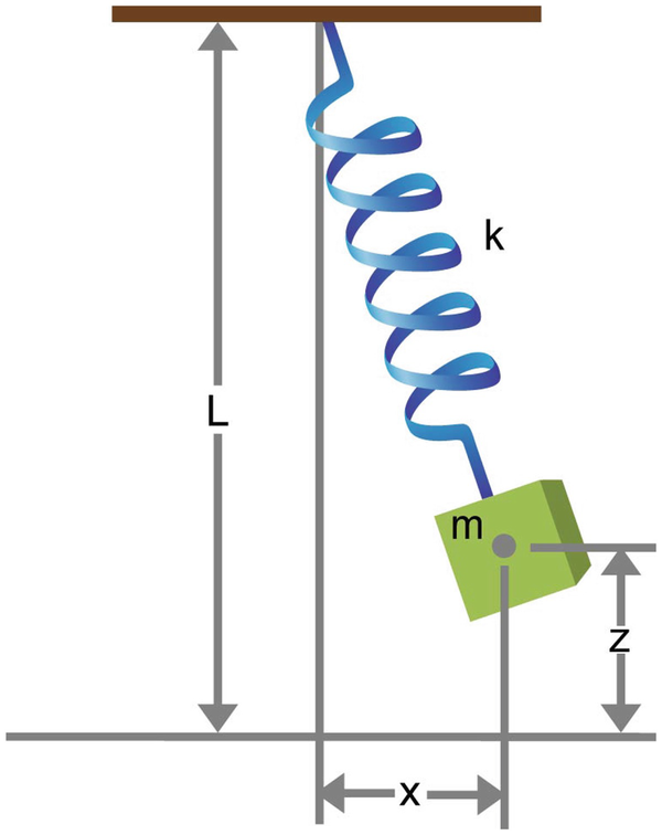

  

  An object with mass m is attached to a spring, which, in turn, is attached to the ceiling

  Assume that all objects are sufficiently far from each other. In other words, you do not have to worry about impacts.

  Assume that there is a gravitational force g pulling the mass down, and that the normal length for the spring is l ₀.

  • (a) Assume the usual spring law, and a coefficient k. Write the equations for x″ and z″ for the system.

  • (b) Assume that air resistance has an effect on the object with mass m as a result of its movement. Assume a coefficient r for the effect of air resistance on this mass. Write an updated version of the equations you wrote above to reflect this effect.

  • (c) Instead of the usual spring force law, use the following modified law:

    $$\displaystyle \begin{aligned}\text{force} = k(\text{length} - l_{0})^{3}.\end{aligned}$$

    Write the equations for x′ and z′ for the system above.

  • (d) Assume that air resistance has an effect on the masses m as a result of its movement. Assume coefficient r for the effect of air resistance on this mass. Instead of the usual air resistance law, use the following modified law:

    $$\displaystyle \begin{aligned}\text{force} = r(\text{speed})^{3}.\end{aligned}$$

    Write a modified version of the equations you wrote above to reflect this effect.

• 3. Consider the following simple system shown in Figure 2.12.

  Fig. 2.12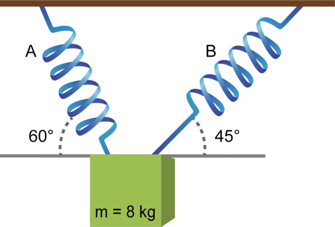

  

  An object with mass m is attached to two springs, which, in turn, is attached to the ceiling

  The diagram depicts an 8 kg mass that is hanging from two springs. The mass is subject to the effect of gravity. Assume g = 10 m/s². The mass has no other support than the springs (if they are removed, it falls). The springs are attached to the ceiling. The distance between the box and the ceiling is 1 m. We denote by k _A and k _B, the spring constants for spring A and spring B, respectively. The system is static, meaning, it is stable and there is no movement. This means that the springs are stretched, or extended so that they are each exerting a force.

  • (a) As expressions of the spring constants k _A and k _B, write the equations for the x-component and the y-component of the forces acting on the mass. Note the particular convention indicated above for axes.

  • (b) Determine the spring constants k _A and k _B.

• 4. Consider the impact of a ping pong ball with a flat floor.

  • (a) Assume that the ping pong ball is a point mass with position p = (x, y, z). Assume that the floor has infinite mass, and is horizontal. Assume further a coefficient of restitution of 0.8, meaning that the outgoing vertical speed is 0.8 of the incoming vertical speed. Write down an expression of p′ after the impact in terms of p′ before the impact.

  • (b) Now assume that the floor can have any orientation, and that the normal unit vector to the floor is N = (n _x, n _y, n _z) that is orthogonal to the surface of this floor. Note that a unit vector N has the property that ∥N∥ = 1. Write down an expression for p′ after the impact in terms of p′ before impact.

  • (c) Now assume further that the floor has mass 5 kg and the ball has mass 2 kg, and that the floor is not moving before impact. What is the speed p′ after impact?

• 5. Consider the following mechanism in Figure 2.13.

  Fig. 2.13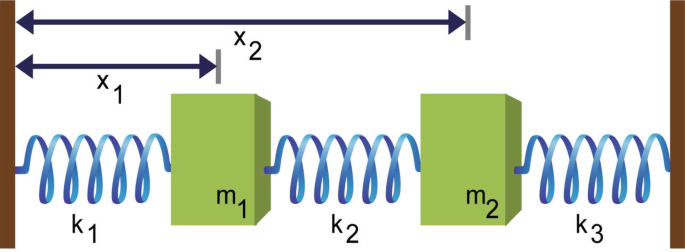

  

  A one-dimensional mechanism involving two objects and three springs

  Let the normal (unstretched) length for the springs be zero. Let u ₁ and u ₂ be input forces on each mass. Let x ₁ and x ₂ be the positions of the two masses labeled m ₁ and m ₂ as measured from the left wall. Let the right wall be at position L from the left wall. Assume the width of each mass is negligible (zero). Let k ₁, k ₂, and k ₃ be the coefficients for the three springs. Assume that all objects remain sufficiently far from each other and the two walls at all times (do not worry about impacts).

  • (a) Write down an expression for the total force acting on each of the two masses.

  • (b) Write the equations for $x_1^{\prime \prime }$ and $x_2^{\prime \prime }$, taking into account the effects of the external forces, the springs, and the inertia (mass).

  • (c) Assume u ₁ and u ₂ are zero. Write down an equation for x ₁ and x ₂ where the system can be without any motion (that is, the system is in static equilibrium).

14 Lab: Spring Bouncing and Object Creation

The purpose of this lab is to introduce us to some key modeling challenges and concepts that arise when we want to integrate both continuous and discrete dynamics. This is a good preparation for the project work and for the coming chapter.

A simple way to model a bouncing ball is that when it is away from the ground it is in free fall, and when it is touching the ground it experiences a force that we can view as the force of a spring with a high coefficient. We can call this the spring bouncing model. The following idea can be expressed as follows:

Begin this lab by sketching out the expected plots for the variables x, x', and x''. Then, run this simulation and compare it to the sketch that you had made.

An important Acumen construct used in the ping pong model is object creation. Model definitions allow us to define a type of objects. For example, we can take out parts of a model that relate to a ball from the model Main, which is a special model representing the entire world that we are simulating, to a separate model. This would lead to a model such as the following:

Now, we can easily create a world in which there are two different balls that start at different heights as soon as the world that we are simulating starts. This is done as follows:

For this lab, explore how to modify and test such a definition to: (1) how to model the presence of a damping force during the process of bouncing (this is a force that simply acts against the direction of movement), and (2) how we can introduce the effect of air resistance to a model of a moving ball.

15 Project: Mascot and Ping Pong Game

There are two parts to this chapter’s project activities: Creating a mascot for your ping pong player and familiarizing yourself with the ping pong model.

Part 1 Design a mascot for your player using Acumen. You should be able to do this after you have finished going through all the examples in the 01_Introduction directory of the Acumen distribution, and carrying out the exercises there. The mascot should consist only of a Main class and should include a _3D statement that creates the 3D form of your mascot. Once you have a good design you can consider animating the mascot or making it act in a short animation (maximum 10 s). Some examples of mascots and animations produced by past students can be found in the following online video.

Part 2 The Acumen distribution comes with a default ping pong model that can be used for the project. If you are using the book in the context of a course, your instructor may provide a custom made version of that model. The ping pong model is designed to illustrate:

• 1. Key modeling concepts that we need to know to develop almost any cyber-physical system

• 2. Basic path planning (at an intuitive level)

• 3. Basics of control

• 4. Dealing with basic mechanical features of robots

• 5. Dealing with issues such as quantization and discretization

• 6. Basic game theory

If you are not already familiar with the game of ping pong, browse through the article Table TennisTable Tennis (ping pong ) to familiarize yourself with it.

A good description of the model we will use for the project can be found in Section 6.2 of Xu Fei’s Master’s Thesis. Characteristics of this model include:

• 1. Names of included files suggest their role

• 2. Names also suggest a relation between these components (in terms of data flow). For example,

  • (a) Ball_Sensor processes Ball data going into Player

  • (b) Ball_Actuator processes signals going from Player to Bat

• 3. To learn the most from the physical modeling part of this model, it helps to do some derivation yourself starting from a 1D model of a bouncing ball to build up to a 3D. It is instructive to go over that model in detail to learn how vector and vector calculus operations are supported in Acumen.

  In the flying case, the aerodynamics part motivates the discussion of unit and norm of vectors, and some identities between them (such as what is the value of unit(p)∗norm(p), for example).

• 4. Going over the Ball_Sensor model helps in understanding sampling and how it can be modeled.

The initial model for ping pong that is used for the project can be found in the following directory:

examples/01_CPS_Course/99_Ping_Pong/Tournament1

in the Acumen distribution. Read and make sure that you understand all the files in this directory. The distribution also comes with default models for different stages of the project (called tournaments in the implementation). If you are using this textbook for a course, your instructor may also provide you with special editions of these models more closely matching the goals of the course you are following. Figure 2.14 depicts the way the ping pong model typically appears in Acumen. Numbers associated with each players are scores, and the bars on the side indicate remaining energy for the player. The white sphere is the ball itself, while the red and cyan dots are values predictions/estimates made by each player about where the ball will be at certain times. By modifying the default models provided you will both develop the design of the robot player and control how different aspects of the design are visualized in simulations.

Fig. 2.14

A typical view of ping pong model in Acumen

16 To Probe Further

• The examples presented at physicsclassroom.com

• The page by Erik Cheevers

• Background on mathematics, and physics

• You are also encouraged to watch this lecture on Rigid Body Dynamics

• Khan Academy has a great collection on basic physics

• To dig deeper, consult as needed these basic technical references on differentiation and integration, and on resistive circuit elements, analysis of resistive circuits, and RLC circuit analysis

• Sections 6.1 and 6.2 of this draft of David Morin’s book on Classical Mechanics

• For fun, you may enjoy checking out this great illustration on the scale of the universe

• Close et al.’s textbook on modeling and analysis of dynamic systems

• The Ethicist: A Heating Problem (Short article)

• Article about 17 Equations that Changed the World

• An example of a model that won a Nobel Prize: the Hodgkin-Huxkley model

• Check out Wolfram’s online Alpha tool

• Readers interested in more advanced methods for modeling mechanical systems (beyond the scope of this book) may wish to consult the article Euler-Lagrange Equation

• Much modeling and simulation aims at predicting the behavior of systems. NY Review has an interesting article on three books on prediction