Visualizing Parameter Spaces of Deep-Learning Machines

Abstract

This paper applies visualization techniques to the high-dimensional parameter spaces of a particular type of neural network, the Multi-Layer Perceptron (MLPs). MLPs are the archetypal “deep-learning” machines, digital imitations of biological brains. MLP parameter spaces are data structures holding the neuron interconnect-weights “learned” by these machines during training. These structures are abstractions of biological systems and are not generally amenable to analysis by conventional means.

The terms parameter space and (the more general) machine space will be used here interchangeably.

There are several things we would like to know about this machine as a solution to our problem, among them:

• Has our training algorithm converged “well”? (Is the trainer stuck, walking a ridge, etc.).

• Did we select the proper architecture for this classifier? (Indicated by the relative complexity of metrics in machine space).

• Did we select the proper training algorithm for this classifier? (Indicated by the regularity of the performance in machine space).

• Have we found a global optimum? (Are other optima/paths to optima visible?).

• How stable is our machine? (Are we sensitive to round-off, e.g., are we balancing on a needle?).

These questions are very difficult to answer analytically and are not very effectively addressed by sampling the feature space (e.g., blind testing). These are questions about the machine space.

Beginning with some background for those not familiar with deep-learning machines, we present a methodology for visualizing their parameter spaces, and describe how visual analysis of these spaces can inform developers.

Methods are shown for creating visual representations of performance manifolds, and how these representations assist in the characterization of certain model pathologies. In particular, performance manifolds for deep-learning machines (multi-layer perceptrons) are shown and interpreted.

1 Background

In what follows, vectors and vector-valued functions are indicated by underscoring, e.g., V, A(x); the norm of a vector is denoted | V |. The set of real numbers is denoted by R, and n-dimensional Euclidean space by R^N.

Parametric regression models are characterized by the specification of a model architecture and instantiated by the assignment of values to the model parameters. The set of all possible parameter assignments for a given model is its parameter space. For example, the parameter space for the linear functionals L(R^K) is the dual space, L * (R^K). Another example of a parameter space is R^K+1 regarded as the space of vectors of coefficients for the real polynomials of order K in the real variable x. Parameter spaces can be defined for neural networks, kernel-based classifiers, and other parametric models by unambiguously assigning each model parameter (weight, coefficient, parameter, etc.) to a dimension in some Euclidean space R^D.

Adaptive learning problems are often formulated as regressions whose values are known on some training set. For these problems, an instance from a family of functions is sought that maps each training datum to a specified target value. The development of classifiers, estimators, and a wide range of decision support problems is a parameter space search that constitutes an instance of machine learning.

Assessment artifacts like correlation tables on the input side, and confusion matrices on the output side, provide secondary measures of model operation: they can be used to assess model inputs and outputs, but not the operational processes that tie these together. Obtaining primary measures of model operation requires analysis of the parameters determining how model outputs are developed from feature inputs; it is the parameters that contain information about model stability (round-off, convergence, range problems) and model pathology (e.g., over/under parameterization, multi-co-linearity).

However, while visualization is often used to analyze, conform, and regularize input and output data, it is almost never applied to the model parameters developed, owing to their high-dimensionality and general inscrutability.

The machine learning problem can be viewed as a search of some parameter space for settings that enable a regression function to model the outputs of a decision operation. This problem can be thought of in terms of the underlying geometry of these spaces, suggesting the use of ray tracing as a method for visualizing aspects of machine learning.

A family of functions selected as candidates for a parametric regression (and so having a common domain and range) is a Model Space.

The common domain of the functions in the Model Space is called the Feature Space; it contains the sets of features to be mapped to their respective target values. The common range of the functions in the Model Space is the Goal Space; it contains the target values for the regression.

A symbolic representation of an attribute is referred to as a feature (e.g., size, quality, age, color, etc.). Features can be numbers, symbols, or complex data objects. Features are usually reduced to some simple form before modeling is performed; for the sake of definiteness, we will assume here that all features are represented by real numbers.

In the context of modeling, it is customary to identify an entity being modeled with the totality of its features (c.f., the philosophy of “Essentialism”). Once features for modeling have been selected (and coded as real numbers), a feature space can be defined by assigning each feature to a specific position in an ordered “tuple”. Each instance of an entity having the given features is then represented by a point in n-dimensional Euclidean space: its feature vector. This Euclidean space, the feature space for the domain, has dimension equal to the number of features.

When known, the target value for a feature vector is often referred to as its “ground truth”, and the set of all possible target values for a regression problem is its Goal Space. For continuous estimation problems (e.g., assigning a credit score), the Goal Space is usually a subset of R (e.g., [350, 850]). For classifiers, the Goal Space is usually an initial segment of the Natural Numbers (e.g., class identifiers 1, 2, …, M).

For many problems, building a regression model requires a set of feature vectors, each having a known target value. Machine learning methods that use such a “set having ground truth” are referred to as supervised learning methods.

The set of all vectors of parameters which instantiate a particular function in the Model Space is the Parameter Space.

Example I.

The diagram in Fig. 1 below depicts a binary (two class) classifier in a 3-dimensional Feature Space. As a two-class problem, the Goal Space is the two-point set {1, 2}.

Fig. 1.

A pictorial representation of a classification problem.

The feature vectors of the two classes have been separated by a plane. Class 1 vectors are to the left and above the plane, and Class 2 vectors are to the right and below the plane. Such a separating structure in feature space is called a “Decision Surface”.

All decision surfaces that are planes in this feature space are completely characterized by the values of the three coefficients A, B, and C; therefore, the Parameter Space for this parametric regression problem is R³.

Example II.

An estimator is desired for tomorrow’s temperature at a particular location as a function of time-of-day. A parametric regression for this modeling problem might use the following:

• Feature Space (the empirical inputs to the model): [0, 24] in hours after midnight (time-of-day)

• Goal Space (the regression outputs): real interval [−100, 130] in degrees Fahrenheit (temperature)

• Model Space (the set of regression functions): Real polynomials of degree < 6 on [0, 24]

• Parameter Space: R⁶ (ordered 6-tuples of coefficients that instantiate a polynomial regression)

Developing parametric regressions is an optimization problem, where some algebraic, iterative, or recursive technique is employed to find, for the set of points in Feature Space, a vector of parameters in the Parameter Space that instantiates a function in Model Space mapping Feature Space inputs to “correct” Goal Space outputs.

Parameters are the (usually numeric) settings necessary to make model formalisms explicit. Examples of parameters for various learning machine regressions are:

• Polynomials: Coefficients (constant multipliers for powers of the variable(s))

• Fourier Series: Fourier Coefficients (amount of energy in each frequency)

• MLP: Interconnect weights (strengths of connections between neurons)

• BBNs: conditional probability tables (conditional probabilities connecting facts to conclusions)

• Kernel-Based-classifiers (SVM, RBF): regression coefficients, base-point coordinates

• Metric (K-means, RCE, matched filters): cluster centroids and weights

To facilitate optimization, an objective function is defined on the Parameter Space. This objective function is usually a real valued function having the property that its extrema correspond to vectors of parameters whose model instances are solutions of the corresponding regression problem. In the example just given, a reasonable objective function would be the RMS error of the polynomial model; the optimization would be an algorithm (e.g., Gradient Descent) that searches Parameter space for model instances that minimize the RMS regression error. For classification problems, an oft used objective function is the percent of total instances assigned to the correct class in a training set.

2 Performance Manifolds

This section defines performance manifolds and describes them for kernel-based regression models.

A parametric regression on R^N is a real-valued function $G:R^{D} \times R^{N} \Rightarrow R$ . This notation is employed to make a distinction between the feature vectors at which the instantiated regression is evaluated $\left( {\left\{ {\left( {x_{1} , x_{2} , \ldots , x_{N} } \right)} \right\}\varepsilon R^{N} } \right)$, and the regression parameters $\left( {\left\{ {\left( {c_{1} , c_{2} , \ldots , c_{D} } \right)} \right\}\varepsilon R^{D} } \right)$ characterizing an instance of G.

Let f be a function in a Model Space, and let E be an objective function for a parametric regression problem on a training set. Define a scalar field Q by assigning to each vector in the Parameter Space the corresponding value of the objective function. The restriction of Q to a manifold in the parameter space Q is called a performance manifold for f. Each point off will generate its own performance manifold. In this paper, performance manifolds will be affine spaces of co-dimension 1 (space-separating hyperplanes).

Let T be a set of feature vectors in R^N having known ground truth for each vector (viz. supervised learning). When such a set is used for model construction, it is called a training set. Let Q be an objective function. For example, Q could be the percentage of vectors of T assigned correct regression values from this instance of G; for a continuous regression, Q could be the RMS error of G on T.

Suppose we are given a parametric regression G, a well-posed training set T of feature vectors, and an appropriate objective function Q. Then each vector of parameters p ∈ R^D has associated with it a corresponding performance score Q on that training set. $Q:R^{D} \Rightarrow R$ is a scalar field and finding an optimum instance of G is a search of R^D for extremal values of this scalar field. Such an optimum resulting from a training activity will here be called the “Best” machine.

To facilitate visualization of the field Q, which is almost always high-dimensional, we might extract and display low-dimensional affine subsets of R^D colorized by the values assumed by Q. These manifolds, which are “slices” of the parameter space colorized using the values of Q, are performance manifolds. As will be seen, visualization of these manifolds gives insight into the performance of the underlying parametric regression models.

2.1 Performance Manifolds for Kernel-Based Regressions

Performance manifolds for kernel-based regressions are relatively simple, as the following analysis for G:R × R ⇒ R illustrates.

Let x₁, x₂, …, x_N ∈ R¹be a training set, T. Let the kernel functions be F_i(x), i = 1, 2, …, D.

Define the vector-valued function F_k= (F₁(x_k), F2(x_k), …, F_D(x_k)), k = 1, 2, …, N, and let δ= (δ_0, δ_1, …, δ_0D−1 ∈ R^D.

For x ∈ R¹, let G₀ (x) = ∑_i=0,D−1 a_i F_i(x) be a regression model based on the kernel functions F_i, having coefficients a_i. Then G₀ (x) is a polynomial in x of degree D − 1. Suppose that this regression model has error 0 (i.e., it is a “Best” machine for this problem).

Let G_δ (x) = ∑_i=0,D−1 (a_i +δi) F_i(x) be the corresponding model whose i^th coefficient a_i has been perturbed by δ_i.

The modeling error introduced by perturbing the coefficients of G at x_k by can be denoted:

$$ \begin{array}{*{20}l} {E_{k} (\underline{\delta } ) = G_{0} \left( {x_{k} } \right) {-} G_{{\underline{\delta } }} \left( {x_{k} } \right) , k = 1, 2, \ldots , N} \hfill \\ {\quad = \sum_{i = 0,D - 1} a_{i} F_{i} \left( {x_{k} } \right) - \sum_{i = 0,D - 1} (a_{i} + \delta_{i} ) \, F_{i} \left( {x_{k} } \right)} \hfill \\ {\quad \quad \quad \quad = \, - \sum_{i = 0,D - 1} \delta_{i} F_{i} \left( {x_{k} } \right)} \hfill \\ {\quad \quad \quad \quad \quad \quad = - \underline{\delta } \cdot \underline{F}_{k} } \hfill \\ \end{array} $$

(1)

The RMS error of G_δ(x_k) as an approximation of G₀(x_k) over the set x₁, x₂, …, x_N ∈ R¹ is:

$$ \begin{array}{*{20}l} {\quad \quad \quad \quad E(\underline{\delta } ) = \surd \left[ {\left( {1/N} \right)\sum_{k = 1,N} (E_{k} (\underline{\delta } ))^{2} } \right]} \hfill \\ { = \, \left( {\left| {\underline{\delta } } \right|/\surd {\text{N}}} \right)\surd \left[ {\left( { 1/{\text{N}}} \right)\,\sum_{k = 1,N} \,\left\{ {\left| { F_{k} } \right|^{2} \,cos^{2} \left( {\theta_{{\underline{\delta} ,k}} } \right)} \right\}} \right]} \hfill \\ \end{array} $$

(2)

where θ_δ,k is the angle between δ and F_k in R^D. Therefore, the 2-dimensional performance manifolds of Q = E(δ) show a roughly radial symmetry, with highest performance at {a_0, a_1,…, a_D-1}, dropping off at larger distances. In Fig. 2, the error is 0 in the center where | δ | = 0, and increases with increasing | δ |. Figure 3 shows an example of how problem complexity can affect performance manifolds.

Fig. 2.

The performance manifold for a kernel-based regression has radial symmetry

Fig. 3.

Simple pictorial example showing feature space and parameter space for a binary classifier in the cartesian plane.

3 Creation of Performance Manifold Displays

In order to establish the parameter space R^D for visualizing performance manifolds for MLP’s, the model parameters can be placed in some systematic order. Here we use input layer neuron weights, hidden layer neuron weights, finally output layer weights. The topology (#layers, # neurons in each layer, and # inputs coming into each layer) must also be preserved so that the MLP can be reconstituted (Fig. 4).

Fig. 4.

Labeling they components of a multi-layer perceptron

The MLP topology must also be saved with the interconnect weights:

• # features = # inputs to each input-layer neuron = 3

• # input-layer neurons = # inputs to each hidden layer neuron = 2

• # hidden layers = 1

• # neurons in each hidden layer = # inputs to each output layer neuron = 4

• # output neurons = # classes in Goal Space = 2.

3.1 Mapping a Performance Manifold to the Computer Display

Consider the two vectors E1 and E2 in R^D:

• E₁= (1,0,1,0, …,1,0) (here D is even; if odd, the last to values would be 0,1)

• E₂= (0,1,0,1, …,0,1) (here Dis even; if odd, the last two values would be 1,0)

Given Q in R^D, we select the 2-dimensional plane that is the linear span of E₁ and E₂. The restriction of Q to this hyperplane is a performance manifold. Each point in this 2-manifold has an associated field value, given by the objective function. The “Best” machine is established as the origin of a coordinates for the display and is positioned in the center of the field of view. The line passing through the center and parallel to E1becomes the horizontal axis for the display; the line passing through the center and parallel to E2 becomes the vertical axis for the display.

Motion within the manifold parallel to the vertical axis adds or subtracts a fixed amount from all of the odd-numbered parameters of the regression (because of how E1 is defined); Motion within the manifold parallel to the horizontal axis adds or subtracts a fixed amount from all of the even-numbered parameters of the regression (because of how E2 is defined). By virtue of this coordinatization of the performance manifold, this single two-dimensional manifold captures unbiased information about the effect of every parameter, no matter how many there are, and in an intuitive way.

Motion to the left and up in this presentation causes half of the parameters to increase, and half to decrease. These changes tend to cancel out for small changes, giving most performance manifolds for well-conditioned regressions a upper-left to lower-right symmetry; along such diagonals, performance is often roughly constant… experience has shown this to be a sign of good convergence. Examples are in Sect. 5 (Fig. 5).

Fig. 5.

The slice along a “great circle” has the “best machine” at the center. This great circle disc is rendered as the “Flat” manifold.

3.2 Interpreting Performance Manifolds

Direct mathematical analysis of MLPs is difficult, but in extensive experiments on a variety of problems, the authors have made several empirical observations:

• Underdetermined MLPs (topology too simple to converge to a complete solution) tend to have

• Featureless performance manifolds and so, tiny gradients.

• Over-determined MLPs (topology more complex than necessary for convergence to a complete solution) tend to have highly-complex and isolated sub-optimal extrema.

• Local extrema appear in the manifold as isolated regions of locally high performance, “foothills” at which learning methods relying on gradient techniques (such as Back Propagation) tend to become trapped.

3.3 Streaming a Sequence of Manifolds as Movie Frames to Analyze Parameter Space Context

Even before being mapped to a 2-dimensional display, our “flat” performance manifolds are informed only by a slice of the parameter space, limiting their information content. These displays provide no information about what is happening away from the screen hyperplane. What is really needed is a means of visualizing the “depth” of the parameter space in a neighborhood of the “Best” machine. This requires multiple slices. This can be achieved by arranging a sequence of “flat” manifolds as the frames of an animation, showing how performance changes as the viewer approaches the “Best” machine from a distance in the parameter space.

The basic idea is very simple: instead of just a single N − 1 slice of parameter space, colorized sequences of N − 1 dimensional spherical surfaces converging to the training solution are visualized in a movie. Each frame is rendered as a ray traced frame. The frames are then sequenced and merged an animated gif.

One vexing technical conundrum is how to hold constant the area being visualized, since the field of view shrinks to zero as the viewer approaches the “Best” machine at the core of the manifold. Our solution is to move the screen plane closer to the center of the ball at the rate necessary to keep its apparent size constant (Fig. 6).

Fig. 6.

Reduce the field-of-view to compensate for the decreasing image size

3.4 Animating the Approach Through Parameter Space to an “Optimal” Machine

The following example shows the view as a series of smaller and smaller nested spherical “shells” are penetrated on the approach to the “Best” machine at their center. This was produced by ray tracing the performance manifold of a three-layer MLP with nine feature inputs, five nodes in the hidden layer, and two nodes in the output layer.

The MLP was trained and the graphic was produced by processing a blind hold-back set. The performance of the machine is determined as the classification accuracy on the entire blind set; this value (in the range 0% to 100%) is linearly mapped to one of four gray values for the rendering. In the gray scale version of the performance manifold, the color gradients are in 25% increments from white to black, with light gray being the absolute best machine.

For this example, the Performance Manifold generated 250 frames of animation in 2 h on a core I7 Intel based computer with 6 gigabytes of DDR 3600 MHz memory with a Windows 7 64-bit Operating System.

Figure 7 below are frames from movies depicting a hyperspace approach to the optimized machine by ray-cast animation of the hyper-spherical performance manifolds with continuously decreasing radius.

Fig. 7.

Far-away from the “Best” machine at the center of the ball, regions of both low performance (dark) and high performance (light) are present. The low-performance regions shrink and are left behind as the viewer approaches the “Best” machine at the center of the ball.

4 Some Empirical Experiments for Different Classifiers and Data Sets

For one set of experiments, four data sets were used, each having a different level of classification difficulty (as determined by an ambiguity score).

The data sets were:

• The UC Irvine Breast Cancer Data Set (Very Easy)

• Synthesized clusters having moderate overlap (Moderately easy)

• Prediction of the number of valence electron of an element based upon several of its physical properties (melting point, etc.) (Difficult)

• The parity-9 problem (Very Difficult)

Four classifiers, each using a different paradigm, were applied to each data set. The classifiers were:

• Linear Discriminant (weak)

• Nearest neighbor (weak)

• Maximum Likelihood (strong)

• Multi-Layer Perceptron (very strong)

As expected, the performance manifolds for weaker classifiers present a less variegated visual scene. More powerful classifiers present a textural complexity (indicating complex interactions between model parameters), local extrema, etc. It is not possible to include samples of all these investigations here.

4.1 Additional Experiments

In Fig. 8, the same MLP topology was used to train a “Best” machine for four problems of varying complexity. The figure depicts performance manifolds at the same fixed distance from the “Best” instance of this MLP for each problem. White represents the highest performance, with successively darker colors indicating lower performance. As suggested earlier in Fig. 3, harder problems tend to have smaller regions of high performance, other factors being equal.

Fig. 8.

Harder problems have smaller regions of high performance

5 Performance Manifolds and Modeling Problems

As with other regression formalisms, numerical adequacy, model stability, and model Error for an MLP show up in the regression parameters, and so, in performance manifolds. Certain visual artifacts in displays of performance manifold often indicate specific pathologies. Some of these pathologies are:

• Under-parameterization: the MLP architecture used lacks sufficient representational power to discriminate between the ground-truth classes. Either the number of layers or number of artificial neurons should be increased.

• Over-parameterization: the MLP architecture used has more parameters than needed to discriminate between the ground-truth classes. It is over-fitting and/or modeling random error in addition to data. Either the number of layers or number of artificial neurons should be decreased.

• There are multi-collinearities among the input features. That is, the features are not linearly independent, but related by some simple rule. Because MLP’s use linear combinations during computation, features related in this way are redundant, introducing additional complexity without adding information.

5.1 Visual Analysis of Performance Manifolds for Trained MLPs

Once training is complete (takes about 3 min or so), the machine generates two performance manifolds: one colorized by the %-accuracy of the machines surrounding the “BEST” one found, and the other colorized by the precision metric of the machines surrounding the “BEST” one we found. Each pixel in the display represents an entire neural network near the “BEST” one found during training.

It is the left-hand plot that colors machines by their “Geometric Accuracy”. The right-hand plot colors machines by the percentage of the data they classified correctly. The “BEST” machine is in the center of each plot.

The trained MLP is also applied to the Blind Set (data not used to train the MLP), and the same two performance manifolds are produced. If training has been successful, the performance manifolds for the Blind Set will be very similar to the corresponding plots for the Training Set.

Example A. 3 layers, 4 features, 3 layer-1 neurons, 7 hidden layer neurons, 4 output neurons.

File: AxeT_L3F4I3H7C4, four linearly independent, linearly separable clusters.

Observations: Feature data for consists of four uniform random, 25-member clumps of radius 0.25 in 3-space positioned at the basis vectors and origin. That is, Clump 1 has GT = 1, with centroid ~(0,0,0); Clump 2 has GT = 2, with centroid ~(1,0,0); Clump 3 has GT = 3, with centroid ~(0,1,0); and Clump 4 has GT = 4, with centroid ~(0,0,1). The classes can be separated using 2-dimensional planes as decision surfaces, and the clump centroids are virtually uncorrelated (Fig. 9).

Fig. 9.

Typical symmetry, connectedness, and simplicity for a well-posed classifier

Example B. 3 layers, 4 features, 3 layer-1 neurons, 7 hidden layer neurons, 4 output neurons.

Feature data for SQUARE.csv is a regular 17 × 34 grid (x, y) in the unit square. Its GT is: 1 + int(0.5 + 2 * (x + y)).

Observations: The ground truth for this is a quadratic relationship between the two input features; this relationship can be seen in the warping of the performance manifold for precision on the left. It is also evident in the fine structure of the %-accuracy manifold on the right, though this is unlikely to be visible in a printed copy. Once again, the symmetry of the display is from upper-left to lower-right (Fig. 10).

Fig. 10.

Quadratic interrelationship among features visible in the performance manifold

Example C. 3 layers, 4 features, 5 layer-1 neurons, 11 hidden layer neurons, 2 output neurons.

File: 2x2B_L3F4I5H11C2, Multicollinearity present.

Feature data uniform random (x, y, z, w) in unit 4-cube, with x + y=z + w. GT random binary {1, 2}.

Observations: This data set was created by intentionally introducing multicollinearity into the feature vectors: the sum of features 1 and 2 equals the sum of features 3 and 4. This type of information redundancy has been observed to introduce many linear artifacts into the performance manifold, as the linear relationship in feature space cascades through the neurons of the MLP, showing up as lines of constant performance, but at varying slopes. The upper-left to lower-right symmetry has been destroyed (Fig. 11).

Fig. 11.

Loss of symmetry and linear artifacts strong multicollinearity among features

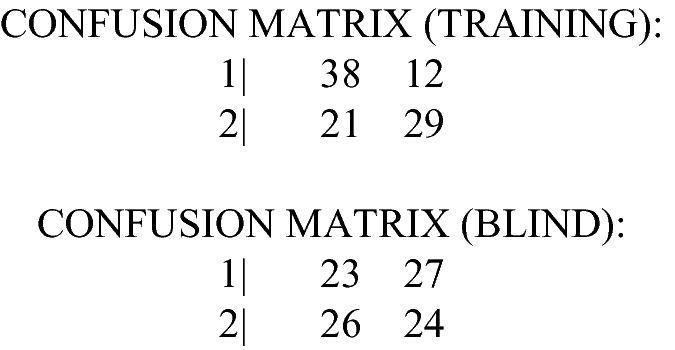
Example D1. 2 layers, 4 input features, 4 layer-1 neurons, no hidden layer, 2 output neurons.

File: rndB_L2F4I4H0C2, Under-Determined MLP Topology (too few layers and/or neurons).

Observations: The two ground truth classes were assigned randomly. This was done so that any significant patterns that might appear in the performance manifolds would result from the machine’s topology rather than patterns in the input feature vectors. Notice that the machine makes some headway in classifying the training data; but this disappears in the blind test, as it must for random ground truth.

Notice also that the strongest (brightest) visual artifacts in this display run from lower-left to upper-right, the reverse of the pattern occurring in well-conditioned architectures (Fig. 12).

Fig. 12.

Rigid, non-standard structure suggests MLP is under-determined

Performance on Blind Set:

• Accuracy: 47%

• Class1 precision: 53.1%

• Class2 precision: 47.1%

• Class1 recall: 46%

• Class2 recall: 48%

  

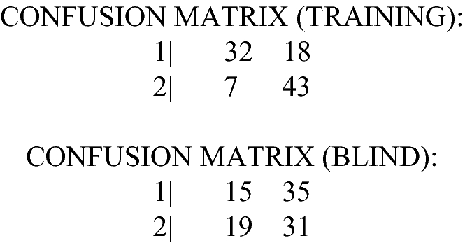
Example D2. 4 layers, 4 input features, 2 layer-1 neurons, 5 hidden layer neurons, 2 output neurons.

File: rndB_L4F4I2H5C2, Well-determined MLP Topology (right number of layers and neurons).

Observations: The performance manifold indicates that this architecture is well-conditioned for this problem. It begins to make headway on the training set, and even for the Blind data, it manages to produce elevated recall for Class2 vectors… better than expected for a random ground truth assignment.

Primary symmetry is upper-left to lower-right (Fig. 13).

Fig. 13.

Typical symmetry, connectedness, and simplicity for a well-posed classifier

Performance on Blind Set:

• Accuracy: 46%

• Class1 precision: 44.1%

• Class2 precision: 47.0%

• Class1 recall: 30%

• Class2 recall: 62%

  

Example D3. 5 layers, 4 input features, 6 layer-1 neurons, 13 hidden layer neurons, 2 output neurons.

File: rndB_L5F4I6H13C2,Over-determined MLP Topology (too many layers and or neurons).

Observations: Over-parameterization (too many layers, too many neurons) caused the performance manifold to bifurcate, with the upper branch having smooth gradient, and the lower riddled with a complex distribution of local extrema. A gradient technique would likely not be able to traverse the lower branch… and this is the branch containing the “Best” machine. As is often the case, this over-determined machine controls the training set well; but this is misleading, because this performance does not generalize to blind data. Primary symmetry is upper-left to lower-right (Fig. 14).

Fig. 14.

Bifurcated into a stable band, and a chaotic band. Suggests MLP is over-determined.

Performance on Blind Set:

• Accuracy: 50%

• Class1 precision: 50%

• Class2 precision: 50%

• Class1 recall: 48%

• Class2 recall: 52%

6 Conclusions

• All modeling involves at least three spaces: feature space, where the empirical data resides; goal space, where the ground-truth resides; and machine space, where the regression parameters reside.

• We usually think of doing modeling in the feature space. But models themselves can be modeled (meta-modeling) by applying modeling techniques to their machine spaces.

• Valuable information about machine architectures, training, and performance can be gained by meta-modeling.

We usually think of modeling in the feature space. However, models themselves can be modeled (meta-modeling) by applying modeling techniques to the parameter spaces. Valuable information about machine architectures, training, and performance can be gained by forensic meta-modeling. In particular, the use of ray cast animation in N-dimensional space makes possible direct, intuitive forensic analysis of learning machine implementations. Important phenomena can be direct observed in this way, such as:

• The presence and distribution of local extrema of the objective function used for machine learning

• Adequacy of the learning architecture.

7 Future Work

• Build a user interface that facilitates direct interact with the parameter/machine space. Functionality would include zooming in and out and spin the sphere to discover the range of solutions for the machine. Allow the user to manually “game” the coloration: adjusting the color boundaries of the model by accuracy to see how accurate a machine can get before it is not efficient.

• Use described visual methods not just for forensics, but for design as well. In an interface similar to the one described above, a user could be given the ability to select a machine by mouse click.

• Optimize the rendering process for speed to support direct user interaction.

• Additional cross-paradigm experimentation using other reasoning paradigms, such as Self Organizing Maps.

• Use for analysis of known pathologies (such as local extrema).

References

Appel, A.: Some techniques for shading machine renderings of solids. In: Proceedings of AFIPS JSCC, vol. 32, pp. 37–45 (1968)
Arbib, M.A.: Handbook of Brain Theory and Neural Networks, pp. 157–160. Bradford Books, MIT Press, Cambridge (2002)
Cortes, C., Vapnik, V.: Support-vector networks. Mach. Learn. 20(3), 273–297 (1995)
Delmater, R., Hancock, M.: Data Mining Explained, pp. 145–146. Digital Press, Newton (2001)
Hancock, M.: Near and long-term load prediction using radial basis function networks. In: Progress in Neural Processing, vol. 5, pp. 113–114. World Scientific (1995)
Haykin, S.: Neural Networks: A Comprehensive Foundation, 2nd edn. Prentice Hall, Upper Saddle River (1998)
Leondes, C.T.: Knowledge-Based Systems: Techniques and Applications, vol. 2, 1st edn, p. 436. Academic Press, San Diego (2000)
Pearl, J., Russell, S.: Bayesian Networks, Handbook of Brain Theory and Neural Networks. MIT Press, Cambridge (2001)
Winkler, K.P. (ed.): Locke, John, An Essay Concerning Human Understanding, pp. 33–36. Hackett Publishing Company, Indianapolis (1996)
Acknowledgements
The authors would like to thank the Sirius Project for facilitating this research. The Principal Author would like to thank Aneta Compton for her contribution to making this work possible.
Author information
Authors and Affiliations
Corresponding authors
Editor information
Editors and Affiliations
Rights and permissions
Copyright information
© 2019 Springer Nature Switzerland AG
About this paper
Cite this paper
Hancock, M. et al. (2019). Visualizing Parameter Spaces of Deep-Learning Machines. In: Schmorrow, D., Fidopiastis, C. (eds) Augmented Cognition. HCII 2019. Lecture Notes in Computer Science(), vol 11580. Springer, Cham. https://doi.org/10.1007/978-3-030-22419-6_15
Download citation
DOI: https://doi.org/10.1007/978-3-030-22419-6_15
Published:
Publisher Name: Springer, Cham
Print ISBN: 978-3-030-22418-9
Online ISBN: 978-3-030-22419-6
eBook Packages: Computer ScienceComputer Science (R0)