Identity-Based Functional Encryption for Quadratic Functions from Lattices

Abstract

We present a functional encryption scheme for quadratic functions from lattices under identity-based access control. This represents a practical relevant class of functions beyond multivariate quadratic polynomials and may adapt to many scenarios. Recently, Baltico et al. [10] in Crypto 2017 presented two constructions from pairings which enable efficient decryption only when $\mathbf {x}^\top \mathbf {F}\mathbf {y}$ is contained in a sufficiently small interval to finally compute a discrete logarithm, and one construction is proved selectively secure under standard assumptions and the other adaptively secure in the generic group model (GGM). Our construction is no pairings and no small interval restriction. We formalize the definition of identity-based functional encryption and its indistinguishability security and achieve adaptive security against unbounded collusions under standard assumptions in the random oracle model.

Supported by National Natural Science Foundation of China grants No. 61772514, No. 61472414, No. 61602061, and National Key R&D Program of China (2017YFB1400700).

1 Introduction

Functional Encryption (FE) is an ambitious generalization of public-key encryption which overcomes the all-or-nothing, user-based access to encrypted data and enables fine grained, role-based access to the data. Namely, functional encryption comes equipped with a key generation algorithm that utilizes a master secret key to generate decryption keys $sk_F$ corresponding to functions F, the key holders only learn F(x) from a ciphertext Enc(x) and no more information about x is revealed. This is well suited for cloud computing platforms and remote untrustworthy severs to store sensitive private data and allow users to request the result of the function F computing on the underlying data.

The definition of functional encryption was first formalized by [17, 39] which gave indistinguishability (IND-based) and simulation (SIM-based) security model, and identity-based encryption (IBE) [2, 14, 15, 20, 21, 28, 44], attribute-based encryption (ABE) [11, 16, 31, 33, 42], predicate encryption (PE) [3, 32, 35, 36, 38] and other concrete functionalities [18, 45] in a general framework could all be regarded as specific function classes of functional encryption.

Though Garg et al. [9, 24, 26, 46] constructed functional encryption for general function, their work used brilliant but ill-understood indistinguishability obfuscation(iO) or multi-linear maps machinery that existing constructions [23, 27] were found to be insecure [22, 34], so there is no provably secure instantiation by now. Some work [4, 5, 29, 30] considered general function under bounded collusions from simple primitives or well-understood assumptions. Conversely, there is also some fascinating work that constructs iO from FE schemes [8, 12, 13, 25].

Recently Abdalla et al. [1] built FE for linear functions surprisingly and efficiently from standard assumptions like the Decision Diffie-Hellman (DDH) and Learning-with-Errors (LWE) assumptions. Later, Agrawal et al. [4] promoted their schemes from selective security to adaptive security and gave an additional construction from Decision Composite Residuosity (DCR) assumption. Beyond linear functions, Baltico et al. [10] constructed two FE schemes for quadratic functions from pairings which enable efficient decryption only when $\mathbf {x}^\top \mathbf {F}\mathbf {y}$ is contained in a sufficiently small interval to finally compute a discrete logarithm, and one construction is proved selectively secure under standard assumptions and the other adaptively secure in the generic group model (GGM). This motivates the following question:

Can we build adaptively secure FE scheme for quadratic functions without pairings and the small interval restriction?

1.1 Our Results

We answer the above question affirmatively. We propose the first adaptively secure FE scheme for quadratic functions from lattices against unbounded collusions, but under identity-based access control. On the one hand, identity-based functional encryption can be regarded as functional encryption under identity-based control. On the other hand, we can think it as an extension of identity-based encryption what only allow certain identity owner to decrypt partial information or function values. We notice that Sans and Pointcheval [43] consider the identity-based access control as an additional property to expand the possible applications of their unbounded length inner product FE schemes. Here we formalize the identity-based functional encryption definition and indistinguishability security (IND-IBFE-CPA) based on [17, 39]. Namely, we additionally add identity id to the input to KeyGen and Encrypt algorithms, and we need the identity-based access control property to prove adaptive security of our scheme under random oracle model. So constructing adaptively secure FE scheme for quadratic functions under standard model is still an open problem.

In recent years, lattice-based cryptography has been shown to be extremely versatile, leading to a large number of attractive theoretical applications. Lattice problems provide some significant advantages not found in other types of cryptography, based on worst-case assumption, resistant to cryptanalysis by quantum algorithms and lattice cryptography operations are very simple (almost matrix operations), especially to our scheme, without the small interval restriction to finally compute a discrete logarithm. We employ preimage sampling techniques with trapdoor [2, 20, 28] to generate secret keys unlike linear functions schemes from LWE assumption [4] which do not use preimage sampling algorithms with trapdoor.

Overview of Techniques.

We utilize $\mathbf {x}^\top \mathbf {F}\mathbf {y}$ form to represent general quadratic functions the same as [10]. Without loss of generality, messages are expressed as pairs of vectors $(\mathbf {x}, \mathbf {y}) \in \mathbb {Z}^l \times \mathbb {Z}^l$ of the same length l, and it is easy to see that the case in which one is longer than the other can be captured by padding the shorter one with zero entries, and secret keys are associated with ($l \times l$) matrices $\mathbf {F}$, and decryption allows to compute $\mathbf {x}^\top \mathbf {F}\mathbf {y}=\sum _{i, j} f_{i, j} x_{i} y_{j}$.

We use dual Regev’s cryptosystem for multi-bit messages [4, 28], which enjoys ciphertexts have size O(l). Namely, we set $Ct_{(\mathbf {x},\mathbf {y})}=(\mathbf {c}_{01}, \mathbf {c}_{02}, \mathbf {c}_{11}, \mathbf {c}_{12})$:

where $\mathbf {s}_1, \mathbf {s}_2$ are chosen at random, $\mathbf {U}_{1}, \mathbf {U}_{2}$ are $\mathbb {Z}^{n \times l}_{q}$ matrices, and $\mathbf {A}, \mathbf {B}\in \mathbb {Z}^{n \times m}_{q}$ are contained in the public key and $\mathbf {r}_{1}, \mathbf {r}_{2}, \mathbf {r}_{1}^{'}, \mathbf {r}_{2}^{'}$ are noises. We have a relation that $\mathbf {A}\mathbf {E}_{1}=\mathbf {U}_{1}, \mathbf {B}\mathbf {E}_{2}=\mathbf {U}_{2}$ where $\mathbf {E}_{1}, \mathbf {E}_{2}\in \mathbb {Z}^{m \times l}$ are sampled uniformly from discrete Gaussian probability distributions. We observe that

$$\begin{aligned} \mathbf {x}^\top \mathbf {F}\mathbf {y} \approx \mathbf {c}_{02}^{\top }\mathbf {F}\mathbf {c}_{12} -\mathbf {c}_{01}^{\top }\mathbf {E}_{1}\mathbf {F} \mathbf {c}_{12}-\mathbf {c}_{02}^{\top }\mathbf {F} \mathbf {E}_{2}^{\top }\mathbf {c}_{11}+\mathbf {c}_{01}^{\top } \mathbf {E}_{1}\mathbf {F}\mathbf {E}_{2}^{\top }\mathbf {c}_{11}. \end{aligned}$$

Thus we set $sk_{\mathbf {F}}=(\mathbf {F}, \mathbf {E}_{1}\mathbf {F}, \mathbf {F}\mathbf {E}_{2}^{{\top }}, \mathbf {E}_{1}\mathbf {F}\mathbf {E}_{2}^{{\top }})$. Then, there is a problem that if one user asks for an $\mathbf {F}$ which is invertible (especially unitary matrix), he will get a pair of $\mathbf {E}_{1}, \mathbf {E}_{2}$ from $sk_{\mathbf {F}}$ and he can compute arbitrary $sk_{\mathbf {F}'}=(\mathbf {F}', \mathbf {E}_{1}\mathbf {F}', \mathbf {F}'\mathbf {E}_{2}^{{\top }}, \mathbf {E}_{1}\mathbf {F}'\mathbf {E}_{2}^{{\top }})$ corresponding to $\mathbf {F}'$ and decrypt arbitrary $\mathbf {x}^\top \mathbf {F}'\mathbf {y}$ owing to the relation that $\mathbf {A}\mathbf {E}_{1}=\mathbf {U}_{1}, \mathbf {B}\mathbf {E}_{2}=\mathbf {U}_{2}$ always holds.

To circumvent this problem, we employ extension preimage sampling techniques with trapdoor [2, 20]. We additionally use a public matrix $\mathbf {R} \in \mathbb {Z}^{n \times l}_q$ to randomize $\mathbf {F}$ and make the multiplication into the extension preimage sampling algorithms. So in the KeyGen algorithm, the relation becomes $(\mathbf {A}|\mathbf {R}\mathbf {F})\mathbf {E}_{1}=\mathbf {U}_{1}$ and $(\mathbf {B}|\mathbf {R}\mathbf {F})\mathbf {E}_{2}=\mathbf {U}_{2}$ where $\mathbf {E}_{1}, \mathbf {E}_{2}\in \mathbb {Z}^{(m+l) \times l}$ can be sampled uniformly by extension sampling algorithms with trapdoors $T_{\mathbf {A}}, T_{\mathbf {B}}$.

In order to prove the security, we need to regard $\mathbf {U}_{1}, \mathbf {U}_{2}$ as random oracle $\mathbf {U}_{1}(id), \mathbf {U}_{2}(id)$: $\{0, 1\}^{*} \rightarrow \mathbb {Z}^{n \times l}_{q}$ to answer secret keys queries for arbitrary identity id except the challenge $id^*$ and arbitrary $\mathbf {F}$. For different $\mathbf {F}$, there are distinct $\mathbf {E}_{1}, \mathbf {E}_{2}$ which have enough entropy to resist collusion attacks.

1.2 Related Work

Agrawal and Rosen [5] considered bounded collusions schemes from LWE assumption, and they also achieved bounded collusions functional encryption for quadratic functions.

Sans and Pointcheval [43] consider the identity-based access control as an additional property to expand the possible applications of their unbounded length inner product FE schemes. They do not formalize the definition of identity-based functional encryption and its security model, and they only achieve selective security from pairings under random oracle model for their unbounded length inner product FE schemes.

1.3 Organization

In Sect. 2, we introduce some necessary notations and some lemmas, algorithms and assumptions from lattice-based cryptography. We formalize the definitions of identity-based functional encryption (IBFE) and its security model in Sect. 3. Section 4 presents our IBFE scheme for quadratic functions. In Sect. 5, we analyze the security of our scheme. We conclude and propose some open problems in Sect. 6.

2 Preliminary

Notations. We denote vectors by lower-case bold letters (e.g. $\mathbf {x}$) and are always in column form (respectively, $\mathbf {x}^{\top }$ is a row vector). Matrices are denoted by upper-case bold letters (e.g. $\mathbf {A}$) and treat them with their ordered column vector sets $[\mathbf {a}_1,\mathbf {a}_2,...]$. We let $\mathbf {M_1} | \mathbf {M_2}$ denote the (ordered) concetenation of the column vector sets of $\mathbf {M_1}$ and $\mathbf {M_2}$, $\mathbf {M_1} \Vert \mathbf {M_1}$ denote the (ordered) concetenation of the row vector sets of $\mathbf {M_1}$ and $\mathbf {M_2}$, and vectors are similar. For a vector $\mathbf {x}$, we let $\Vert \mathbf {x} \Vert$ denote its $l_2$ norm and $\Vert \mathbf {x} \Vert _{\infty }$ denote its infinity norm. Similarly, for matrices $\Vert \cdot \Vert$ and $\Vert \cdot \Vert _{\infty }$ denote their $l_2$ and infinity norms respectively.

2.1 Functional Encryption

We recall the syntax of functional encryption, as defined by [17], and their indistinguishability based security definition.

Definition 1

(Functionality). A functionality F defined over ($\mathcal {K}$, $\mathcal {M}$) is a function F : $\mathcal {K} \times \mathcal {M} \rightarrow \varSigma \cup \{\bot \}$ where $\mathcal {K}$ is a key space, $\mathcal {M}$ is a message space and $\varSigma$ is an output space which does not contain the special symbol $\bot$.

Definition 2

(Functional Encryption). A functional encryption scheme FE for a functionality F is a tuple of four algorithms FE = (Setup, KeyGen, Encrypt, Decrypt) that work as follows:

• Setup($1^{\lambda }$) takes as input a security parameter $1^{\lambda }$ and outputs a master key pair (mpk, msk).

• KeyGen(msk, K) takes as input the master secret key and a key (i.e. a function) K $\in \mathcal {K}$, and outputs a secret key $sk_K$.

• Encrypt(mpk, M) takes as input the master public key mpk and a message M $\in \mathcal {M}$, and outputs a ciphertext C.

• Decrypt($mpk, sk_K, C$) takes as input a secret key $sk_K$ and a ciphertext C, and returns an output $v \in \varSigma \cup \{\bot \}$.

For correctness, it is required that for all (mpk, msk) $\leftarrow$ Setup($1^{\lambda }$), all keys K $\in \mathcal {K}$ and all messages M $\in \mathcal {M}$, if $sk_K \leftarrow$ KeyGen(msk, K) and C $\leftarrow$ Encrypt(mpk, M), then it holds with overwhelming probability that Decrypt($sk_K$, C) = F(K, M) whenever F(K, M) $\ne \bot$.

Indistinguishability-Based Security. For a functional encryption scheme FE for a functionality F over ($\mathcal {K}$, $\mathcal {M}$), security against chosen-plaintext attacks (IND-FE-CPA, for short) if no PPT adversary has non-negligible advantage in the following game:

• 1. The challenger runs (mpk, msk) $\leftarrow$ Setup($1^{\lambda }$) and gives mpk to $\mathcal {A}$.

• 2. The adversary $\mathcal {A}$ adaptively makes secret key queries. At each query, $\mathcal {A}$ chooses a key K $\in \mathcal {K}$ and obtains $sk_K \leftarrow$ KeyGen(msk, K).

• 3. Adversary $\mathcal {A}$ chooses a pair of distinct messages $M_0$, $M_1 \in \mathcal {M}$ such that F(K, $M_0$)=F(K, $M_1$) holds for all Keys K queried in the previous phase. The chanllenger computes C* $\leftarrow$ Encrypt(mpk, $M_{\beta }$) and return C* to $\mathcal {A}$.

• 4. Adversary $\mathcal {A}$ makes further secret key queries for arbitrary keys K $\in \mathcal {K}$, but under the requirement that F(K, $M_0$)=F(K, $M_1$).

• 5. Adversary $\mathcal {A}$ eventually outputs a bit $\beta ' \in \{0, 1\}$ and wins if $\beta '=\beta$.

The adversary’s advantage is defined to be $Adv_{\mathcal {A}}(\lambda )$:= $|Pr[\beta '=\beta ]-1/2|$.

2.2 Lattices

An m-dimensional lattice $\mathcal {L}$ is a discrete additive subgroup of $\mathbb {R}^m$. Given positive integers n, m, q and a matrix $\mathbf {A} \in \mathbb {Z}^{n \times m}_{q}$, we let $\varLambda _q^{\perp }(\mathbf {A})$ denote the lattice $\{ \mathbf {x} \in \mathbb {Z}^m : \mathbf {A} \cdot \mathbf {x} = \mathbf {0}$ mod $q\}$ and $\varLambda _q(\mathbf {A})$ denote the lattice $\{ \mathbf {y} \in \mathbb {Z}^m : \mathbf {y}=\mathbf {A}^{\top } \cdot \mathbf {s}$ mod q for some $\mathbf {s}\in \mathbb {Z}^n \}$. For $\mathbf {u} \in \mathbb {Z}_q^n$, we let $\varLambda _q^{\mathbf {u}}(\mathbf {A})$ denote the coset $\{ \mathbf {x} \in \mathbb {Z}^m : \mathbf {A} \cdot \mathbf {x} = \mathbf {u}$ mod $q\}$. Note that if $\mathbf {t} \in \varLambda _q^{\mathbf {u}}(\mathbf {A})$ then $\varLambda _q^{\mathbf {u}}(\mathbf {A}) = \varLambda _q^{\perp }(\mathbf {A})+\mathbf {t}$ and hence $\varLambda _q^{\mathbf {u}}(\mathbf {A})$ is a shift of $\varLambda _q^{\perp }(\mathbf {A})$.

Discrete Gaussians. Let $\sigma$ be any positive real number, $\mathbf {c}\in \mathbb {R}^m$. The Gaussian distribution $\mathcal {D}_{\sigma , \mathbf {c}}$ centered at $\mathbf {c}$ with parameter $\sigma$ is defined by the probability distribution function $\rho _{\sigma , \mathbf {c}}(\mathbf {x})=exp(-\pi \Vert \mathbf {x}-\mathbf {c}\Vert ^2/\sigma ^2)$. For any set $\mathcal {L} \subset \mathbb {R}^m$, define $\rho _{\sigma , \mathbf {c}}(\mathcal {L})=\sum _{\mathbf {x}\in \mathcal {L}} \rho _{\sigma , \mathbf {c}}(\mathbf {x})$. The discrete Gaussian distribution $\mathcal {D}_{\mathcal {L}, \sigma , \mathbf {c}}$ over $\mathcal {L}$ centered at $\mathbf {c}$ with parameter $\sigma$ is defined by the probability distribution function $\rho _{\mathcal {L}, \sigma , \mathbf {c}}(\mathbf {x}) = \rho _{\sigma , \mathbf {c}}(\mathbf {x})/\rho _{\sigma , \mathbf {c}}(\mathcal {L})$ for all $\mathbf {x}\in \mathcal {L}$.

The following lemma states that the total Gaussian measure on any translate of the lattice is essentially the same.

Lemma 1

[28, 37]. For any m-dimensional lattice $\varLambda$, $\sigma \ge \omega (\sqrt{\log m})$, $\mathbf {c}\in \mathbb {R}^m$, $\epsilon \in (0, 1)$, we have

$$\begin{aligned} \rho _{\sigma , \mathbf {c}}(\varLambda ) \in \left[ \frac{1-\epsilon }{1+\epsilon }, 1\right] \cdot \rho _{\sigma }(\varLambda ) \end{aligned}$$

A sample from a discrete Gaussian with parameter $\sigma$ is at most $\sqrt{m}\sigma$ away from its center $\mathbf {c}$ with overwhelming probability.

Lemma 2

[28, 37]. For any m-dimensional lattice $\varLambda$, $m > n$, center $\mathbf {c}$, $\sigma \ge \omega (\sqrt{\log m})$, we have

$$\begin{aligned} Pr[\Vert \mathbf {x}-\mathbf {c}\Vert > \sqrt{m}\sigma |\mathbf {x}\leftarrow \mathcal {D}_{\varLambda , \sigma , \mathbf {c}}] \le negl(n). \end{aligned}$$

There is an upper bound on the probability of a discrete Gaussian, equivalently, it is a lower bound on the min-entropy of the distribution.

Lemma 3

[28]. For any m-dimensional lattice $\varLambda$, $\sigma \ge \omega (\sqrt{\log m})$, center $\mathbf {c}$, positive $\epsilon > 0$, and $\mathbf {x}\in \varLambda$, we have

$$\begin{aligned} \mathcal {D}_{\varLambda , \sigma , \mathbf {c}} \le \frac{1+\epsilon }{1-\epsilon } \cdot 2^{-m}. \end{aligned}$$

In particular, for $\epsilon < \frac{1}{3}$, the min-entropy of $\mathcal {D}_{\varLambda , \sigma , \mathbf {c}}$ is at least m-1.

Ajtai et al. [6, 7] showed how to sample an essentially uniform $\mathbf {A}$, along with a relatively short basis $T_{\mathbf {A}}$.

Lemma 4

Let n, q, m be positive intergers with $q > 2$ and $m \ge 5n\log q$. There is a probabilistic polynomial-time(PPT) algorithm TrapGen that outputs a pair ($\mathbf {A} \in \mathbb {Z}_q^{n \times m}$, $T_{\mathbf {A}}$ $\in \mathbb {Z}^{m \times m}$) where the distribution of $\mathbf {A}$ is statistically close to uniform over $\mathbb {Z}_q^{n \times m}$ and $\Vert T_{\mathbf {A}}\Vert \le m\cdot \omega (\sqrt{\log m})$.

Gentry et al. [28] showed that if ISIS$_{q, m, 2\sigma \sqrt{m}}$ is hard, $f_{\mathbf {A}}: \mathbb {Z}_q^{m} \rightarrow \mathbb {Z}_q^{n}$ with $f_{\mathbf {A}}(\mathbf {e})= \mathbf {A}\mathbf {e}$ mod q is one-way function, even collision resistant function where $\Vert \mathbf {e}\Vert \le \sqrt{m}\sigma$. Note that for $m> 2n\log q, \sigma > \omega (\sqrt{\log m}), f_{\mathbf {A}}$ is surjective for almost all $\mathbf {A}$, and the distribution of $\mathbf {u}= \mathbf {A}\mathbf {e}$ mod q is statistically close to uniform over $\mathbb {Z}_q^{n}$. Furthermore, fix $\mathbf {u}\in \mathbb {Z}_q^{n}$, a short basis for $\varLambda ^{\perp }(\mathbf {A})$ can be used to efficiently sample short vectors from $f_{\mathbf {A}}^{-1}(\mathbf {u})$ without revealing any information about the short basis $T_{\mathbf {A}}$.

Lemma 5

Let n, q, m be positive integers with $q\ge 2$ and $m\ge 2n\log q$. There is a PPT algorithm SamplePre that on input of $\mathbf {A} \in \mathbb {Z}_q^{n \times m}$, a basis $T_{\mathbf {A}}$ for $\varLambda _q^{\perp }(\mathbf {A})$, a vector $\mathbf {u} \in \mathbb {Z}_q^n$ and an integer $\sigma \ge \Vert \widetilde{T_\mathbf {A}}\Vert \cdot \omega (\sqrt{\log m})$, the distribution of the output of $\mathbf {e}\leftarrow \mathbf{SamplePre }(\mathbf {A}, T_{\mathbf {A}}, \mathbf {u}, \sigma )$ is with negligible statistical distance of $\mathcal {D}_{\varLambda _q^{\mathbf {u}}(\mathbf {A}), \sigma }$.

2.3 Algorithm SampleR

The preimage sampling algorithm can be easily generalized to generate preimages of matrices instead of vectors by independently running SamplePre algorithm on each column of the matrix, so we overload the notation by directly giving matrices $\mathbf {U}\in \mathbb {Z}^{n \times l}_{q}$ as inputs to the SamplePre algorithm. The following algorithm is reminiscient of the extension preimage sampling algorithm of [2, 20].

Theorem 1

Let n, q, m, l be positive integers with $q\ge 2$ and $m \ge 2n\log q$. There is a PPT algorithm SampleR that on input of $\mathbf {A} \in \mathbb {Z}_q^{n \times m}$, a basis $T_{\mathbf {A}}$ for $\varLambda _q^{\perp }(\mathbf {A})$, matrices $\mathbf {M}, \mathbf {U}\in \mathbb {Z}^{n \times l}_{q}$, and an integer $\sigma \ge \Vert \widetilde{T_\mathbf {A}}\Vert \cdot \omega (\sqrt{\log (m+l)})$ outputs $\mathbf {E}_{1} \leftarrow \mathbf{SampleR }(\mathbf {A}, \mathbf {M}, T_{\mathbf {A}}, \mathbf {U}, \sigma )$ which is with negligible statistical distance of the distribution $\mathcal {D}_{\varLambda _q^{\mathbf {U}}(\overline{\mathbf {A}}), \sigma }$ where $\overline{\mathbf {A}}=(\mathbf {A}|\mathbf {M})$.

Proof

As the process of the algorithm, we have

$$\begin{aligned} Pr[\mathbf {E}_{1}]&=Pr[\mathbf {E}_{10}]\cdot Pr[\mathbf {E}_{11}:\mathbf {E}_{10}]\\&=\rho _{\sigma }(\mathbf {E}_{10})\cdot \frac{\rho _{\sigma }(\mathbf {E}_{11})}{\rho _{\mathcal {D}^{l\times l}, \sigma } \cdot \rho _{\sigma }(\{\mathbf {E}_{11}:\mathbf {A}\mathbf {E}_{11}=\mathbf {U}-\mathbf {M}\mathbf {E}_{10}\})}. \end{aligned}$$

For a $\mathbf {t}$ satisfying $\mathbf {A}\mathbf {t}=\mathbf {U}-\mathbf {M}\mathbf {E}_{10}$, we have

$$\begin{aligned} \{\mathbf {E}_{11}:\mathbf {A}\mathbf {E}_{11}&=\mathbf {U}-\mathbf {M}\mathbf {E}_{10}\}=\mathbf {t}+\varLambda _q^{\perp }(\mathbf {A}) \end{aligned}$$

Then we have

$$\begin{aligned} \rho _{\sigma }(\mathbf {t}+\varLambda _q^{\perp }(\mathbf {A})) \in \left[ \frac{1-\epsilon }{1+\epsilon }, 1\right] \cdot \rho _{\sigma }(\varLambda _q^{\perp }(\mathbf {A})) \end{aligned}$$

for some negligible function $\epsilon$. Besides, we have

$$\begin{aligned} \rho _{\sigma }(\varLambda _q^{\mathbf {U}}(\overline{\mathbf {A}})) = \sum \rho _{\sigma }(\mathbf {E}_{1})&=\sum _{\mathbf {A}\mathbf {E}_{11} =\mathbf {U}-\mathbf {M}\mathbf {E}_{10}} \rho _{\sigma }(\mathbf {E}_{11}) \rho _{\sigma }(\mathbf {E}_{10})\\&=\sum _{\mathbf {E}_{10}\leftarrow \mathcal {D}^{l\times l}} \rho _{\sigma }(\mathbf {E}_{10}) \sum _{\mathbf {E}_{11}\leftarrow \mathcal {D}^{m\times l}, {\mathbf {A}\mathbf {E}_{11}=\mathbf {U} -\mathbf {M}\mathbf {E}_{10}}} \rho _{\sigma }(\mathbf {E}_{11})\\&=\left( \sum _{\mathbf {E}_{10}\leftarrow \mathcal {D}^{l\times l}} \rho _{\sigma }(\mathbf {E}_{10})\right) \rho _{\sigma }(\mathbf {t} +\varLambda _q^{\perp }(\mathbf {A}))\\&\in \left( \sum _{\mathbf {E}_{10}\leftarrow \mathcal {D}^{l\times l}} \rho _{\sigma }(\mathbf {E}_{10})\right) \cdot \left[ \frac{1-\epsilon '}{1+\epsilon '}, 1\right] \cdot \rho _{\sigma }(\varLambda _q^{\perp }(\mathbf {A}))\\&\in \left[ \frac{1-\epsilon '}{1+\epsilon '}, 1\right] \cdot \rho _{\mathcal {D}^{l\times l}, \sigma }\cdot \rho _{\sigma }(\varLambda _q^{\perp }(\mathbf {A})) \end{aligned}$$

for some negligible function $\epsilon '$. Thus,

$$\begin{aligned}&\rho _{\sigma }(\varLambda _q^{\mathbf {U}}(\overline{\mathbf {A}})) \in \left[ \frac{1-\epsilon '}{1+\epsilon '}, 1\right] \cdot \rho _{\mathcal {D}^{l\times l}, \sigma }\cdot \rho _{\sigma }(\varLambda _q^{\perp }(\mathbf {A}))\\&Pr[\mathbf {E}_{1}] \in \rho _{\sigma }(\mathbf {E}_{10}) \cdot \frac{\rho _{\sigma }(\mathbf {E}_{11})}{\rho _{\mathcal {D}^{l\times l}, \sigma } \cdot \left[ \frac{1-\epsilon }{1+\epsilon }, 1\right] \cdot \rho _{\sigma } (\varLambda _q^{\perp }(\mathbf {A}))}\\&\quad \quad \quad \in \left[ \frac{1-\epsilon '}{1+\epsilon '}, \frac{1+\epsilon }{1-\epsilon }\right] \cdot \frac{\rho _{\sigma }(\mathbf {E}_{10})\cdot \rho _{\sigma }(\mathbf {E}_{11})}{\rho _{\sigma } (\varLambda _q^{\mathbf {U}}(\overline{\mathbf {A}}))} \end{aligned}$$

The distribution of $\mathbf {E}_{1}$ is with negligible statistical distance of the distribution $\mathcal {D}_{\varLambda _q^{\mathbf {U}}(\overline{\mathbf {A}}), \sigma }$. This ends the proof. $\square$

2.4 Learning with Errors

We review the learning with errors (LWE) problem for the most part from [41].

We first introduce the error distribution $\chi _\alpha$, that is, the normal (Gaussian) distribution on $\mathbb {T}$ with mean 0 and standard deviation $\alpha /\sqrt{2\pi }$ having density function $\frac{1}{\alpha }exp(-\pi x^2/\alpha ^2)$. Its discretized normal distribution on $\mathbb {Z}_q$ denoted to be the distribution of $\lfloor q\cdot X\rceil$ mod q, where X is a random variable with distribution $\chi _\alpha$ and $\lfloor x \rceil$ is the closest integer to x $\in \mathbb {R}$.

The following lemma about the distribution $\chi _\alpha$ will be needed to show that decryption works correctly.

Lemma 6

[2]. Let $\mathbf {x}\in \mathbb {Z}^m$ and $\mathbf {r}\leftarrow \chi _\alpha ^m$, then the quantity $\Vert \mathbf {x}^{\top }\mathbf {r}\Vert$ treated as an integer in $[0, q-1]$ satisfies

$$\begin{aligned} \Vert \mathbf {x}^{\top }\mathbf {r}\Vert \le \Vert \mathbf {x}\Vert q\alpha \omega (\sqrt{\log m})+\Vert \mathbf {x}\Vert \sqrt{m}/2 \end{aligned}$$

with all but negligible probability in m.

For an integer $q \ge$ 2 and some probability distribution $\chi$ over q, $\mathbf {s}\in \mathbb {Z}_q^n$, define $A_{\mathbf {s}, \chi }$ to be the distribution on $\mathbb {Z}_q^n\times \mathbb {Z}_q$ of the variable ($\mathbf {a}$, $\mathbf {a}^{\top }\mathbf {s}+x$) induced by choosing $\mathbf {a}$ uniformly at random from $\mathbb {Z}_q^n$, $x\leftarrow \chi$.

Learning with Errors (Decision Version). For an integer $q=q(n)$ and a distribution $\chi$ on $\mathbb {Z}_q$, LWE$_{q, \chi }$ is to distinguish between the distribution $A_{\mathbf {s}, \chi }$ for some uniform secret $\mathbf {s}\leftarrow \mathbb {Z}_q^n$ and the uniform distribution on $\mathbb {Z}_q^n\times \mathbb {Z}_q$(via oracle access to the distribution).

Regev [41] demonstrated that for certain moduli q and Gaussian error distribution $\chi _{\alpha }$, LWE$_{q, \chi _\alpha }$ is as hard as solving several standard worst-case lattice problems using a quantum algorithm.

Theorem 2

Let $\alpha (n)\in (0, 1)$ and q(n) be a prime such that $\alpha \cdot q\ge 2\sqrt{n}$. If there exists an efficient(possibly quantum) algorithm that solves LWE$_{q, \chi _\alpha }$, then there exists an efficient quantum algorithm for approximating SIVP and GapSVP to with O(n/$\alpha$) factors in the worst case.

Peikert et al. [19, 40] showed that there is a classical reduction from GapSVP to the LWE problem.

3 Definitions of Identity-Based Functional Encryption

Definition 3

(Identity-Based Functional Encryption). An identity-based functional encryption (IBFE) scheme for a functionality F is a tuple of four algorithms IBFE = (Setup, KeyGen, Encrypt, Decrypt) that work as follows:

• Setup($1^{\lambda }$) takes as input a security parameter $1^{\lambda }$ and outputs a master key pair (mpk, msk).

• KeyGen(msk, id, K) takes as input the master secret key, an $id \in \mathcal {ID}$ and a key (a.k.a. a function) K $\in \mathcal {K}$, and outputs a secret key $sk_K$.

• Encrypt(mpk, id, M) takes as input the master public key mpk, an id $\in \mathcal {ID}$ and a message M $\in \mathcal {M}$, and outputs a ciphertext C.

• Decrypt($mpk, sk_K, C$) takes as input a secret key $sk_K$ and a ciphertext C, and returns an output $v \in \varSigma \cup \{\bot \}$.

For correctness, it is required that for all (mpk, msk) $\leftarrow$ Setup($1^{\lambda }$), all $id \in \mathcal {ID}$, all keys K $\in \mathcal {K}$ and all messages M $\in \mathcal {M}$, if $sk_K \leftarrow$ KeyGen(msk, id, K) and C $\leftarrow$ Encrypt(mpk, id, M), then it holds with overwhelming probability that Decrypt($sk_K$, C) = F(K, M) whenever F(K, M) $\ne \bot$.

Definition 4

(IND-IBFE-CPA Security). For an identity-based functional encryption scheme for a functionality F over ($\mathcal {K}$, $\mathcal {M}$), security against chosen-plaintext attacks (IND-IBFE-CPA, for short) if no PPT adversary has non-negligible advantage in the following game:

• 1. The challenger runs (mpk, msk) $\leftarrow$ Setup($1^{\lambda }$) and gives mpk to $\mathcal {A}$.

• 2. The adversary $\mathcal {A}$ adaptively makes secret key queries. At each query, $\mathcal {A}$ chooses an identity $id \in \mathcal {ID}$ and a key K $\in \mathcal {K}$ and obtains $sk_K \leftarrow$ KeyGen(msk, id, K).

• 3. Adversary $\mathcal {A}$ chooses an identity id* $\in \mathcal {ID}$ and a pair of distinct messages $M_0$, $M_1 \in \mathcal {M}$ such that F(K, $M_0$)=F(K, $M_1$) holds for all Keys K queried in the previous phase. The chanllenger computes C* $\leftarrow$ Encrypt(mpk, id*, $M_{\beta }$) and return C* to $\mathcal {A}$.

• 4. Adversary $\mathcal {A}$ makes further secret key queries for arbitrary identities id $\in \mathcal {ID}$ and keys K $\in \mathcal {K}$, but under the restriction that id $\ne$ id* and F(K, $M_0$)=F(K, $M_1$).

• 5. Adversary $\mathcal {A}$ eventually outputs a bit $\beta ' \in \{0, 1\}$ and wins if $\beta '=\beta$.

The adversary’s advantage is defined to be $Adv_{\mathcal {A}}(\lambda )$:= $|Pr[\beta '=\beta ]-1/2|$.

4 Construction of Identity-Based Functional Encryption for Quadratic Functions

Let $\mathbf {U}_{1}, \mathbf {U}_{2}: \{0, 1\}^{*} \rightarrow \mathbb {Z}^{n \times l}_{q}$ be hash functions, which can be simply seen as l maps to map id to uniform syndromes in $\mathbb {Z}^{n}_{q}$ at random and independently. For ease of exposition, we overload them as matrices.

• Setup($1^n$, $1^{l}$, P, V): Utilize TrapGen to generate $\mathbf {A}\in \mathbb {Z}^{n \times m}_{q}$ and trapdoor $T_{\mathbf {A}} \subset \varLambda _q^{\perp }(\mathbf {A})$, $\mathbf {B}\in \mathbb {Z}^{n \times m}_{q}$ and trapdoor $T_{\mathbf {B}} \subset \varLambda _q^{\perp }(\mathbf {B})$, where $\mathbf {A}, \mathbf {B}$ are statistically close to uniform, and $T_{\mathbf {A}}$, $T_{\mathbf {B}}$ $\in \mathbb {Z}^{m \times m}$. Choose $\mathbf {R} \in \mathbb {Z}^{n \times l}_q$ uniformly at random. Set $max(\Vert \mathbf {x}\Vert _{\infty }, \Vert \mathbf {y} \Vert _{\infty })=P$ and $\Vert \mathbf {F}\Vert _{\infty }=V$, $K=l^{2}P^{2}V$. Define mpk:=$\{\mathbf {A}, \mathbf {B}$, $\mathbf {R}$, K, P, V} and msk:={$T_\mathbf {A}$, $T_\mathbf {B}$}.

• Keygen($msk, id, \mathbf {F}$): Given $\mathbf {F}$, running SampleR($\mathbf {A}$, $\mathbf {R}\mathbf {F}$, $T_{\mathbf {A}}$, $\mathbf {U}_{1}(id)$, $\sigma$), SampleR($\mathbf {B}$, $\mathbf {R}\mathbf {F}$, $T_{\mathbf {B}}$, $\mathbf {U}_{2}(id)$, $\sigma$) to sample $\mathbf {E}_{1}$ and $\mathbf {E}_{2} \in \mathbb {Z}^{(m+l) \times l}$ such that $(\mathbf {A}|\mathbf {R}\mathbf {F})\mathbf {E}_{1}$ = $\mathbf {U}_{1}(id)$ and $(\mathbf {B}|\mathbf {R}\mathbf {F})\mathbf {E}_{2}$ = $\mathbf {U}_{2}(id)$. Compute and return the secret key $sk_{\mathbf {F}}=(\mathbf {F}, \mathbf {E}_{1}\mathbf {F}, \mathbf {F}\mathbf {E}_{2}^{{\top }}, \mathbf {E}_{1}\mathbf {F}\mathbf {E}_{2}^{{\top }})$.

• Encrypt(mpk, id, $(\mathbf {x}, \mathbf {y})$): Sample $\mathbf {s}_{1}$, $\mathbf {s}_{2} \leftarrow \mathbb {Z}^n_q$ uniformly at random, $\mathbf {r}_{1}^{'}$, $\mathbf {r}_{2}^{'} \leftarrow \chi ^{m}_{q, \alpha }$ and $\mathbf {r}_{1}^{''}$, $\mathbf {r}_{2}^{''}$, $\mathbf {r}_{1}$, $\mathbf {r}_{2} \leftarrow \chi ^{l}_{q, \alpha }$ and compute

  

  Then, return C := ($\mathbf {c}_{01}$, $\mathbf {c}_{02}$, $\mathbf {c}_{03}$, $\mathbf {c}_{11}$, $\mathbf {c}_{12}$, $\mathbf {c}_{13}$).

• Decrypt($mpk, sk_{\mathbf {F}}, C$): Compute $\displaystyle \mu ^{'} = \mathbf {c}_{02}^{\top }\mathbf {F}\mathbf {c}_{12}-(\mathbf {c}_{01}\Vert \mathbf {F}^{\top }\mathbf {c}_{03})^{\top }\mathbf {E}_{1}\mathbf {F}\mathbf {c}_{12}-\mathbf {c}_{02}^{\top }\mathbf {F}\mathbf {E}_{2}^{\top }(\mathbf {c}_{11}\Vert \mathbf {F}^{\top }\mathbf {c}_{13})+(\mathbf {c}_{01}\Vert \mathbf {F}^{\top }\mathbf {c}_{03})^{\top }\mathbf {E}_{1}\mathbf {F}\mathbf {E}_{2}^{\top }(\mathbf {c}_{11}\Vert \mathbf {F}^{\top }\mathbf {c}_{13})$ mod $q^{2}$ and output the value $\displaystyle \mu \in \{-K+1, ... , K-1\}$ that minimizes $\displaystyle \mid (\lfloor \frac{q}{K}\rfloor )^{2}\cdot \mu - \mu ^{'} \mid$.

4.1 Parameters and Correctness

For ease of exposition, we omit id here. Observe that

$$\begin{aligned}&\mathbf {c}_{02}^{\top }\mathbf {F}\mathbf {c}_{12}\\&=(\mathbf {U}_{1}^{\top }\mathbf {s}_1+\mathbf {r}_{1}+ \lfloor \frac{q}{K} \rfloor \cdot \mathbf {x})^{\top }\mathbf {F}(\mathbf {U}_{2}^{\top }\mathbf {s}_2+\mathbf {r}_{2}+ \lfloor \frac{q}{K} \rfloor \cdot \mathbf {y})\\&=(\mathbf {U}_1^{\top }\mathbf {s}_1)^{\top }\mathbf {F}\mathbf {U}_2^{\top }\mathbf {s}_2+(\mathbf {U}_1^{\top }\mathbf {s}_1)^{\top }\mathbf {F}\lfloor \frac{q}{K} \rfloor \cdot \mathbf {y}+(\lfloor \frac{q}{K} \rfloor \cdot \mathbf {x})^{\top }\mathbf {F}\mathbf {U}_2^{\top }\mathbf {s}_2+(\lfloor \frac{q}{K} \rfloor \cdot \mathbf {x})^{\top }\\&\quad \quad \mathbf {F}\lfloor \frac{q}{K} \rfloor \cdot \mathbf {y}+\mathbf {r}_1^{\top }\mathbf {F}(\mathbf {U}_{2}^{\top }\mathbf {s}_2+\mathbf {r}_{2}+ \lfloor \frac{q}{K} \rfloor \cdot \mathbf {y})+(\mathbf {U}_{1}^{\top }\mathbf {s}_1 + \lfloor \frac{q}{K} \rfloor \cdot \mathbf {x})\mathbf {F}\mathbf {r}_2 \end{aligned}$$

$$\begin{aligned}&(\mathbf {c}_{01}\Vert \mathbf {F}^{\top }\mathbf {c}_{03})^{\top }\mathbf {E}_{1}\mathbf {F}\mathbf {c}_{12}\\&=((\mathbf {A}^{\top }\mathbf {s}_1+\mathbf {r}_{1}^{'})\Vert (\mathbf {F}^{\top }(\mathbf {R}^{\top }\mathbf {s}_1+\mathbf {r}_{1}^{''})))^{\top }\mathbf {E}_{1}\mathbf {F}(\mathbf {U}_{2}^{\top }\mathbf {s}_2+\mathbf {r}_{2}+ \lfloor \frac{q}{K} \rfloor \cdot \mathbf {y})\\&=((\mathbf {A}^{\top }\Vert (\mathbf {F}^{\top }\mathbf {R}^{\top }))\mathbf {s}_1+(\mathbf {r}_{1}^{'}\Vert (\mathbf {F}^{\top }\mathbf {r}_{1}^{''})))^{\top }\mathbf {E}_{1}\mathbf {F}(\mathbf {U}_{2}^{\top }\mathbf {s}_2+\mathbf {r}_{2}+ \lfloor \frac{q}{K} \rfloor \cdot \mathbf {y})\\&=((\mathbf {A}^{\top }\Vert (\mathbf {F}^{\top }\mathbf {R}^{\top }))\mathbf {s}_1)^{\top }\mathbf {E}_{1}\mathbf {F}\mathbf {U}_{2}^{\top }\mathbf {s}_2+((\mathbf {A}^{\top }\Vert (\mathbf {F}^{\top }\mathbf {R}^{\top }))\mathbf {s}_1)^{\top }\mathbf {E}_{1}\mathbf {F}\lfloor \frac{q}{K} \rfloor \cdot \mathbf {y}\\&\quad +(\mathbf {r}_{1}^{'}\Vert (\mathbf {F}^{\top }\mathbf {r}_{1}^{''}))^{\top }\mathbf {E}_{1}\mathbf {F}(\mathbf {U}_{2}^{\top }\mathbf {s}_2+\mathbf {r}_{2}+ \lfloor \frac{q}{K} \rfloor \cdot \mathbf {y})+((\mathbf {A}^{\top }\Vert (\mathbf {F}^{\top }\mathbf {R}^{\top }))\mathbf {s}_1)^{\top }\mathbf {E}_{1}\mathbf {F}\mathbf {r}_2 \end{aligned}$$

$$\begin{aligned}&\mathbf {c}_{02}^{\top }\mathbf {F}\mathbf {E}_{2}^{\top }(\mathbf {c}_{11}\Vert \mathbf {F}^{\top }\mathbf {c}_{13})\\&=(\mathbf {U}_{1}^{\top }\mathbf {s}_1+\mathbf {r}_{1}+ \lfloor \frac{q}{K} \rfloor \cdot \mathbf {x})^{\top }\mathbf {F}\mathbf {E}_{2}^{\top }((\mathbf {B}^{\top }\mathbf {s}_2+\mathbf {r}_{2}^{'})\Vert (\mathbf {F}^{\top }(\mathbf {R}^{\top }\mathbf {s}_2+\mathbf {r}_{2}^{''})))\\&=(\mathbf {U}_{1}^{\top }\mathbf {s}_1+\mathbf {r}_{1}+ \lfloor \frac{q}{K} \rfloor \cdot \mathbf {x})^{\top }\mathbf {F}\mathbf {E}_{2}^{\top }((\mathbf {B}^{\top }\Vert \mathbf {F}^{\top }\mathbf {R}^{\top })\mathbf {s}_2+(\mathbf {r}_{2}^{'}\Vert (\mathbf {F}^{\top }\mathbf {r}_{2}^{''})))\\&=(\mathbf {U}_{1}^{\top }\mathbf {s}_1)^{\top }\mathbf {F}\mathbf {E}_{2}^{\top }(\mathbf {B}^{\top }\Vert \mathbf {F}^{\top }\mathbf {R}^{\top })\mathbf {s}_2+(\lfloor \frac{q}{K} \rfloor \cdot \mathbf {x})^{\top }\mathbf {F}\mathbf {E}_{2}^{\top }(\mathbf {B}^{\top }\Vert \mathbf {F}^{\top }\mathbf {R}^{\top })\mathbf {s}_2\\&\quad +(\mathbf {U}_{1}^{\top }\mathbf {s}_1+\mathbf {r}_{1}+ \lfloor \frac{q}{K} \rfloor \cdot \mathbf {x})^{\top }\mathbf {F}\mathbf {E}_{2}^{\top }(\mathbf {r}_{2}^{'}\Vert (\mathbf {F}^{\top }\mathbf {r}_{2}^{''}))+\mathbf {r}_1^{\top }\mathbf {F}\mathbf {E}_{2}^{\top }(\mathbf {B}^{\top }\Vert (\mathbf {F}^{\top }\mathbf {R}^{\top }))\mathbf {s}_2 \end{aligned}$$

$$\begin{aligned}&(\mathbf {c}_{01}\Vert \mathbf {F}^{\top }\mathbf {c}_{03})^{\top }\mathbf {E}_{1}\mathbf {F}\mathbf {E}_{2}^{\top }(\mathbf {c}_{11}\Vert \mathbf {F}^{\top }\mathbf {c}_{13})\\&=((\mathbf {A}^{\top }\mathbf {s}_1+\mathbf {r}_{1}^{'})\Vert (\mathbf {F}^{\top }(\mathbf {R}^{\top }\mathbf {s}_1+\mathbf {r}_{1}^{''})))^{\top }\mathbf {E}_1\mathbf {F}\mathbf {E}_{2}^{\top }((\mathbf {B}^{\top }\mathbf {s}_2+\mathbf {r}_{2}^{'})\Vert (\mathbf {F}^{\top }(\mathbf {R}^{\top }\mathbf {s}_2+\mathbf {r}_{2}^{''})))\\&=((\mathbf {A}^{\top }\Vert (\mathbf {F}^{\top }\mathbf {R}^{\top }))\mathbf {s}_1+(\mathbf {r}_{1}^{'}\Vert (\mathbf {F}^{\top }\mathbf {r}_{1}^{''})))^{\top }\mathbf {E}_{1}\mathbf {F}\mathbf {E}_{2}^{\top }((\mathbf {B}^{\top }\Vert (\mathbf {F}^{\top }\mathbf {R}^{\top }))\mathbf {s}_2+(\mathbf {r}_{2}^{'}\Vert (\mathbf {F}^{\top }\mathbf {r}_{2}^{''})))\\&=((\mathbf {A}^{\top }\Vert (\mathbf {F}^{\top } \mathbf {R}^{\top }))\mathbf {s}_1)^{\top }\mathbf {E}_1\mathbf {F}\mathbf {E}_{2}^{\top }(\mathbf {B}^{\top }\Vert (\mathbf {F}^{\top }\mathbf {R}^{\top }))\mathbf {s}_2+(\mathbf {r}_{1}^{'}\Vert \mathbf {F}^{\top }\mathbf {r}_{1}^{''})^{\top }\mathbf {E}_1\mathbf {F}\mathbf {E}_{2}^{\top }((\mathbf {B}^{\top }\Vert (\mathbf {F}^{\top }\\&\quad \quad \mathbf {R}^{\top }))\mathbf {s}_2+(\mathbf {r}_{2}^{'}\Vert \mathbf {F}^{\top }\mathbf {r}_{2}^{''}))+((\mathbf {A}^{\top }\Vert (\mathbf {F}^{\top }\mathbf {R}^{\top }))\mathbf {s}_1)^{\top }\mathbf {E}_1\mathbf {F}\mathbf {E}_{2}^{\top }(\mathbf {r}_{2}^{'}\Vert \mathbf {F}^{\top }\mathbf {r}_{2}^{''}) \end{aligned}$$

$$\begin{aligned} \displaystyle \mu ^{'}&= \mathbf {c}_{02}^{\top }\mathbf {F}\mathbf {c}_{12}-(\mathbf {c}_{01}\Vert \mathbf {F}^{\top }\mathbf {c}_{03})^{\top }\mathbf {E}_{1}\mathbf {F}\mathbf {c}_{12}-\mathbf {c}_{02}^{\top }\mathbf {F}\mathbf {E}_{2}^{\top }(\mathbf {c}_{11}\Vert \mathbf {F}^{\top }\mathbf {c}_{13})+(\mathbf {c}_{01}\Vert \mathbf {F}^{\top }\mathbf {c}_{03})^{\top }\\&\quad \quad \mathbf {E}_{1}\mathbf {F}\mathbf {E}_{2}^{\top }(\mathbf {c}_{11}\Vert \mathbf {F}^{\top }\mathbf {c}_{13})\\&=(\lfloor \frac{q}{K} \rfloor \cdot \mathbf {x})^{\top }\mathbf {F}\lfloor \frac{q}{K} \rfloor \cdot \mathbf {y}+\mathbf {r}_1^{\top }\mathbf {F}\mathbf {r}_2+\mathbf {r}_1^{\top }\mathbf {F}\lfloor \frac{q}{K} \rfloor \cdot \mathbf {y}+\lfloor \frac{q}{K} \rfloor \cdot \mathbf {x}^{\top }\mathbf {F}\mathbf {r}_2-(\mathbf {r}_{1}^{'}\Vert \mathbf {F}^{\top }\mathbf {r}_{1}^{''})^{\top }\\&\quad \quad \mathbf {E}_1\mathbf {F}(\mathbf {r}_2+\lfloor \frac{q}{K} \rfloor \cdot \mathbf {y})-(\lfloor \frac{q}{K} \rfloor \cdot \mathbf {x}+\mathbf {r}_1)^{\top }\mathbf {F}\mathbf {E}_2^{\top }(\mathbf {r}_{2}^{'}\Vert \mathbf {F}^{\top }\mathbf {r}_{2}^{''})+(\mathbf {r}_{1}^{'}\Vert \mathbf {F}^{\top }\mathbf {r}_{1}^{''})^{\top }\mathbf {E}_1\mathbf {F}\\&\quad \quad \mathbf {E}_2^{\top }(\mathbf {r}_{2}^{'}\Vert \mathbf {F}^{\top }\mathbf {r}_{2}^{''}) \end{aligned}$$

$$\begin{aligned} \mathbf{error }&=\mathbf {r}_1^{\top }\mathbf {F}\mathbf {r}_2+\mathbf {r}_1^{\top }\mathbf {F}\lfloor \frac{q}{K} \rfloor \cdot \mathbf {y}+\lfloor \frac{q}{K} \rfloor \cdot \mathbf {x}^{\top }\mathbf {F}\mathbf {r}_2-(\mathbf {r}_{1}^{'}\Vert \mathbf {F}^{\top }\mathbf {r}_{1}^{''})^{\top }\mathbf {E}_1\mathbf {F}(\mathbf {r}_2+\lfloor \frac{q}{K} \rfloor \cdot \mathbf {y})\\&-(\lfloor \frac{q}{K} \rfloor \cdot \mathbf {x}+\mathbf {r}_1)^{\top }\mathbf {F}\mathbf {E}_2^{\top }(\mathbf {r}_{2}^{'}\Vert \mathbf {F}^{\top }r_{2}^{''})+(\mathbf {r}_{1}^{'}\Vert \mathbf {F}^{\top }r_{1}^{''})^{'\top }\mathbf {E}_1\mathbf {F}\mathbf {E}_2^{\top }(\mathbf {r}_{2}^{'}\Vert \mathbf {F}^{\top }\mathbf {r}_{2}^{''}) \end{aligned}$$

We set $\Vert \mathbf {E}_1\Vert =\Vert \mathbf {E}_2\Vert =\beta \le \sqrt{(m+l)}\sigma$, and note that

Then, $\mathbf{error } \le (m+l)^2PV^3{\beta }^2{\alpha }^2 q^2 \omega (\log n)$

In order to ensure the correctness, we let $\mathbf{error } \le \lfloor \frac{q}{K}\rfloor ^{2}/4$. We set

Additionally, ensure that TrapGen and SampleR can work. We set

5 Security Analysis

Theorem 3

If LWE$_{q, \chi _\alpha }$ is hard with the parameters set as above, then the IBFE scheme for quadratic functions is IND-IBFE-CPA secure in the random oracle model.

Proof

Let $\mathcal {A}$ be an adversary attacking the CPA security of IBFE, we can construct an adversary $\mathcal {B}$ that breaks the LWE assumption.

$\mathcal {B}$ receives 2(m+2l) samples from LWE oracle which be parsed as $(\mathbf {p}^*_{1i}, c^*_{1i}) \in \mathbb {Z}^n_q \times \mathbb {Z}_q$, i=1, ... , m+2l, $(\mathbf {p}^*_{2i}, c^*_{2i}) \in \mathbb {Z}^n_q \times \mathbb {Z}_q$, i=1, ... , m+2l. $\mathcal {B}$’s goal is to guess whether $c^*_{ji}=\mathbf {p}^{*\top }_{ji}\mathbf {s}_j+r$ or $c^*_{ji}$ are uniformly random from $\mathbb {Z}_q, j=1,2$.

Then, $\mathcal {B}$ can simulate $\mathcal {A}$’s view:

• mpk: $\mathcal {B}$ sets $\mathbf {A}=[\mathbf {p}^*_{11}, ... , \mathbf {p}^*_{1m}], \mathbf {B}=[\mathbf {p}^*_{21}, ... , \mathbf {p}^*_{2m}]$, $\mathbf {R}=[\mathbf {p}^*_{j(m+1)}, ... , \mathbf {p}^*_{j(m+l)}]$ where without loss we assume $\mathbf {p}^*_{1i}=\mathbf {p}^*_{2i}$, i=m+1, ... ,m+l, and sends ($\mathbf {A}, \mathbf {B}, \mathbf {R}$) to $\mathcal {A}$.

• Queries to hash $\mathbf {U}_{1}(), \mathbf {U}_{2}()$: on $\mathcal {A}$’s distinct query id, if $id = id^*$, return ($\mathbf {U}_{1}(id^*)=[\mathbf {p}^*_{1(m+l+1)}, ... , \mathbf {p}^*_{1(m+2l)}]$, $\mathbf {U}_{2}(id^*)=[\mathbf {p}^*_{2(m+l+1)}, ... , \mathbf {p}^*_{2(m+2l)}]$), or if id is contained in the list, return ($\mathbf {U}_{1}(id)$, $\mathbf {U}_{2}(id)$), otherwise, for an $\mathbf {F}$, choose $\mathbf {E}_{1}, \mathbf {E}_{2} \leftarrow$ $\mathcal {D}_{\mathbb {Z}^{(m+l)\times l}, \sigma }$ so that $(\mathbf {A}|\mathbf {R}\mathbf {F})\mathbf {E}_{1}=\mathbf {U}_{1}(id)$ and $(\mathbf {B}|\mathbf {R}\mathbf {F})\mathbf {E}_{2}=\mathbf {U}_{2}(id)$, and store ($id, \mathbf {F}$, $\mathbf {U}_{1}(id)$, $\mathbf {U}_{2}(id)$, $\mathbf {E}_{1}, \mathbf {E}_{2}$) into the list and return ($\mathbf {U}_{1}(id)$, $\mathbf {U}_{2}(id)$), where $\mathbf {E}_{1}$, $\mathbf {E}_{2}$ are uniform and have enough entropy. Note that it does not matter that we have no input $\mathbf {F}$ here, because the number of $\mathbf {F}$ is at most $V^{l^2}$ (a polynomial) and maybe we can store all $\mathbf {F}$ corresponding to an id and the same $\mathbf {U}_{1}(id)$, $\mathbf {U}_{2}(id)$. Besides, we note that for a sample $\mathbf {E}_{1}$ corresponding to an $\mathbf {F}$, it is hard to find a distinct $\mathbf {F}'$ satisfying $\mathbf {R}\mathbf {F}=\mathbf {R}\mathbf {F}'$ without loss of generality assuming full rank $\mathbf {R}$.

• Queries to secret keys: when $\mathcal {A}$ asks for a secret key for (id, $\mathbf {F}$), we assume without loss of generality that $\mathcal {A}$ has made all relevant queries to $\mathbf {U}_{1}, \mathbf {U}_{2}$. If (id, $\mathbf {F}$) is contained in the list, $\mathcal {B}$ computes and returns $(\mathbf {F}, \mathbf {E}_{1}\mathbf {F}, \mathbf {F}\mathbf {E}_{2}^{{\top }}, \mathbf {E}_{1}\mathbf {F}\mathbf {E}_{2}^{{\top }})$, otherwise returns a random bit and aborts.

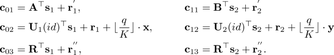
• Challenge ciphertext: when $\mathcal {A}$ submits a challenge $id^*$(distinct from all its queried id) and a pair of distinct message $(\mathbf {x}_0, \mathbf {y}_0)$ and $(\mathbf {x}_1, \mathbf {y}_1)$ which satisfies $\mathbf {x}^\top _0\mathbf {F}\mathbf {y}_0$ = $\mathbf {x}^\top _1\mathbf {F}\mathbf {y}_1$ for all queried $\mathbf {F}$, $\mathcal {B}$ picks $\beta \in \{0, 1\}$ and generates ciphertexts as follows:

  

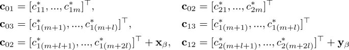
When $\mathcal {A}$ terminates with some output, $\mathcal {B}$ terminates with the same output.

It remains to analyze the reduction. It is easy to see that the master public key $\mathbf {A}, \mathbf {B}, \mathbf {R}$ and the random oracle responses $\mathbf {U}_{1}, \mathbf {U}_{2}$ are clearly uniformly random. Thanks to the discrete Gaussian distributions, for different $\mathbf {F}$, there are distinct $\mathbf {E}_{1}, \mathbf {E}_{2}$ which have enough entropy so that the adversary can not forge new $\mathbf {E}'_{1}, \mathbf {E}'_{2}$ corresponding to arbitrary $\mathbf {F}'$ and acquire more information than $\mathbf {x}^\top _{\beta }\mathbf {F}\mathbf {y}_{\beta }$ through collusion attacks. We claim that the probability that $\mathcal {B}$ does not abort during the simulation is $\frac{1}{Q_{\mathbf {U}_{1}, \mathbf {U}_{2}}}$ (this is proved by considering a game in which $\mathcal {B}$ can answer all secret key queries). We showed that if $\mathcal {B}$ does not abort during secret key queries, then the challenge ciphertexts is distributed as encryption of $\beta =0$ or $\beta =1$ depending on whether the LWE sample is real or random. Therefore, conditioned on $\mathcal {B}$ not aborting, $\mathcal {A}$’s view is statistically close to the one provided by the real IBFE CPA security experiment. Then, we have

$$\begin{aligned} Adv_{\mathcal {B}}^{{LWE}_{q, \chi _\alpha }} \ge \frac{Adv_{\mathcal {A}}^{IND-IBFE-CPA}}{Q_{\mathbf {U}_{1}, \mathbf {U}_{2}}}-negl(n). \end{aligned}$$

This concludes the proof. $\square$

6 Conclusions and Open Problems

We propose an adaptively secure IBFE scheme for quadratic functions from lattices in the random oracle model. Constructing adaptively secure FE scheme for quadratic functions under standard model is still an open problem.

We formalize the definitions of identity-based functional encryption (IBFE) and its indistinguishability security (IND-IBFE-CPA) which may apply to many scenarios and applications, and it seems easier to construct IBFE schemes than FE schemes, so we appeal for more constructions for more practical function classes for IBFE.

Lattice-based cryptography have many fascinating properties not found in other types of cryptography, but related techniques are still limited to construct and prove some primitives(e.g. FE), so whether we can construct an FE scheme for polynomial functions from standard assumptions is an appealing open problem.

References

Abdalla, M., Bourse, F., De Caro, A., Pointcheval, D.: Simple functional encryption schemes for inner products. In: Katz, J. (ed.) PKC 2015. LNCS, vol. 9020, pp. 733–751. Springer, Heidelberg (2015). https://doi.org/10.1007/978-3-662-46447-2_33
Agrawal, S., Boneh, D., Boyen, X.: Efficient lattice (H)IBE in the standard model. In: Gilbert, H. (ed.) EUROCRYPT 2010. LNCS, vol. 6110, pp. 553–572. Springer, Heidelberg (2010). https://doi.org/10.1007/978-3-642-13190-5_28
Agrawal, S., Freeman, D.M., Vaikuntanathan, V.: Functional encryption for inner product predicates from learning with errors. In: Lee, D.H., Wang, X. (eds.) ASIACRYPT 2011. LNCS, vol. 7073, pp. 21–40. Springer, Heidelberg (2011). https://doi.org/10.1007/978-3-642-25385-0_2
Agrawal, S., Libert, B., Stehlé, D.: Fully secure functional encryption for inner products, from standard assumptions. In: Robshaw, M., Katz, J. (eds.) CRYPTO 2016. LNCS, vol. 9816, pp. 333–362. Springer, Heidelberg (2016). https://doi.org/10.1007/978-3-662-53015-3_12
Agrawal, S., Rosen, A.: Functional encryption for bounded collusions, revisited. In: Kalai, Y., Reyzin, L. (eds.) TCC 2017. LNCS, vol. 10677, pp. 173–205. Springer, Cham (2017). https://doi.org/10.1007/978-3-319-70500-2_7
Ajtai, M.: Generating hard instances of the short basis problem. In: Wiedermann, J., van Emde Boas, P., Nielsen, M. (eds.) ICALP 1999. LNCS, vol. 1644, pp. 1–9. Springer, Heidelberg (1999). https://doi.org/10.1007/3-540-48523-6_1
Alwen, J., Peikert, C.: Generating shorter bases for hard random lattices. In: International Symposium on Theoretical Aspects of Computer Science, STACS 2009, pp. 75–86 (2009)
Ananth, P., Jain, A.: Indistinguishability obfuscation from compact functional encryption. In: Gennaro, R., Robshaw, M. (eds.) CRYPTO 2015. LNCS, vol. 9215, pp. 308–326. Springer, Heidelberg (2015). https://doi.org/10.1007/978-3-662-47989-6_15
Ananth, P., Sahai, A.: Functional encryption for turing machines. In: Kushilevitz, E., Malkin, T. (eds.) TCC 2016. LNCS, vol. 9562, pp. 125–153. Springer, Heidelberg (2016). https://doi.org/10.1007/978-3-662-49096-9_6
Baltico, C.E.Z., Catalano, D., Fiore, D., Gay, R.: Practical functional encryption for quadratic functions with applications to predicate encryption. In: Katz, J., Shacham, H. (eds.) CRYPTO 2017. LNCS, vol. 10401, pp. 67–98. Springer, Cham (2017). https://doi.org/10.1007/978-3-319-63688-7_3
Bethencourt, J., Sahai, A., Waters, B.: Ciphertext-policy attribute-based encryption. In: 2007 IEEE Symposium on Security and Privacy, pp. 321–334, May 2007
Bitansky, N., Nishimaki, R., Passelègue, A., Wichs, D.: From cryptomania to obfustopia through secret-key functional encryption. In: Hirt, M., Smith, A. (eds.) TCC 2016. LNCS, vol. 9986, pp. 391–418. Springer, Heidelberg (2016). https://doi.org/10.1007/978-3-662-53644-5_15
Bitansky, N., Vaikuntanathan, V.: Indistinguishability obfuscation from functional encryption. In: Proceedings of the 2015 IEEE 56th Annual Symposium on Foundations of Computer Science (FOCS), FOCS 2015, Washington, DC, USA, pp. 171–190(2015)
Boneh, D., Boyen, X.: Secure identity based encryption without random oracles. In: Franklin, M. (ed.) CRYPTO 2004. LNCS, vol. 3152, pp. 443–459. Springer, Heidelberg (2004). https://doi.org/10.1007/978-3-540-28628-8_27
Boneh, D., Franklin, M.: Identity-based encryption from the Weil pairing. In: Kilian, J. (ed.) CRYPTO 2001. LNCS, vol. 2139, pp. 213–229. Springer, Heidelberg (2001). https://doi.org/10.1007/3-540-44647-8_13
Boneh, D., et al.: Fully key-homomorphic encryption, arithmetic circuit ABE and compact garbled circuits. In: Nguyen, P.Q., Oswald, E. (eds.) EUROCRYPT 2014. LNCS, vol. 8441, pp. 533–556. Springer, Heidelberg (2014). https://doi.org/10.1007/978-3-642-55220-5_30
Boneh, D., Sahai, A., Waters, B.: Functional encryption: definitions and challenges. In: Ishai, Y. (ed.) TCC 2011. LNCS, vol. 6597, pp. 253–273. Springer, Heidelberg (2011). https://doi.org/10.1007/978-3-642-19571-6_16
Boneh, D., Waters, B.: Conjunctive, subset, and range queries on encrypted data. In: Vadhan, S.P. (ed.) TCC 2007. LNCS, vol. 4392, pp. 535–554. Springer, Heidelberg (2007). https://doi.org/10.1007/978-3-540-70936-7_29
Brakerski, Z., Langlois, A., Peikert, C., Regev, O., Stehlé, D.: Classical hardness of learning with errors. In: Proceedings of the Forty-fifth Annual ACM Symposium on Theory of Computing, STOC 2013, New York, NY, USA, pp. 575–584 (2013)
Cash, D., Hofheinz, D., Kiltz, E., Peikert, C.: Bonsai trees, or how to delegate a lattice basis. In: Gilbert, H. (ed.) EUROCRYPT 2010. LNCS, vol. 6110, pp. 523–552. Springer, Heidelberg (2010). https://doi.org/10.1007/978-3-642-13190-5_27
Cocks, C.: An identity based encryption scheme based on quadratic residues. In: Honary, B. (ed.) Cryptography and Coding 2001. LNCS, vol. 2260, pp. 360–363. Springer, Heidelberg (2001). https://doi.org/10.1007/3-540-45325-3_32
Coron, J.-S., Lee, M.S., Lepoint, T., Tibouchi, M.: Cryptanalysis of GGH15 multilinear maps. In: Robshaw, M., Katz, J. (eds.) CRYPTO 2016. LNCS, vol. 9815, pp. 607–628. Springer, Heidelberg (2016). https://doi.org/10.1007/978-3-662-53008-5_21
Garg, S., Gentry, C., Halevi, S.: Candidate multilinear maps from ideal lattices. In: Johansson, T., Nguyen, P.Q. (eds.) EUROCRYPT 2013. LNCS, vol. 7881, pp. 1–17. Springer, Heidelberg (2013). https://doi.org/10.1007/978-3-642-38348-9_1
Garg, S., Gentry, C., Halevi, S., Zhandry, M.: Functional encryption without obfuscation. In: Kushilevitz, E., Malkin, T. (eds.) TCC 2016. LNCS, vol. 9563, pp. 480–511. Springer, Heidelberg (2016). https://doi.org/10.1007/978-3-662-49099-0_18
Garg, S., Mahmoody, M., Mohammed, A.: When does functional encryption imply obfuscation? In: Kalai, Y., Reyzin, L. (eds.) TCC 2017. LNCS, vol. 10677, pp. 82–115. Springer, Cham (2017). https://doi.org/10.1007/978-3-319-70500-2_4
Garg, S., Gentry, C., Halevi, S., Raykova, M., Sahai, A., Waters, B.: Candidate indistinguishability obfuscation and functional encryption for all circuits. In: 2013 IEEE 54th Annual Symposium on Foundations of Computer Science(FOCS), pp. 40–49, October 2014
Gentry, C., Gorbunov, S., Halevi, S.: Graph-induced multilinear maps from lattices. In: Dodis, Y., Nielsen, J.B. (eds.) TCC 2015. LNCS, vol. 9015, pp. 498–527. Springer, Heidelberg (2015). https://doi.org/10.1007/978-3-662-46497-7_20
Gentry, C., Peikert, C., Vaikuntanathan, V.: Trapdoors for hard lattices and new cryptographic constructions. In: Proceedings of the Fortieth Annual ACM Symposium on Theory of Computing, STOC 2008, New York, USA, pp. 197–206 (2008)
Goldwasser, S., Kalai, Y., Popa, R.A., Vaikuntanathan, V., Zeldovich, N.: Reusable garbled circuits and succinct functional encryption. In: Proceedings of the Forty-fifth Annual ACM Symposium on Theory of Computing, STOC 2013, New York, NY, USA, pp. 555–564 (2013)
Gorbunov, S., Vaikuntanathan, V., Wee, H.: Functional encryption with bounded collusions via multi-party computation. In: Safavi-Naini, R., Canetti, R. (eds.) CRYPTO 2012. LNCS, vol. 7417, pp. 162–179. Springer, Heidelberg (2012). https://doi.org/10.1007/978-3-642-32009-5_11
Gorbunov, S., Vaikuntanathan, V., Wee, H.: Attribute-based encryption for circuits. In: Proceedings of the Forty-fifth Annual ACM Symposium on Theory of Computing, STOC 2013, New York, USA, pp. 545–554 (2013)
Gorbunov, S., Vaikuntanathan, V., Wee, H.: Predicate encryption for circuits from LWE. In: Gennaro, R., Robshaw, M. (eds.) CRYPTO 2015. LNCS, vol. 9216, pp. 503–523. Springer, Heidelberg (2015). https://doi.org/10.1007/978-3-662-48000-7_25
Goyal, V., Pandey, O., Sahai, A., Waters, B.: Attribute-based encryption for fine-grained access control of encrypted data. In: Proceedings of the 13th ACM Conference on Computer and Communications Security, CCS 2006, New York, USA, pp. 89–98 (2006)
Hu, Y., Jia, H.: Cryptanalysis of GGH map. In: Fischlin, M., Coron, J.-S. (eds.) EUROCRYPT 2016. LNCS, vol. 9665, pp. 537–565. Springer, Heidelberg (2016). https://doi.org/10.1007/978-3-662-49890-3_21
Katz, J., Sahai, A., Waters, B.: Predicate encryption supporting disjunctions, polynomial equations, and inner products. In: Smart, N. (ed.) EUROCRYPT 2008. LNCS, vol. 4965, pp. 146–162. Springer, Heidelberg (2008). https://doi.org/10.1007/978-3-540-78967-3_9
Lewko, A., Okamoto, T., Sahai, A., Takashima, K., Waters, B.: Fully Secure functional encryption: attribute-based encryption and (hierarchical) inner product encryption. In: Gilbert, H. (ed.) EUROCRYPT 2010. LNCS, vol. 6110, pp. 62–91. Springer, Heidelberg (2010). https://doi.org/10.1007/978-3-642-13190-5_4
Micciancio, D., Regev, O.: Worst-case to average-case reductions based on Gaussian measures. In: IEEE Symposium on Foundations of Computer Science, pp. 372–381 (2004)
Okamoto, T., Takashima, K.: Hierarchical predicate encryption for inner-products. In: Matsui, M. (ed.) ASIACRYPT 2009. LNCS, vol. 5912, pp. 214–231. Springer, Heidelberg (2009). https://doi.org/10.1007/978-3-642-10366-7_13
O’Neill, A.: Definitional issues in functional encryption. Cryptology ePrint Archive, report 2010/556 (2010). https://eprint.iacr.org/2010/556
Peikert, C.: Public-key cryptosystems from the worst-case shortest vector problem: extended abstract. In: Proceedings of the Forty-First Annual ACM Symposium on Theory of Computing, STOC 2009, New York, NY, USA, pp. 333–342 (2009)
Regev, O: On lattices, learning with errors, random linear codes, and cryptography. In: Proceedings of the Thirty-Seventh Annual ACM Symposium on Theory of Computing, STOC 2005, New York, NY, USA, pp. 84–93 (2005)
Sahai, A., Waters, B.: Fuzzy identity-based encryption. In: Cramer, R. (ed.) EUROCRYPT 2005. LNCS, vol. 3494, pp. 457–473. Springer, Heidelberg (2005). https://doi.org/10.1007/11426639_27
Sans, E.D., Pointcheval, D.: Unbounded inner product functional encryption, with succinct keys. Cryptology ePrint Archive, report 2018/487 (2018). https://eprint.iacr.org/2018/487
Shamir, A.: Identity-based cryptosystems and signature schemes. In: Blakley, G.R., Chaum, D. (eds.) CRYPTO 1984. LNCS, vol. 196, pp. 47–53. Springer, Heidelberg (1985). https://doi.org/10.1007/3-540-39568-7_5
Waters, B.: Functional encryption for regular languages. In: Safavi-Naini, R., Canetti, R. (eds.) CRYPTO 2012. LNCS, vol. 7417, pp. 218–235. Springer, Heidelberg (2012). https://doi.org/10.1007/978-3-642-32009-5_14
Waters, B.: A punctured programming approach to adaptively secure functional encryption. In: Gennaro, R., Robshaw, M. (eds.) CRYPTO 2015. LNCS, vol. 9216, pp. 678–697. Springer, Heidelberg (2015). https://doi.org/10.1007/978-3-662-48000-7_33
Author information
Authors and Affiliations
Corresponding author
Editor information
Editors and Affiliations
Rights and permissions
Copyright information
© 2018 Springer Nature Switzerland AG
About this paper
Cite this paper
Yun, K., Wang, X., Xue, R. (2018). Identity-Based Functional Encryption for Quadratic Functions from Lattices. In: Naccache, D., et al. Information and Communications Security. ICICS 2018. Lecture Notes in Computer Science(), vol 11149. Springer, Cham. https://doi.org/10.1007/978-3-030-01950-1_24
Download citation
DOI: https://doi.org/10.1007/978-3-030-01950-1_24
Published:
Publisher Name: Springer, Cham
Print ISBN: 978-3-030-01949-5
Online ISBN: 978-3-030-01950-1
eBook Packages: Computer ScienceComputer Science (R0)