
Abstract
In a Stroop task, participants can be presented with a color name printed in color and need to classify the print color while ignoring the word. The Stroop effect is typically calculated as the difference in mean response time (RT) between congruent (e.g., the word RED printed in red) and incongruent (GREEN in red) trials. Delta plots compare not just mean performance, but the entire RT distributions of congruent and incongruent conditions. However, both mean RT and delta plots have some limitations. Arm-reaching trajectories allow a more continuous measure for assessing the time course of the Stroop effect. We compared arm movements to congruent and incongruent stimuli in a standard Stroop task and a control task that encourages processing of each and every word. The Stroop effect emerged over time in the control task, but not in the standard Stroop, suggesting words may be processed differently in the two tasks.
Introduction
Participants in the Stroop task (Stroop 1935) are presented with a color-word printed in color and must respond to the color and ignore the word. They are faster, on average, to name the print color of a congruent color-word stimulus (e.g., the word RED printed in red) than an incongruent stimulus (e.g., GREEN in red). The Stroop effect is calculated as the difference in response time (RT) between congruent trials and incongruent trials, and demonstrates the unintended influence of the word. It is one of the most replicated experimental effects in cognitive psychology, yet despite years of research, there is no agreed theoretical resolution as to the cause of the effect (MacLeod 1991; Eidels et al. 2010; Eidels 2012).
Theoretical accounts of the Stroop effect (e.g., Palef & Olson, 1975; Logan, 1980; Cohen, Dunbar, & McClelland, 1990; Melara & Algom, 2003) must assume that participants process the meaning of the printed words despite instructions to ignore them and focus on the print color; otherwise the time to respond ‘red’ should be the same for any word printed in that color, regardless of whether it is congruent or incongruent—and hence, there would be no behavioral Stroop effect.
RTs have been the preferred dependent variable in many psychological experiments (see Luce, 1986), including the Stroop task. Researchers used RTs to determine that the Stroop effect is contingent on attentional resources (Kahneman and Chajczyk 1983), practice (MacLeod and Dunbar 1988), dimensional discriminability and experimental correlation (Dishon-Berkovits and Algom 2000), target set size (Heij and Vermeij 1987), and the number of colored letters in the stimulus word (Besner et al. 1997).
Despite their benefits, RTs provide only a single estimate of processing duration at the end of each trial, meaning there are limitations to what RTs can tell us about the time course of an experimental effect. For example, an RT of 500 ms on a given trial of the Stroop task suggests that it had taken 500 ms to perceptually encode a stimulus, process and decide on the color of the stimulus, and execute a behavioral response. However, we do not know how long each of these sub-processes takes.
There are statistical methods that provide insight into the time course of experimental effects. Parametric studies can fit sequential sampling models to RT distributions and estimate perceptual encoding time and rate of processing (e.g., Ratcliff & McKoon, 2008; S.D. Brown & Heathcote, 2008), but such models require strong assumptions and are therefore less general. Alternatively, graphical exploration methods of RT distributions, such as the delta plot, inform researchers about the time course of experimental effects with less assumptions (Jong et al. 1994).
Delta plots of Stroop data
Delta plots display graphically how an experimental effect changes across different points of two RT distributions. For instance, the left panel of Fig. 1 shows congruent and incongruent RT distributions of a hypothetical Stroop task. For delta plots, instead of calculating the Stroop effect as the difference between mean RTs of incongruent and congruent conditions, a researcher calculates the effect at a desired number of percentiles (e.g., at each decile of the two distributions). They could then plot the effect at each decile against the mean RT of the two distributions at each decile.Footnote 1 The resulting delta plot is shown in the right panel of Fig. 1. This function is always above 0, meaning that RTs in the incongruent distribution are slower than RTs in the congruent distribution for every decile. The positive slope suggests that the difference between the incongruent and congruent RTs is bigger for slower RTs than faster RTs.

The left panel depicts RT distributions for the congruent and incongruent conditions of a Stroop task. The right panel depicts the resulting delta plot
Pratte et al. (2010) used delta plots to investigate the distributional properties of the Stroop and Simon effects, and found delta plots with different slopes. Specifically, the slope for the Stroop effect delta function was positive, with small values for fast responses and larger values for slower responses. In contrast, the slope of the Simon effect delta function was negative, with large values for the fast responses and smaller values for slower responses. However, the delta plot slope depends on the exact nature of the task (cf. Proctor, Vu, & Nicoletti, 2003; Proctor & Shao, 2010; Dittrich, Kellen, & Stahl, 2014). The negative slope for the latter suggests that the Simon effect results from a conflict at the motor response stage, which decays over time. The positive slope for the Stroop effect delta function suggests the effect results from a conflict at the processing stage, which grows in magnitude as the participant processes the stimulus for a longer duration.
A potential limitation of the delta plot method is its sensitivity to the difference in variance between the distributions in question. This point is illustrated in Fig. 2, where we show delta plots that compare gamma distributions with different means and standard deviations (SD) to a gamma distribution with fixed arbitrary parameters—mean = 12 and SD = 3.Footnote 2 The middle panel serves as a benchmark and shows the delta plot of two identical gamma distributions with mean = 12 and SD = 3, resulting in a flat line at 0. Each column represents distributions with a different variance and each row represents distributions with a different mean. The effect of changes in variance on the slope of the delta plot, while the mean is held fixed, can be observed by moving along the columns within any given row. Critically, if one RT distribution had the same mean but larger variance than the other RT distribution, then the slope of the delta plot will be positive, regardless of the mean RT. Note that for empirical RT distributions, the standard deviation of RT typically increases linearly with the mean (Wagenmakers and Brown 2007), although there are cases where this trend does not hold, such as the Simon task (Pratte et al. 2010).

Simulated delta plots. Each delta plot is calculated by comparing gamma distributions with different means and SDs to a gamma distribution with mean = 12 and SD = 3. Each column shows a distribution with different SD and each row shows a distribution with different mean
There are limitations to investigating the time course of the Stroop effect using mean RTs, as they rely on a single measurement of latency at the end of each trial and ignore distributional information. The delta plot method makes use of the entire RT distribution, but effects of mean and variance are hard to discern (see Fig. 2). Moreover, RT distributions can have different shapes and be shifted in time. Ideally, researchers would like a measure that produces identically shaped distributions so that they can compare responses across the two distributions at the same points in time. We offer an alternative to the delta plot method, a method that allows researchers to look at experimental effects across identical distributions at the same points in time.
Reach-to-touch paradigm
A promising method in cognitive science is the reach-to-touch paradigm (Finkbeiner et al. 2014). For instance, in the Simon task literature, the reach-to-touch paradigm has already been used to investigate temporal properties of the effect (Porcu et al. 2016; Buetti and Kerzel 2010; Finkbeiner and Heathcote 2016). In a typical design, participants may be presented with a cognitive task that requires a speeded choice between two or more response alternatives. Participants execute their response by reaching out to designated spatial locations, say, left for color green and right for color red. The arm-movement trajectories are recorded and serve as the dependent measure.
There are two key components to the reach-to-touch paradigm. First, it is a continuous response measure that can reveal experimental effects as they emerge over time. Arm movements in the reach-to-touch paradigm have been considered a window into cognitive processes (Song and Nakayama 2009; Spivey et al. 2005). More recently, Finkbeiner and colleagues (Finkbeiner et al. 2014; Quek and Finkbeiner 2013; 2014) pointed out that this continuous response measure should be used with the second key component, the response signal procedure (Reed 1973; 1976).
The current study instructs participants to initiate their movement within 300 ms of an imperative ‘go’ signal. This go signal is the final beep in a sequence of three beeps. Importantly, on each trial, the three beeps occur randomly, so that the final ‘go’ beep appears at different points in time relative to the onset of the target stimulus. The time at which the participant begins moving relative to stimulus onset is the movement initiation time (MIT). For example, MIT = 0 means that the subject started to move their finger at the same time as the stimulus was presented. Similarly, MIT = 300 indicates that the subject lifted their finger from the start point 300 ms after the stimulus onset. A negative MIT means that the subject starting moving their finger before having seen the stimulus. MITs represent movements that commence at a range of different stimulus processing times. In the Stroop milieu, we can examine the magnitude of the Stroop effect for various processing times (i.e., is the observed effect larger on late lift-off trials, which presumably allow more time for processing).
The forced-reading Stroop task
As well as the statistical methods discussed, recent experimental methods have shed light on the nature of the Stroop effect. Eidels et al. (2014) employed a novel forced-reading Stroop task and found the standard Stroop effect is only a proportion of the Stroop effect that could be observed. In the standard task, participants are asked to classify the print color of color-words irrespective of the content of the word. In the forced-reading task, participants were asked to classify the print color of color-words (e.g., RED, GREEN), but withhold their response when presented with non-color-words (BED, GREED). To conform with the instructions, participants were forced to read every word presented. Consequently, the forced-reading Stroop task yielded a Stroop effect derived from fully processed words on every trial. Eidels et al. found a larger Stroop effect in the benchmark forced-reading task compared to the standard Stroop task, and suggested that the nature of reading occurring in the two tasks is not comparable.
The current study
In the present study, we use both the standard and forced-reading Stroop tasks in conjunction with measurements of arm-reaching trajectories to understand the time course of the Stroop effect.Footnote 3 The forced reading task is a useful benchmark, as it yields a Stroop effect from fully processed words.
The key aspect of our study is that distributions of MITs do not differ across conditions in our experiment (see Fig. 3). There were no differences in the means or the SDs of how long subjects view and presumably process the stimulus before initiating their movement. Therefore, we compared arm reaching trajectories across two identically shaped Stroop distributions to see if the Stroop effect unfolds at a different rate, for the standard and forced task, at the same points in time. Our analysis is not compromised by differences in variances or shapes between the congruent and incongruent distributions, thus our study addresses concerns with the delta plot.

Distribution of MITs for congruent and incongruent conditions in the standard and forced Stroop tasks. The four MIT distributions of interest do not differ in location or scale. Zero value on the x-axis means that the participant initiated movement at the same time as the stimulus onset. The figure shows that the majority of responses were initiated after stimulus onset. In the standard task, the mean MIT was 172 ms in the congruent condition and 169 ms in the incongruent condition. In the forced task, the mean MIT was 166 ms in both the congruent and incongruent conditions
We address four key research questions in our study. First, we expect that participants will be more informed of the correct response with additional processing time. So, do participants get a better idea of how to respond at later MITs? Second, there is an increased task demand in the forced-reading Stroop task because participants are required to read each and every word, but does this task demand result in the decision process unfolding faster in the standard Stroop task compared to the forced-reading Stroop task? Third, researchers have inferred from delta plots that Stroop interference grows over time (Pratte et al. 2010). This conclusion is also in line with extant theories of the Stroop effect (Cohen et al. 1990; Melara and Algom 2003). However, given the limitations of the delta plot, we investigate whether the Stroop effect (when it exists) grows over time in the reach-to-touch paradigm. Finally, the standard Stroop has previously been found to be a proportion of the benchmark forced-reading Stroop effect (Eidels et al. 2014). With our method we look at whether the Stroop effect grows in magnitude in the forced-reading task more than the standard Stroop task as stimulus-processing/viewing time increases.
Method
Participants
Twenty psychology students from Macquarie University participated in the study in return for course credit. All participants were native English speakers with normal or corrected-to-normal vision, intact color vision, and reported to be right-handed. All participants took part in both the standard and forced-reading Stroop tasks.
Apparatus
A schematic of the experimental apparatus is presented in Fig. 4, with important materials labeled with numbers. Participants sat in front of a table and placed their right index finger on a small Velcro square (marked ‘0’ in Fig. 4), which marks the starting position and the return position for every trial. Stimuli were presented on a 27” Samsung LCD/LED monitor using the software ‘Presentation’. The monitor was situated 1 m away from the participants and centered with their body mid-line. Lateral response boards (30 cm x 9 cm) were placed to the left (1) and right (2) of the monitor, 75 cm apart and 50 cm from the front of the desk. A third response location (3) was marked on the desk between the participant and the monitor, 50 cm away from the front edge of the desk. A small motion-tracking sensor was taped to the tip of the right index fingertip of each participant. A Polhemus Liberty (240 Hz) electromagnetic motion tracking system was used to record the participants arm trajectories during the experiment. Participants wore headphones adjusted to a comfortable volume level, which were used to present a sequence of beeps.

A front-facing view of the apparatus used for the current experiment. Subjects placed their index finger on position 0 to start the trial. On each trial, participants reached toward the color response options, denoted by 1 and 2. In the forced-reading task, participants could also reach towards a neutral response option, denoted by 3
Stimuli
The standard Stroop task and the forced-reading Stroop task used the same stimuli. The stimuli were the color-words: RED and GREEN; and the non-color-words were: ROD, BED, RENT, QUEEN, GRAIN, and GREED. These non-color stimuli were specifically selected to ensure that participants would not base their responses on local cues. The non-color stimuli were the orthographic neighbors of the color-words with the closest frequency, such that each non-color-word shared all but one or two letters with a color-word (see Eidels et al., 2014). All words were printed in either the color red or green (with RGB values of 220/0/0 and 0/170/0, respectively) and were written in uppercase Garamond font, which at a viewing distance of 1 m allowed for a visual angle of 4 degrees. Each of the color-words could be congruent to the font color (e.g., RED printed in the color red) or incongruent (e.g., RED printed in the color green). All non-color words can be considered neutral to the font color, whether they were printed in red or green (but see T. L. Brown, 2011).
Design and procedure
Each participant attended two experimental sessions: the standard Stroop task and the forced-reading Stroop task. Sessions were separated by a minimum of 1 day and a maximum of 7 days. The order of task administration was counterbalanced across participants so that half of the participants performed the standard Stroop task first, and the remaining half performed the forced-reading Stroop task first. The order of word presentation was random for each participant. For each session, the participant performed in 840 trials. These trials were partitioned into seven blocks of 120 trials each. There were 2-min breaks between each block administration. In each block, color-words were presented 15 times per combination of color × word (RED in red, RED in green, GREEN in red, and GREEN in green), which made for 60 color-word trials. The six non-color words were presented five times per combination, making for 60 non-color word trials within the same block.
In the standard Stroop task, the participant classified the color of all the words presented by reaching out to the left or right lateral response boards (‘1’ and ‘2’ in Fig. 4). The left and right response boards corresponded to a red or a green color and were counter balanced across participants. In the forced-reading Stroop task, participants classified the color of color-words but did not classify the color of non-color words. For non-color words, participants responded by reaching towards a neutral response location (‘3’ in Fig. 4).
On each trial, a single word in color was presented at the center of a black screen. The timing of stimulus presentation was relative to the sound of three auditory beeps that were played through the participant’s headphones. The stimulus was randomly presented, with equal probability, at one of five different times prior to the third beep (300, 230, 150, 70, or 0 ms before the third beep). In four of the five timing conditions (i.e., 80% of trials), the stimulus was presented before the onset of the third beep, whereas in the 0-ms condition (20% of trials) the stimulus and the third beep were presented simultaneously. This procedure controls for participant’s anticipation of stimulus display. In both tasks, participants had to initiate their movement between 100 ms before and 200 ms after the third beep, meaning all movement begun within a 300-ms window around the third beep. Two example trial sequences are presented in Fig. 5. If participants failed to initiate movement within the allotted time-window, they would receive a loud buzzing sound and visual feedback to indicate they had responded ‘Too Early!’ or ‘Too Late!’. Once a movement was initiated, participants were required to maintain a continuous forward motion. Failing to do so terminated the trial and participants were provided with a buzz and appropriate visual feedback. Trials that were terminated via movement errors were repeated at a later stage of the block. The presentation of the trial terminated when the participant responded via the response points. The next trial followed after the sensor was returned to the start point.

Example trial sequences for trials in which stimuli were presented simultaneously with the third beep (top panel; 0-ms gap between the onset of the stimulus and the third beep) and 300 ms before the third beep (bottom). The red vertical bars below the time line indicate the onset of the three auditory beeps, the green bar above the time line indicates stimulus onset, and the blue box shows the 300-ms window in which participants begun their movements. In addition to the 0- and 300-ms trial types, there were also trials in which stimulus onset preceded the third beep by 70, 150, or 230 ms (not shown in the figure)
Data analysis
From the trajectories (Fig. 6), we calculated the velocity along the x-axis (x-velocity), which serves as our dependent measure. X-velocity quantifies how fast a participant is moving in the correct direction at any time during the trial. X-velocity is positive for movements towards the correct direction and negative for movements toward the incorrect direction. Thus, x-velocity provides data that ranges between fast movement in the correct direction (large positive values) and fast movement in the incorrect direction (large negative values). It is a more informative measure compared to nominal accuracy rates (correct/incorrect) or RTs, which range from ‘slow’ to ‘fast’ in only a positive direction.

Arm trajectories and mean arm trajectories of a single participant. The four panels include arm trajectories related to the four possible conditions obtained from crossing Task by Congruence. X and Y labels refer to the movement planes presented in Fig. 4. The Y-axis denotes forward motion and the X-axis denotes lateral motion. Trajectories only include correct responses. Thus, any differences between the left and right tracks are natural deviations in how the hand moves to a target situated to the left versus right of mid-line
Before calculating x-velocity, the positional data taken from the Polhemus Liberty device was filtered with a two-way low-pass Butterworth filter at 7 Hz, which reduced noise in the data. Then, x-velocity was derived from the numerical differentiation of the filtered positional data. The onset of movement was identified as the first of 20 consecutive samples in which the tangential velocity exceeded 10 cms/s. The offset of movement was identified as the first of 20 consecutive samples of tangential velocity that occurred after peak velocity and that were less than 10 cms/s.
For our analysis, we first improved the signal-to-noise ratio of the trajectories with a modified version of orthogonal polynomial trend analysis (OPTA). The OPTA procedure used here has been described in detail in Finkbeiner et al. (2014) and Finkbeiner and Heathcote (2016). In summary, OPTA uses a regression model with x-velocity as the dependent variable and MIT (with polynomial terms up to the 15 th order) as the predictor variable. Terms that did not explain significant variance were removed from the model, leaving only significant coefficients to predict x-velocity for each trial. After the OPTA analysis, we calculated the mean predicted x-velocity values from the first 350 ms of the reaching movement (initial x-velocity; Finkbeiner et al., 2014). We limit our dependent measure to the first 350 ms because the initial part of the trajectory represents the motor plan participants had formulated just prior to initiating their movement. The MIT latencies were used to group the initial x-velocity profiles into 20 equal bins (i.e., semi-deciles). Finally, the mean predicted initial x-velocity values were then subjected to a linear mixed-effects model with MIT semi-decile included as a fixed effect.
Results
Accuracy
Overall, across all participants, 91% of the responses were correct and valid. Mean error rate amounted to a negligible 1%. Invalid responses consisted of responding too early (3%), responding too late (5%), and not moving fast enough (2%). None of the participants were excluded from analysis due to accuracy.
Linear-mixed effects analysis
The linear mixed-effects analysis on predicted initial x-velocity (x-velocity hereafter) was conducted only for correct responses. We used a model comparison approach with the Bayesian information criterion (BIC Schwarz, 1978), which selects the best-fitting model while penalizing for complexity (i.e., number of parameters). The best-fitting model included task (forced, standard), condition (congruent, incongruent), and MIT (semidecile) as fixed effects. The model also included subjects as a random effect. The relationship between x-velocity and MIT was curvilinear and so the model included up to 3rd order terms for MIT. Here we report the coefficients (b), standard errors, and t-values of the best-fitting model. The criterion for significance is a coefficient magnitude of at least twice the corresponding standard error. For the ‘condition’ factor, the congruent condition was used as a baseline meaning that negative coefficients represent smaller x-velocities relative to the congruent condition. For the ‘task’ factor, the standard task was used as a baseline, meaning that negative coefficients represent smaller x-velocities relative to the standard task.
X-velocity was smaller in the forced Stroop task compared to the standard task (b=−34.80, SE = 0.32, t=−109.32). There was also a smaller x-velocity in the incongruent condition compared to the congruent condition (b=− 4.07, SE = 0.32, t=−12.87). X-velocity increased as a function of MIT semidecile (b=1606.03, SE = 21.07, t= 76.21). There was a significant interaction between task and condition, where the difference in x-velocity between congruent and incongruent trials was bigger in the forced task than the standard task (b=−2.76, SE = 0.46, t=−6.05). There was an interaction between task and MIT semidecile (b=−825.75, SE = 30.10, t=−27.43), but no interaction between condition and MIT semidecile (b=59.50, SE = 29.85, t=1.99). Finally, there was a three-way interaction between task, condition, and MIT semidecile (b=−665.88, SE = 43.08, t=−15.46).
To understand the nature of the three-way interaction we ran paired t-tests (congruent vs. incongruent) at each of the 20 MIT semideciles for both the standard Stroop task and the forced Stroop task (Fig. 7). We corrected for an inflated type I error rate with Bonferroni corrected p values. This analysis showed the Stroop effect unfolding over time. In the standard task, the Stroop effect was not significant for any of the 20 MIT semideciles.Footnote 4 However, in the forced task, the Stroop effect was significant for movements that commenced at the 7th MIT semidecile (∼ 133ms) through to the 20th and final MIT semidecile (∼ 338ms).
Discussion
Participants performed in both a standard and forced-reading Stroop task. The dependent measure for both tasks were the reaching trajectories. Using arm-reaching trajectories coupled with a signal-to-respond procedure allowed us to compare Stroop effects that are calculated from two identically shaped distributions. This way, we could compare Stroop effects at the same points in time and presumably equivalent processing times. At each point in time we observed how fast the participant initially moved towards the correct response—initial x-velocity.
First, we wanted to know if participants get a better idea of how to respond with increased stimulus processing/viewing time (processing time for brevity). Initial x-velocity significantly increased as a function of MIT. Thus, the participant moved faster toward the correct response when they had more processing time. This finding might not be surprising, as the participant would be more informed of the correct response with additional time. Nonetheless, this finding supports our claim that the impact of increased processing time can manifest in our initial x-velocity-dependent measure.
Second, we looked at whether their was a difference in overall performance in the forced-reading Stroop task compared to standard Stroop task, as the forced task had a greater task demand. We found that initial x-velocity increased more quickly as a function of MIT for the standard task than the forced task. This suggests that the participant’s decision process unfolded at a faster rate over time in the standard task compared to the forced task.
Finally, we wanted to know if the Stroop magnitude emerged with more processing time and if the effect grew in the forced-reading task more than the standard Stroop task. We found that the Stroop effect was not evident in neither the standard nor forced tasks prior to approximately 133 ms of processing time. Yet, after 133 ms, the Stroop effect was only evident in the forced task and not the standard task. In the forced task, the Stroop effect continued to grow in magnitude after 133 ms. The lack of effect in the standard task suggests the standard Stroop effect is only a proportion of the benchmark forced-reading Stroop effect. Crucially, this finding does not depend on the amount of processing time—although some processing time, namely 133 ms, is needed for significant differences between the standard and forced-reading Stroop task to emerge.
Validating findings from delta plots and forced-reading
Pratte et al. (2010) advocated the delta plot as a method for examining the time course of experimental effects, such as the Stroop effect. In their application of the delta function, they found that the Stroop effect was small for fast responses and large for slow responses. Their finding suggested that the effect grows in magnitude as processing time increased, but the slope of the delta plot is sensitive to the variance of the distributions in question, limiting its applicability. We showed that when the Stroop effect is observed, it grows in magnitude as the processing time increases, even when assessed without the confounds of delta plots.
However, a significant Stroop effect only emerged in the forced Stroop task. The lack of a Stroop effect in the standard task is not a surprising result. Despite the reputation of the Stroop effect as a robust phenomenon, it has been shown to depend on design as well as other contextual factors. The effect appears only when certain conditions are met, but can be very small and even reversed given particular contextual factors (e.g., Kahneman & Chajczyk, 1983; MacLeod & Dunbar, 1988; Dishon-Berkovits & Algom, 2000; Besner et al., 1997; La Heij & Vermeij, 1987). In his comprehensive review of Stroop research, MacLeod (1991) listed set-size, mode of response, and relative speed of processing (among other factors) as factors that determine the magnitude of the effect. Since MacLeod, a substantial number of empirical papers have shown the malleable nature of the Stroop effect and how, with small set size and manual responses, it can be quite small and even vanish (see, e.g., Melara & Mounts, 1993; Dishon-Berkovits & Algom, 2000; Sabri, Melara, & Algom, 2001; Melara & Algom, 2003).
Our experimental design was limited to only two colors and to a manual (rather than vocal) mode of response, both known to limit the magnitude of the Stroop effect (see also Eidels et al., 2010). Nonetheless, a marked Stroop effect was registered in the forced-reading task of the current study, suggesting that the effect can emerge even with two colors and a manual mode of responding. Its absence in the standard task does not merely reflect sensitivity to set size or to the mode of responding, but rather suggests that words in the standard Stroop task may not be fully processed, at least not to the same extent they are processed in the forced task.
The asymmetry in Stroop effects across the standard and forced tasks could potentially be explained by the complexity of the forced-reading task. Specifically, Eidels et al. (2014) documented longer response times in the forced task, with the additional time allowing for the irrelevant word to interfere with color naming more (e.g., Melara and Algom, 2003).
The present study offers another way to expand on the findings of Eidels et al. (2014) by providing the means to directly examine the magnitude of the Stroop effect at the same points in processing time across the two tasks. Participants in the present study initiated their reaching responses in synchrony with an imperative go signal, as opposed to the target stimulus. Thus, we were able to equate the movement initiation times across the two tasks, despite the differences in task difficulty/complexity. When we compared the magnitude of the Stroop effect across tasks at similar points in stimulus-processing time, we observe a clear Stroop effect in the forced-reading version of the task at all time points greater than 133 ms. In contrast, the magnitude of the effect is reduced at the corresponding time points in the standard version of the task. Expanding on Eidels et al. (2014) we show that the larger Stroop effect under forced-reading instructions is not an artifact due to longer processing time, but a genuine effect.
Theoretical implications
A central result of the current study is the larger difference observed between the incongruent and congruent conditions (i.e., larger Stroop effect) at longer movement initiation times (see Fig. 7) in the forced reading task. Existing theories of the Stroop effect may differ in their predictions concerning the magnitude of the effect as processing time increases. We briefly survey three popular models and discuss whether they can predict this observed result.
The horse race model of the Stroop effect (Palef and Olson 1975) suggests that activation of the word and color information accumulates in parallel. Word and color information accumulate toward a response channel, where task irrelevant word information arrives first. Because the word channel finishes first our cognitive system needs to wait for a response activated by the slower color information, which manifests as Stroop interference. This model has been criticized as it cannot account for data where the word information is delayed (e.g., Glaser & Glaser, 1982). In regards to our study, the horse race account cannot accommodate a Stroop effect that grows over time, which we observed in the forced reading task.
A current and popular account of the Stroop task is the parallel distributed processing model (Cohen et al. 1990). This model suggests that our system receives information (input) from different dimensions that travel down specific pathways to response mechanisms (output). Some of these pathways have stronger activation than others and the strength of this activation, not the speed, determines the output. In the Stroop task, the word pathway is considered stronger than the color pathway. Because word processing is more likely to reach the output node before color processing, additional activation needs to be recruited from task-specific nodes, which cause the system to run for many more processing cycles.Footnote 5 This account is in line with our results as longer processing times produce greater Stroop interference.
Similarly, our results are in line with the tectonic theory of selective attention (Melara and Algom 2003). In this model, evidence from target relevant information lead to the response required on the trial and values of the non-presented target lead to an incorrect response. A ratio of this evidence is calculated, and once the ratio reaches 1, a response is made. When there is more evidence for the non-presented target (i.e., when you have processed the word for longer) than the presented target, more processing steps are required to exceed the response threshold.
The fact that we found a Stroop effect in the forced task, but not the standard, sheds light on the nature of reading in the Stroop task. For instance, on any particular trial of the standard task, a participant might be processing the word to some extent or not reading the word at all. Eidels et al. (2014) posit a simple probability-mixture model to account for these results. Under this model, the empirical congruent and incongruent distributions we observe are binary mixtures of two unobserved distributions. A given trial is a sample drawn from the distribution associated with reading (with probability p) or the distribution free of word reading (with probability 1-p). The forced reading task increases the probability of reading to (p = 1). This should lead to an inflated Stroop effect compared with the standard task, which is what we observe in our data.
Conclusions
Our study has methodological and theoretical implications. The arm reaching paradigm can potentially reveal how experimental effects emerge over time. We found that when the Stroop effect is observed, it grows in magnitude with more time for processing—and this finding was demonstrated without the confounds of delta plots. We also showed that the nature of reading in the standard Stroop task is not comparable to a task in which we know the participant reads on every trial.
Notes
The benefit of plotting percentile effects as a function of percentile means is that the delta plot will be linear (Speckman et al. 2008).
Typically the gamma distribution is parameterized with the shape and rate parameter. Given that the mean of the gamma distribution \(= \frac {shape}{rate}\) and the SD of the gamma distribution \(= \frac {\sqrt {shape}}{rate}\), the shape and rate parameters we used to generate data were shape \(= \frac {mean^{2}}{SD^{2}}\) and rate \(= \frac {mean}{SD^{2}}\) (e.g., Kruschke, 2011, p. 170).
The term ‘standard Stroop task’ is a neutral term we use to refer to a Stroop task in which participants are not ensured to read on each and every trial. Standard Stroop tasks typically use response time as the dependent measure, have a vocal mode of responding, and have more than two color stimuli (but see MacLeod, 1991).
We ran 20 Bonferroni corrected t-tests across the semi-deciles separately for the two different sessions. We found that the results of the standard Stroop effect were not dependent on the session order as no standard Stroop was found for either session.
Fig. 7 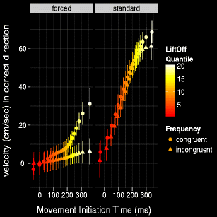
Initial x-velocity by MIT and Condition (congruent and incongruent) in standard and forced Stroop task. Error bars represent within-subjects 95% CIs. MIT values indicate the time delay between stimulus onset and the beginning of the response movement. The Stroop effect is represented by the vertical difference in height between the congruent (circles) and incongruent (triangles) markers at each quantile. Stroop effect is null on early quantiles of the forced task, but emerges later on. It is effectively null in the standard task, for all quantiles
See Botvinick et al. (2001), who expanded the parallel distributed processing model to explain how our cognitive system monitors and regulates conflict.

References
Besner, D., Stolz, J. A., & Boutilier, C. (1997). The Stroop effect and the myth of automaticity. Psychonomic Bulletin & Review, 4(2), 221–225.
Botvinick, M. M., Braver, T. S., Barch, D. M, Carter, C. S, & Cohen, JD (2001). Evaluating the demand for control: anterior cingulate cortex and conflict monitoring. Psychological Review, 108, 624–652.
Brown, T. L. (2011). The relationship between Stroop interference and facilitation effects: statistical artifacts, baselines, and a reassessment. Journal of Experimental Psychology: Human Perception and Performance, 37(1), 85–99.
Brown, S. D., & Heathcote, A. (2008). The simplest complete model of choice response time: linear ballistic accumulation. Cognitive Psychology, 57(3), 153–178.
Buetti, S., & Kerzel, D. (2010). Effects of saccades and response type on the Simon effect: if you look at the stimulus, the Simon effect may be gone. The Quarterly Journal of Experimental Psychology, 63(11), 2172–2189.
Cohen, J. D., Dunbar, K., & McClelland, J. L (1990). On the control of automatic processes: a parallel distributed processing account of the Stroop effect. Psychological Review, 97(3), 332–361.
Dishon-Berkovits, M., & Algom, D. (2000). The Stroop effect: it is not the robust phenomenon that you have thought it to be. Memory & Cognition, 28(8), 1437–1449.
Dittrich, K., Kellen, D., & Stahl, C. (2014). Analyzing distributional properties of interference effects across modalities: chances and challenges. Psychological Research, 78(3), 387–399.
Eidels, A. (2012). Independent race of colour and word can predict the Stroop effect. Australian Journal of Psychology, 64(4), 189–198.
Eidels, A., Townsend, J. T., & Algom, D. (2010). Comparing perception of Stroop stimuli in focused versus divided attention paradigms: evidence for dramatic processing differences. Cognition, 114(2), 129–150.
Eidels, A., Ryan, K., Williams, P., & Algom, D. (2014). Depth of processing in the Stroop task: evidence from a novel forced-reading condition. Experimental Psychology, 61(5), 385–393.
Finkbeiner, M., & Heathcote, A. (2016). Distinguishing the time-and magnitude-difference accounts of the Simon effect: evidence from the reach-to-touch paradigm. Attention, Perception, & Psychophysics, 78(3), 848–867.
Finkbeiner, M., Coltheart, M., & Coltheart, V. (2014). Pointing the way to new constraints on the dynamical claims of computational models. Journal of Experimental Psychology: Human Perception and Performance, 40(1), 172–85.
Glaser, M. O., & Glaser, W. R. (1982). Time course analysis of the Stroop phenomenon. Journal of Experimental Psychology: Human Perception and Performance, 8(6), 875–894.
Heij, W. L., & Vermeij, M. (1987). Reading versus naming: the effect of target set size on contextual interference and facilitation. Perception & Psychophysics, 41(4), 355–366.
Jong, R. D., Liang, C. -C., & Lauber, E. (1994). Conditional and unconditional automaticity: a dual-process model of effects of spatial stimulus-response correspondence. Journal of Experimental Psychology: Human Perception and Performance, 20(4), 731–750.
Kahneman, D., & Chajczyk, D. (1983). Tests of the automaticity of reading: dilution of Stroop effects by color-irrelevant stimuli. Journal of Experimental Psychology: Human Perception and Performance, 9(4), 497–509.
Kruschke, J. K. (2011). Doing Bayesian analysis: A tutorial with R and BUGS. Academic Press.
Logan, G. D. (1980). Attention and automaticity in Stroop and priming tasks: theory and data. Cognitive Psychology, 12(4), 523–553.
Luce, R. D. (1986). Response times: Their role in inferring elementary mental organization (Number 8). Oxford University Press.
MacLeod, C. (1991). Half a century of research on the Stroop effect: an integrative review. Psychological Bulletin, 109, 163–203.
MacLeod, C., & Dunbar, K. (1988). Training and Stroop-like interference: evidence for a continuum of automaticity. Journal of Experimental Psychology: Learning, Memory, and Cognition, 14(1), 126–135.
Melara, R. D., & Algom, D. (2003). Driven by information: a tectonic theory of Stroop effects. Psychological Review, 110(3), 422–471.
Melara, R. D., & Mounts, J. R. W. (1993). Selective attention to Stroop dimensions: effects of baseline discriminability, response mode, and practice. Memory & Cognition, 21(5), 627–645.
Palef, S. R., & Olson, D. R. (1975). Spatial and verbal rivalry in a Stroop-like task. Canadian Journal of Psychology/Revue canadienne de psychologie, 29(3), 201–209.
Pratte, M. S., Rouder, J. N., Morey, R. D., & Feng, C. (2010). Exploring the differences in distributional properties between Stroop and Simon effects using delta plots. Attention, Perception, & Psychophysics, 72(7), 2013–25.
Proctor, R. W., Kim-Phuong, L V., & Nicoletti, R. (2003). Does right-left prevalence occur for the Simon effect? Perception & Psychophysics, 65(8), 1318–1329.
Proctor, R. W., & Shao, Chunhong (2010). Does the contribution of stimulus-hand correspondence to the auditory Simon effect increase with practice? Experimental Brain Research, 204(1), 131–137.
Porcu, E., Bölling, L., Lappe, M., & Liepelt, R. (2016). Pointing out mechanisms underlying joint action. Attention, Perception, & Psychophysics, 1–6.
Quek, G. L., & Finkbeiner, M. (2013). Spatial and temporal attention modulate the early stages of face processing: behavioural evidence from a reaching paradigm. PLoS One, 8(2), 57365–57365.
Quek, G. L., & Finkbeiner, M. (2014). Face-perception is superior in the upper visual field: evidence from masked priming. Visual Cognition, 22(8), 1038–1042.
Ratcliff, R., & McKoon, G. M. (2008). The diffusion decision model: theory and data for two-choice decision tasks. Neural Computation, 20, 873–922.
Reed, A. V. (1973). Speed-accuracy trade-off in recognition memory. Science, 181(4099), 574–576.
Reed, A. V. (1976). List length and the time course of recognition in immediate memory. Memory & Cognition, 4(1), 16–30.
Stroop, R. J. (1935). Studies of interference in serial verbal reactions. Journal of Experimental Psychology, 18 (6), 643–662.
Sabri, M., Melara, R. D., & Algom, D. (2001). A confluence of contexts: asymmetric versus global failures of selective attention to Stroop dimensions. Journal of Experimental Psychology: Human Perception and Performance, 27(3), 515–537.
Schwarz, G. (1978). Estimating the dimension of a model. The Annals of Statistics, 6(2), 461–464.
Speckman, P. L., Rouder, J.N., Morey, R.D., & Pratte, M.S. (2008). Delta plots and coherent distribution ordering. The American Statistician, 62, 262–266.
Spivey, M. J., Grosjean, M., & Knoblich, G. (2005). Continuous attraction toward phonological competitors. Proceedings of the National Academy of Sciences of the United States of America, 102(29), 10393–10398.
Song, J. -H., & Nakayama, K. (2009). Hidden cognitive states revealed in choice reaching tasks. Trends Cognition Science, 13(8), 360– 6.
Wagenmakers, E.-J., & Brown, S. (2007). On the linear relation between the mean and the standard deviation of a response time distribution. Psychological Review, 114(3), 830–841.
Author information
Authors and Affiliations
Corresponding author
Additional information
Author Note
This work was supported in part by an Australian Research Fellowship (FT120100830) to Matthew Finkbeiner from the Australian Research Council. We would like to thank Todd Kahan, Michael Masson, and Kerstin Dittrich for their constructive and detailed comments. We would also like to thank Brenda Ocampo for organizing and collecting data.
Rights and permissions
About this article

Cite this article
Tillman, G., Eidels, A. & Finkbeiner, M. A reach-to-touch investigation on the nature of reading in the Stroop task. Atten Percept Psychophys 78, 2547–2557 (2016). https://doi.org/10.3758/s13414-016-1190-8
Published:
Issue Date:
DOI: https://doi.org/10.3758/s13414-016-1190-8