
Abstract
More and more studies are based on digital microstructures of cement pastes obtained either by numerical modelling or by experiments. A comprehensive understanding of the their pore structures, therefore, becomes significant. In this study, the pore structure of a virtual cement paste (HYMO-1d) generated by cement hydration model HYMOSTRUC 3D is characterized. The pore structure of HYMO-1d is compared to the one of CT-1d that is reconstructed by using X-ray computed tomography technique (CT scan). Both HYMO-1d and CT-1d have the same porosity. Various parameters are taken into account, viz., the specific surface area, the pore size distribution (PSD), the connectivity and the tortuosity of water-filled pores. Regarding the PSD, two concepts (i.e., the “continuous PSD” and the “PSD by MIP simulation”) are adopted. The “continuous PSD” is believed to be a “realistic” PSD; while the “PSD by MIP simulation” is affected by the “throat” and “ink bottle” pores. The results show that HYMO-1d and CT-1d exhibit a similar curve of “continuous PSD”, but distinct curves of “PSD by MIP simulation” and different specific surface areas. A lower complexity of the pore structure of HYMO-1d is indicated by a higher tortuosity of water-filled pores with reference to CT-1d. This study indicates that the comparison of pore structures between the digital microstructures should be based on multiple parameters. It also gives an insight into further studies on digital microstructures, i.e. transport properties of unsaturated materials.
1 General introduction
The topology of the pore structure is a crucial property with respect to the hydraulic behaviour and ionic diffusion in porous media [1]. The durability of a porous material is highly dependent on its pore structure and the moisture state [2]. Based on the pore structure of a cementitious material, water distribution is found to have a significant influence on the durability of cementitious materials in terms of chemical ingress [3]. The diffusivity of ions varies a lot for a material with different water saturations, because a continuous water phase is more likely to form in the pore space at higher water saturations, and provides a path for ingressive ions, e.g. chloride and sulphate, etc. [4].
In cementitious materials, pores can be simply classified into two groups, namely capillary pores (pore size/diameter d > 10 nm) and gel pores (d < 10 nm), while large capillary pores have a size 50 nm < d < 10 μm [5]. To characterize the pore structure, mercury intrusion porosimetry (MIP) has been widely used, by which a wide range of pore size distribution (PSD) from nanometre to microns can be determined [6]. In this technique, mercury as a non-wetting liquid is intruded into a porous material at a progressively increased pressure P. The pore size d can be determined based on the well-known Washburn equation: d = −4 g cos θ/P, where g is the surface tension of mercury, θ is the contact angle of mercury on the solid. However, due to “throat” and “ink bottle” effects, MIP measurements systematically misallocate the sizes of almost all pores in hydrated cementitious materials, and assign to sizes smaller than the actual ones [7]. This misallocation has been confirmed by observation of samples intruded by Wood’s metal [8]. To alleviate the underestimation of large pores by MIP measurement, a step by step pressurization-depressurization cycling MIP (PDC-MIP) is proposed, with the assumption that the size distribution of the ink-bottle pores is equal to that of the pores with the size larger than the corresponding throat pores from the last step [9].
With the development of computer technology, several numerical cement hydration models (i.e., HYMOSTRUC 3D [10, 11], CEMHYD3D [12] and μic [13]) have been proposed to simulate the hydration process and the microstructures of cement pastes. More and more works are carried out based on the simulated microstructures [14, 15, 3], mainly for determining the intrinsic permeability, ionic diffusivity and the moisture isotherm. Therefore, pore structure characterization of the digital microstructures becomes increasingly important.
In addition to numerical models, microstructures of cement pastes can also be reconstructed using experimental technics, i.e. micro- and nano-X-ray computed tomography (CT scan). CT scan is a non-destructive method, and has a digital resolution up to 63.5 nm/voxel [16, 17, 3]. Besides, microstructures of cement pastes with a higher resolution (around 30 nm/voxel) can be obtained by using a focused ion beams-nanotomography (FIB-nt) technique. FIB-nt is a locally destructive technique, based on electron microscopy imaging and nanoscale serial sectioning [18]. These experimentally obtained microstructures can be used to compare with the ones generated by numerical cement hydration models for a better understanding of the digital microstructures.
Usually, two concepts are adopted to characterize the pore structures of digital cement pastes, namely the “continuous PSD” and the “PSD by MIP simulation” [18]. In the algorithm of “continuous PSD”, spheres of the diameter d are put in the pore space, and then the volume of the pore space that can be covered with the spheres is calculated. By putting the spheres with a successively smaller diameter, more volume of the pore space is covered by the spheres. Thereby, a continuous size spectrum of the pore space can be obtained. In the algorithm of “PSD by MIP simulation”, mercury is intruded from the surface to the interior of the sample. The pore size d is directly related to the volume of the pores that are accessible to the mercury. Due to the presence of pore “throat”, the interior pores and the “ink-bottle” pores may remain empty even though they have a pore size larger than d. Detailed description of the algorithms will be given in Sect. 3.
Under the concept of “PSD by MIP simulation”, Garboczi et al. [19] conducted MIP simulation on a two-dimensional (2D) fresh cement paste reproduced by CEMHYD3D. Attempts was also made on three-dimensional (3D) microstructures simulated by HYMOSTRUC 3D [20], where fictitious spheres with incremental radii are checked and put in the pores, according to the algorithms described by Bekri et al. [21], so that the “realistic” PSD (“continuous PSD”) can be calculated. Further efforts have been made to figure out the influence of “ink bottle” and “throat” pores on the result of PSD based on the pore structure of a cement paste obtained by FIB-nt technique [18]. In their work, both “continuous PSD” and “PSD by MIP simulation” were calculated, and compared to experimental results from MIP tests. The “continuous PSD” is believed to reveal a “realistic” PSD of the materials, because the influence of “ink bottle” and “throat” pores is circumvented. Based on the same methodology used for pore structure characterization as Münch et al. [18], Do [22] investigated the pore structures reproduced by μic model. A number of influencing factors were evaluated, such as digital resolution, sample size, flocculation of cement particles, cement particle shape, surface roughness of hydration products, and number of nucleating clusters. They found that diffuse growth of C–S–H had to be considered in order to obtain better agreement between the experimental MIP tests and the simulations.
However, with respect to the comparison on the results of PSD between simulation and experiments (MIP tests), the sample size effect should be brought forward. In general, the digital microstructures are mainly in micro-scale (typically hundreds of microns in size), while in experiments, the sample size is usually in millimetres. A significant sample size effect on PSD determined by MIP tests has been ascertained. Bager et al. [23] conducted MIP tests on hardened cement pastes and found that the result of PSD showed an increasing fraction of large pores when decreasing specimen sizes (0.149–2 mm). According to Larson et al. [24], it is believed that a smaller sample would increase the accessibility of pore space during MIP tests. The sample size effect gets more complicated when possible cracking of the sample during sample drying is concerned. For instance, a contrary sample size effect was found by Moro et al. [25]: the larger the measured sample (from 1 to 20 mm), the lower the pressure needed to reach a certain relative amount of intruded volume of mercury. This phenomenon was attributed to the damage of the sample from the sample drying before MIP tests. They stated that sample drying might cause less damage to small samples than to large samples. Thus, it is hard to determine the representative elementary volume (REV) in MIP tests, this statement holds true in numerical simulation. It infers that the comparison on PSD between simulation and tests is inappropriate unless the same dimension of sample is adopted. However, in MIP simulation, it is quite computational demanding for a digital microstructure with the same dimension as the one for MIP tests, and this problem doesn’t yet attract sufficient attention. Nevertheless, the sample size effect is out of the scope of this study. Rather, for a valid comparison, this study characterizes the pore structures of two digital microstructures with the same dimension, i.e., 100 × 100 × 100 μm3.
In this study, a comprehensive comparison of the pore structure is made between two digital microstructures, including the one generated by HYMOSTRUC 3D and another reconstructed from CT scan. Since a single parameter (i.e., porosity or PSD) is not sufficient to describe the pore structure [26], multiple parameters (e.g., porosity, specific surface area, pore size distribution) will be taken into consideration in this study. Besides, the connectivity and tortuosity of water-filled pores in progressively drying cement pastes are evaluated. Study on unsaturated cement pastes aims to further illustrate the difference in the pore structures, and to give an insight into further studies, i.e. transport properties of unsaturated materials.
2 Derivation of digital cement pastes
Pore structures of two digital microstructures (named as CT-1d and HYMO-1d) are characterized and compared. Detailed information on the derivation of digital cement pastes is given as follows:
-
1.
Reconstruction of microstructures from CT scan was carried out at University of Illinois at Urbana-Champaign (UIUC, USA). ASTM type I Portland cement was used, with a w/c of 0.5. The cement was sieved with 45 µm sieve to eliminate the coarse grains and then mixed with de-ionized water by mixer. The specimens were cured in a sealed condition at 20 °C and scanned in due time. The microstructure of a 1-day old cement paste is reconstructed and named as CT-1d. It has a degree of hydration of 70.7% and a porosity of 27.3%. The volume of interest (VOI) has a dimension of 100 × 100 × 100 μm3, and a digital resolution of 0.5 μm/voxel. More information of the experiments and the reconstruction of 3D microstructures can be found in Zhang et al. [27]. Note that, pores smaller than 0.5 µm in the cement pastes cannot be resolved due to experimental limitation. With ongoing hydration, capillary pores are gradually refined, and the microstructures reconstructed from CT scan become less reliable. It explains why the 1-day old sample was chosen for pore structure characterization. Distinct from the classification by Mindess et al. [5], large capillary pores in this study refer to the pores larger than 0.5 μm. Discussion on the influence of digital resolution on capillary pore characterization can be found in Gallucci et al. [28]. However, the resolution-related problem is out of the scope of this study.
-
2.
HYMOSTRUC 3D is a computer-based model for simulating the hydration and the microstructure of Portland cement pastes. Initially, spherical cement particles are distributed in a cube with a dimension of 100 × 100 × 100 μm3. Under the assumption of spherical growth over hydration, the digital microstructure of a cement paste can be simulated. The microstructure includes unhydrated cement, hydration products and capillary pores. In this study, Portland cement CEM I 42.5 N is used as a raw material. It has a chemical composition of \(C_{3} S :C_{2} S :C_{3} A :C_{4} AF = 53.5\% :21\% :7.5\% :10\%\), where C stands for CaO, S stands for SiO2, A stands for Al2O3 and F stands for Fe2O3. A continuous particle size distribution from 2 to 50 µm is specified. The cement paste has a w/c of 0.5. The hydration of the cement paste is simulated at 20 °C. A microstructure with the same porosity (27.3%) as CT-1d is adopted and named as HYMO-1d. HYMO-1d is digitized with a resolution of 0.5 μm/voxel.
3 Capillary pore size distribution of digital cement pastes
To characterize the pore structure of a digital microstructure, all voxels in the microstructure are first labelled by binary numbers, with “0” representing pores, and “1” representing solids. In porous materials, each point on the pore surface has a mean curvature k, which is an average value of two principal curvatures. In this study, mean curvature k is simplified as a reciprocal of pore radius r. Therefore, a pore morphology (PM)-based image analysis can be used to determine the pore size (d = 2r) and to simulate fluid displacement in porous materials [29, 30]. Similar as the work from Münch et al. [18], this study determines both “continuous PSD” and “PSD by MIP simulation” based on digital microstructures. The methodology of PM-based image analysis is briefly introduced in the following part.
3.1 Continuous PSD: realistic PSD
“Continuous PSD” tends to show a “realistic” PSD of a material. A 2D illustration of the algorithm is shown in Fig. 1. Figure 1a shows a schematic of a simple porous material. The “continuous PSD” is determined by following steps.

Illustration of the “continuous PSD” concept in a porous material (400 × 400 pixel). Solid is shown in white, and pore in blue. a original pore space b pore space after erosion, the eroded pore is shown in grey c pore space after dilation. Large pores (pore size d > 25 pixel) are shown in red, and smaller pores in blue
-
Step 1: The pore space is eroded by spheres with a specified radius r (Fig. 1b). The erosion process takes place incrementally from the pore surface to its medial axis, and removes voxels from the pore space.
-
Step 2: The eroded set is dilated using the same radius r as for erosion (Fig. 1c).
Then the volume of pores with the size no less than d (d = 2r) (Fig. 1c) can be calculated [31]. Simulation is continued consecutively for smaller pore sizes, by repeating Step 1 and Step 2. Therefore, “Continuous PSD” of a microstructure can be determined. It also gives indication to water distribution in unsaturated cement pastes, where larger pores always empty first [32].
3.2 MIP simulation
In the process of mercury intrusion into porous materials, capillary pressure is a force, which resists the mercury intrusion. The pressure corresponds to an equivalent pore size. Given a pore size and a boundary condition for mercury intrusion, the volume of mercury-intruded pores can be determined. As stated in Sect. 2, the dimension of VOI is only 100 μm by length, which is much smaller than the sample size (usually in millimetres) in MIP tests. Therefore, MIP simulation in this study is only dedicated to comparing with the “continuous PSD” of the same digital microstructure. For “PSD by MIP simulation”, similar methodology as “continuous PSD” is applied. The difference lies in how the volume of mercury-intruded pores can be calculated. In MIP simulation, all 6 surfaces of the microstructure are specified for mercury intrusion. Briefly, 3 steps are followed:
-
Step 1: The pore space is eroded as “Step 1” in Sect. 3.1. The eroded pore space is referred to Fig. 1b.
-
Step 2: Connectivity of eroded pore space from the surfaces is checked. Under a given capillary pressure, mercury is not accessible to the pores unless the erosion of the pore space has a continuous connection to the mercury reservoir (the surfaces of the sample). Hence, all pores separated from this reservoir are removed from the eroded pore space (Fig. 2a).
Fig. 2 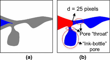
Illustration of the “PSD by MIP simulation” concept in a porous material (400 × 400 pixel). Solid is shown in white, and pore in blue. a pore space after erosion with connectivity check b pore space after dilation. Large pores (pore size d > 25 pixels) are shown in red, according to the “PSD by MIP simulation”
-
Step 3: To determine mercury-intruded pores, the eroded set is dilated as “Step 2” in Sect. 3.1. It finally leads to the opening of the pore space (Fig. 2b).

A smaller radius r is used for mercury intrusion, corresponding to a higher capillary pressure. Consequently, the cumulative porosity ϕ with respect to the pore size can be determined. For both “continuous PSD” and a “PSD by MIP simulation”, a limitation of PM-based image analysis should be pointed out. As discussed by Hilpert et al. [30], this analysis overestimates the pore size when d is very small. It is believed that the very small pores from the microstructure are mostly in a pendular shape. Two distinct principal curvatures exist on the pendular pore surface, with one positive and the other negative. Therefore, the pore size will be overestimated when only one positive curvature is considered. However, this issue is out of the scope of this study. Thus, only one principal curvature is considered for characterizing and comparing the pore structures.
3.3 Specific surface area
In a 3D voxel-based microstructure, each voxel has 6 faces. The voxel face is considered as pore surface when the face is shared by pore voxel and solid voxel. The specific surface area S (m−1) is calculated by:
where A s is the total surface area of the pores (m2) and V b is the bulk volume of the material (m3).
3.4 Connectivity of pores
As mentioned in Sect. 1, the connectivity of water-filled pores will be calculated in this study. Moreover, the connectivity of eroded pore space from the surfaces in Sect. 3.2 needs to be checked. The connectivity of the water-filled pores or the eroded pore space is checked using a cluster-labelling algorithm [33]. As a criterion, hereinafter, only adjacent voxels sharing a common surface are regarded as connected (Fig. 3).

Configurations of two adjacent voxels in porous materials. Two voxels are considered connected when they share a face
3.5 Tortuosity
Tortuosity, as a pore structure-transport parameter, is a measure of the geometric complexity of a porous medium. It characterizes the convoluted pathways of fluid diffusion and electrical conduction through porous media. In the fluid mechanics of porous media, tortuosity is the ratio of the length of a streamline between two points in pore phase to the straight-line distance between the two points. However, the estimation of tortuosity for a porous material is usually subjective. Distinct types of tortuosity, such as geometric, hydraulic, electrical, and diffusive tortuosity have been studied in the literatures [34]. This part of the study aims to compare the tortuosity of water-filled pores between CT-1d and HYMO-1d. Two different tortuosities are calculated, namely a diffusive tortuosity and a geometrical tortuosity.
3.5.1 Diffusive tortuosity: random walk algorithm
Diffusive tortuosity can be determined by simulating self-diffusion in the material. It is noted that, there is a difference between diffusion and self-diffusion of a material. Diffusion refers to the thermal motion of the particles at temperatures above absolute zero. It explains spontaneous movement of particles from a region of higher concentration to a region of lower concentration. Once there is no concentration gradient, the process of diffusion will cease, and self-diffusion governs the movement of particles. With respect to movement of ions in solution, the self-diffusion coefficient D is time-independent. However, in a confining geometry, the process of self-diffusion becomes time-dependent because of local heterogeneity, and a reduced D is expected due to the restriction from solids.
In a porous material, a random walk algorithm can be used to simulate Brownian motion of molecules and the self-diffusion coefficient [35, 36]. Binary 3D digital microstructures of cement pastes are used as inputs. At τ = 0 (the dimensionless integer time), a point in the pore space is randomly chosen as a starting point, from which the walker migrates on discrete voxels corresponding to the pore space. In each integer time step, the walker executes a random jump to one of the nearest face-connected voxels. The jump is not performed if the walker tries to jump to the voxels corresponding to solids, while the time is still incremented by one step. Mean square displacement (MSD) r(τ)2 is a measure of the deviation over time between the position of a particle and some reference position. After a number of jumps, the mean-square displacement r(τ)2 of the walkers from the starting point can be calculated. The self-diffusion coefficient D(t) in a 3D lattice space is defined based on the following equation (Eq. 1):
The diffusive tortuosity τ diff of the pore structure is the limiting value of the ratio of D 0 in the free space to D(t) in the porous media when time t approaches infinity (Eq. 2).
As time t is required to be large enough for a constant self-diffusion coefficient of porous media, it is possible that the walkers jump out of the volume of interest (VOI), which consists of 200 × 200 × 200 voxels representing a volume of 100 × 100 × 100 μm3. To tackle this problem, a larger volume with a periodic boundary is created. 8 mirror copies of the initial VOI are generated and arranged to form a new VOI with a dimension of 200 × 200 × 200 μm3. The new VOI can be used as an element for an infinitely large material by parallel arrangement in 3 different directions. Therefore, the continuity of the pore structure is ensured for a correct estimation of diffusive tortuosity of the materials.
Considering the stochastic nature of the random walk algorithm, simulation on 10,000 walkers is performed by randomly specifying a starting point for each walker in pore phase of the materials. A 2D schematic of random walk is shown in Fig. 4.

Schematic of a porous material (100 × 100 pixels). This figure shows the random walk from point “A” to point “B”. A stepwise explanation is given. The walker starts from point “A” and reaches point “O” after 2500 steps. After another 2500 steps, the walker reaches point “B. This figure also shows the shortest path finding between point “A ′” to point “B ′”. The algorithm of the shortest path finding is presented in Sect. 3.5.2
3.5.2 Geometrical tortuosity: shortest path finding by A* algorithm
Geometrical tortuosity τ geo (Eq. 3) is defined as the ratio of the length of the shortest path connecting two points in the pore space (L e) with respect to the straight connection L between the two points [37]
In porous media, some obstacles (solids) may exist between two points, making the path from one point to another tortuous. Hart et al. [38] first described the A* algorithm for searching shortest paths between the start node to the goal node in graphs.
To find the shortest path between two points, two sets (FRINGE and CLOSED) are included in A* algorithm (Fig. 5). The FRINGE set contains nodes for examining, it holds potential best path nodes that have not yet been considered, starting with the start node. The CLOSED set starts out empty and contains all nodes that have already been visited. Each node also keeps a pointer to its parent node so that the path can be backtracked from the goal to the start. At node n, A* calculates both the actual distance g(n) from the start and the estimated/heuristic distance h(n) to the goal. An evaluation function (Eq. 5) is used to estimate the total distance f(n) between the start and goal nodes
During implementation, A* algorithm selects the node with the lowest \(f\left( n \right)\) from FRINGE set. Then all valid neighboring nodes are put into the FRINGE list. Here the valid neighboring nodes refer to the ones that are not obstacles or not in CLOSED set. A loop is conducted until the goal is reached. Then the \(f\left( n \right)\) value of the goal is considered the length of the shortest path.

A* algorithm for finding the shortest path between two points (A and B) in a porous material (4 × 4 pixels). The obstacles are shown in grey. Representation of the numbers in the nodes is explained in the node at the top right-hand corner
To calculate the geometrical tortuosity, two points (or voxels) in pore space from two opposing surfaces are selected from each sample (HYMO-1d or CT-1d). For example, the two points are located at the coordinates (x, y, 1) and (x, y, 200). Note that the value of the shortest path L e depends on the locations of the two chosen points. In this study, 6 random pairs of points (start and goal) are selected from each sample to study the influence of water saturation on the geometrical tortuosity of water-filled pores in a cement paste. The average value of the geometrical tortuosity will be presented.
Two voxels in pore space from two opposing surfaces of CT-1d are selected for geometrical tortuosity calculation. A straight line connecting these two voxels is vertical to the surfaces where the two voxels are located. A 2D schematic of the shortest path finding between two points (i.e., A′ and B′) is shown in Fig. 4. The calculation of geometrical tortuosity aims to add more significance to the numerically computed tortuosity of water filled pores in digital microstructures.
4 Results and discussion
4.1 “Continuous PSD” and “PSD by MIP simulation”
The cumulative porosities ϕ for CT-1d and HYMO-1d are presented in Fig. 6, where “continuous PSD” and “PSD by MIP simulation” are included. For each sample, the cumulative porosity from “PSD by MIP simulation” evolves behind the one of “continuous PSD”, as pore size decreases. This phenomenon is due to the well-known influence of “ink bottle” and “throat” pores. For both samples, the “continuous PSD” resembles each other, with the variation in cumulative porosity less than 2% at each pore size. In this respect, HYMO-1d has a similar pore structure as CT-1d. However, clear difference can be seen from “PSD by MIP simulation” between two samples: the cumulative porosity varying by 6.25% at pore size of 2 μm. It indicates that two samples with similar “continuous PSD” may have different responses to mercury intrusion.

Cumulative porosities of CT-1d and HYMO-1d
For a clear illustration, pores in the samples are differentiated based on a specified threshold value (named as a “corresponding pore size” d c). Mercury-intruded pores of the samples are illustrated in Fig. 7, with a d c of 2 µm. The figure shows that only the outer parts of CT-1d are intruded with mercury (Fig. 7a), with the mercury-intruded porosity of 11.2% according to Fig. 6. In contrast, mercury is intruded to the inner parts of HYMO-1d (Fig. 7b), with the mercury-intruded porosity of 17.4%. This is because that there exists a smaller pore “neck” in CT-1d, through which the mercury can access the inner parts of the samples.

Visualization of differentiated pores in CT-1d (MIP simulation). Corresponding pore size d c is 2 μm, with mercury-intruded pores in red, empty pores in blue and the solid phase in white
Apart from the cumulative porosity ϕ, differential porosity ϕ d (μm−1) gives another feature of pore structure (Eq. 6). It provides detailed information of the pore microstructure, to which the pore size d is ascribed.
Differential porosity ϕ d of each sample is plotted against the pore size (Fig. 8). It shows that, “continuous PSD” covers a broader range of pore sizes from 1 to 6 µm, compared to “PSD by MIP simulation” where most pores are with a size d < 4 μm. It infers that MIP simulation assigns larger pores to smaller ones, whereby the volume of large pores in the microstructure is underestimated. The “continuous PSD” serves as a basis for determining the misallocation of large pores in the PSD curve determined by MIP simulation. Similar as in Fig. 6, ϕ d from “continuous PSD” of two samples resembles each other. CT-1d has only a slightly lower ϕ d than HYMO-1d for pore sizes between 2 and 4 µm, and a slightly higher ϕ d for other pore sizes. In contrast, ϕ d from “PSD by MIP simulation” of two samples shows a noticeable divergence from each other. For instance, CT-1d has a higher ϕ d than HYMO-1d for pores with a size d < 2 μm, and a lower ϕ d for pores with a size 2 μm < d < 3 μm.

Differential porosity of CT-1d and HYMO-1d

Water saturation and connectivity of water-filled pores in CT-1d and HYMO-1d. The pores dry out with the pore size is equal or larger than the corresponding pore size d c
4.2 Specific surface area
The specific surface areas S of CT-1d and HYMO-1d are 0.30 and 0.23, respectively. For two microstructures with the same porosity, it is believed that the pore structure is finer if the microstructure has a higher specific surface area [26]. Therefore, CT-1d exhibits a finer pore structure compared to HYMO-1d in terms of the specific surface area.
4.3 Connectivity of water-filled pores
The water saturation (referring to Sect. 3.1) and the connectivity of water phase in unsaturated cement pastes (CT-1d and HYMO-1d) are plotted against d c in Fig. 7. Both samples exhibit similar characteristics in terms of water saturation and connectivity of water phase. For each sample, the connectivity of water phase decreases with d c. Most of the water phase is connected when d c > 2 μm. However, the water phase suddenly becomes discontinuous when the d c drops to 2 µm. Note that, the water saturation evolves smoothly as d c decreases. It indicates that there exists a value of water saturation, which is critical for water phase continuity. For the two samples in this study, the critical water saturation is associated with a d c = 2 μm, under which the water phase loses its continuity. According to Mindess et al. [5], water in capillary pores is significant to the transport properties, e.g., permeability. Under the critical water saturation level, the transport path in the capillary pores is cut off. Transport of matters (e.g., ions) has to be via smaller pores (i.e., pores smaller than 0.5 μm that are not resolved in HYMO-1d and CT-1d).
However, it should be pointed out that the connectivity analysis of water-filled capillary pores is influenced by the digital resolution of the microstructures. The connectivity of the pores will be higher when a higher digital resolution is applied [28]. In practice, the connectivity of water-filled capillary pores should be 100%, since at the scale of nanometers the pores in cement pastes are perpetually connected [39]. The connectivity analysis in this study aims to give more information of the capillary pore structures, when similar digital microstructures are used for studying transport properties.
4.4 Tortuosity of water-filled pores
In an unsaturated material, water saturation and its connectivity are two important factors influencing the diffusivity in water-filled pores, because the free diffusion path is affected by the blockage of the air phase. Random walks of 10,000 walkers in two saturated samples (CT-1d and HYMO-1d) are simulated to compute the diffusive tortuosity. Besides, 3 unsaturated microstructures for each sample are studied, with a corresponding pore size d c = 3 μm, d c = 4 μm, and d c = 5 μm, respectively.
Figure 10 shows the diffusive tortuosity τ diff of the water-filled pores in different microstructures. Water saturation is found to play an important role on the diffusive tortuosity of a material. For both samples, τ diff increases with a decreasing water saturation, in the order of “Saturated” < “d c = 5” < “d c = 4” < “d c = 3”. It is mainly caused by the decreased water saturation of water-filled pores, which is indicated in Fig. 9. In general, CT-1d has a higher value of tortuosity than the one of HYMO-1d, for both saturated and unsaturated samples. Note that the unsaturated samples are dried under the same condition (or in other word, dried with the same d c). This reflects the difference in the microstructure, in the sense that CT-1d has a more complex pore structure than HYMO-1d.

Diffusive tortuosity of CT-1d and HYMO-1d. Hereinafter, CT-1d and HYMO-1d refer to saturated microstructures, while d c = 5, d c = 4 and d c = 3 refer to 3 unsaturated microstructures for each sample, with water in pores with the size equal or larger than 5, 4 and 3 µm dried out
Based on the same microstructures as for diffusive tortuosity, the shortest path between two points from two opposing surfaces are calculated, based on which the geometrical tortuosity τ geo of water-filled pores is determined. From Fig. 11, it can be seen that the evolution of geometrical tortuosity τ geo for both samples follows the same trend as the one for diffusive tortuosity (Fig. 10), even though their absolute values are different. Basically, both diffusive tortuosity and geometrical tortuosity can reflect the morphological change in the water-filled pores. They give insights to further studies on unsaturated cementitious materials, i.e. transport properties.

Geometrical tortuosity between two points in HYMO-1d and CT-1d. The designation of samples is referred to Fig. 10
5 Conclusions
In the scope of capillary pores (pores larger than 0.5 μm), this study characterized and compared the pore structures of two cement pastes (CT-1d and HYMO-1d) based on a pore morphology-based image analysis. Water distribution in unsaturated cement pastes, and the related properties, i.e. connectivity and tortuosity of water filled pores, are studied. The following conclusions can be drawn:
-
With the same capillary porosity, HYMO-1d and CT-1d shows a similar “continuous PSD”, but a distinct “PSD by MIP simulation”. MIP simulations reveal that the critical pore neck of CT-1d through which the mercury is accessible to the inner part of the material is smaller than the critical pore neck of HYMO-1d.
-
The specific surface area, the diffusive tortuosity and the geometrical tortuosity of CT-1d are higher than HYMO-1d, indicating a higher complexity of the pore structure in CT-1d with reference to HYMO-1d.
-
In HYMO-1d and CT-1d, the connectivity of water-filled pores has a high value (>90%) when the capillary water saturation level is higher than 50%. The water-filled capillary pores become discontinuous when water saturation level drops to 20%. Besides, the diffusive/geometrical tortuosity of water-filled pores increases with the decrease of the water saturation level.
It should be noted that both microstructures in this study are subjected to various limitations, including the low digital resolution (0.5 μm/voxel) in CT-1d and the assumption of centrical growth of hydration products in HYMO-1d. Thus, this study does not intend to justify any digital microstructure. Rather, it aims to enable a better understanding of the digital microstructures, and to accentuate that multiple parameters (e.g., porosity, specific pore surface area, pore size distribution, connectivity and tortuosity of the pores) should be taken into account when comparing different pore structures.
References
Li S, Roy DM (1986) Investigation of relations between porosity, pore structure, and C1− diffusion of fly ash and blended cement pastes. Cem Concr Res 16:749–759
Basheer L, Kropp J, Cleland DJ (2001) Assessment of the durability of concrete from its permeation properties: a review. Constr Build Mater 15:93–103
Zhang M (2013) Multiscale lattice Boltzmann-finite element modelling of transport properties in cement-based materials. Dissertaiton, Delft University of Technology
Nielsen EP, Geiker MR (2003) Chloride diffusion in partially saturated cementitious material. Cem Concr Res 33:133–138
Mindess S, Young JF, Darwin D (1981) Concrete. Prentice Hall, New York
Cook RA, Hover KC (1999) Mercury porosimetry of hardened cement pastes. Cem Concr Res 29:933–943
Diamond S (2000) Mercury porosimetry: an inappropriate method for the measurement of pore size distributions in cement-based materials. Cem Concr Res 30:1517–1525
Willis KL, Abell AB, Lange DA (1998) Image-based characterization of cement pore structure using wood’s metal intrusion. Cem Concr Res 28:1695–1705
Zhou J, Ye G, Breugel KV (2010) Characterization of pore structure in cement-based materials using pressurization–depressurization cycling mercury intrusion porosimetry (PDC-MIP). Cem Concr Res 40:1120–1128
Breugel KV (1991) Simulation of hydration and formation of structure in hardening cement-based materials. Dissertation, Delft University of Technology
Koenders EAB (1997) Simulation of volume changes in hardening cement-based materials. Dissertation, Delft University of Technology
Bentz DP (2000) CEMHYD3D: a three-dimensional cement hydration and microstructure development modelling package. Version 2.0, National Institute of Standards and Technology Interagency Report 7232
Bishnoi S, Scrivener KL (2009) µic: a new platform for modelling the hydration of cements. Cem Concr Res 39:266–274
Liu L, Sun W, Ye G, Chen H, Qian Z (2012) Estimation of the ionic diffusivity of virtual cement paste by random walk algorithm. Constr Build Mater 28:405–413
Zalzale M (2014) Water dynamics in cement paste: insights from lattice Boltzmann modelling. Dissertation, Swiss Federal Institiute of Technology of Lausanne
Bossa N, Chaurand P, Vicente J, Borschneck D, Levard C, Aguerre-Chariol O, Rose J (2015) Micro- and nano-X-ray computed-tomography: a step forward in the characterization of the pore network of a leached cement paste. Cem Concr Res 67:138–147
Promentilla MAB, Sugiyama T, Hitomi T, Takeda N (2008) Characterizing the 3D pore structure of hardened cement paste with synchrotron microtomography. J Adv Concr Technol 6:273–286
Münch B, Holzer L (2008) Contradicting geometrical concepts in pore size analysis attained with electron microscopy and mercury intrusion. J Am Ceram Soc 91:4059–4067
Garboczi EJ, Bentz DP (1991) Digitised simulation of mercury intrusion porosimetry. Ceram Trans 16:365–380
Ye G (2003) Experimental study and numerical simulation of the development of the microstructure and permeability of cementitious materials. Dissertaiton, Delft University of Technology
Bekri S, Xu K, Yousefian F, Adler PM, Thovert JF, Muller J, Iden K, Psyllos A, Stubos AK, Ioannidis MA (2000) Pore geometry and transport properties in North Sea chalk. J Pet Sci Eng 25:107–134
Do QH, Bishnoi S, Scrivener KL (2013) Numerical simulation of porosity in cements. Transp Porous Media 99:101–117
Bager DH, Sellevold EJ (1975) Mercury porosimetry of hardened cement paste: the influence of particle size. Cem Concr Res 5:171–177
Larson RG, Morrow NR (1981) Effects of sample size on capillary pressures in porous media. Powder Technol 30:123–138
Moro F, Böhni H (2002) Ink-bottle effect in mercury intrusion porosimetry of cement-based materials. J Colloid Interface Sci 246:135–149
Aligizaki KK (2005) Pore structure of cement-based materials: testing, interpretation and requirements. CRC Press, New York
Zhang M, He Y, Ye G, Lange DA, Breugel KV (2012) Computational investigation on mass diffusivity in Portland cement paste based on X-ray computed microtomography (μCT) image. Constr Build Mater 27:472–481
Gallucci E, Scrivener K, Groso A, Stampanoni M, Margaritondo G (2007) 3D experimental investigation of the microstructure of cement pastes using synchrotron X-ray microtomography (μCT). Cem Concr Res 37:360–368
Hazlett R (1995) Simulation of capillary-dominated displacements in microtomographic images of reservoir rocks. Transp Porous Media 20:21–35
Hilpert M, Miller CT (2001) Pore-morphology-based simulation of drainage in totally wetting porous media. Adv Water Resour 24:243–255
Serra J (1982) Image analysis and mathematical morphology, vol 1. Academic Press, London
Bentz DP, Hansen KK, Madsen HD, Vallee F, Griesel EJ (2001) Drying/hydration in cement pastes during curing. Mater Struct 34:557–565
Hoshen J, Kopelman R (1976) Percolation and cluster distribution. I. Cluster multiple labeling technique and critical concentration algorithm. Phys Rev B 14:3438–3445
Ghanbarian B, Hunt AG, Ewing RP, Sahimi M (2013) Tortuosity in porous media: a critical review. Soil Sci Soc Am J 77:1461–1477
Nakashima Y, Kamiya S (2007) Mathematica programs for the analysis of three-dimensional pore connectivity and anisotropic tortuosity of porous rocks using X-ray computed tomography image data. J Nucl Sci Technol 44:1233–1247
Schwartz LM, Banavar JR (1989) Calculation of electrical transport in continuum systems by diffusion simulation. Phys A 157:230–234
Dullien FA (1992) Porous media: fluid transport and pore structure, 2nd edn. Academic, San Diego
Hart PE, Nilsson NJ, Raphael B (1968) A formal basis for the heuristic determination of minimum cost paths. IEEE Trans Syst Sci Cybern 4:100–107
Sant G, Bentz D, Weiss J (2011) Capillary porosity depercolation in cement-based materials: measurement techniques and factors which influence their interpretation. Cem Concr Res 41:854–864
Acknowledgements
Financial support by the Dutch Technology Foundation (STW) for the project 10981-“Durable Repair and Radical Protection of Concrete Structures in View of Sustainable Construction” is gratefully acknowledged.
Funding
This study was funded by the Dutch Technology Foundation (Grant Number 10981).
Author information
Authors and Affiliations
Corresponding author
Ethics declarations
Conflict of interest
The authors declare that they have no conflict of interest.
Rights and permissions
Open Access This article is distributed under the terms of the Creative Commons Attribution 4.0 International License (http://creativecommons.org/licenses/by/4.0/), which permits unrestricted use, distribution, and reproduction in any medium, provided you give appropriate credit to the original author(s) and the source, provide a link to the Creative Commons license, and indicate if changes were made.
About this article

Cite this article
Dong, H., Gao, P. & Ye, G. Characterization and comparison of capillary pore structures of digital cement pastes. Mater Struct 50, 154 (2017). https://doi.org/10.1617/s11527-017-1023-9
Received:
Accepted:
Published:
DOI: https://doi.org/10.1617/s11527-017-1023-9