Generalization enhancement of artificial neural network for turbulence closure by feature selection

Abstract

Feature selection targets for selecting relevant and useful features, and is a vital challenge in turbulence modeling by machine learning methods. In this paper, a new posterior feature selection method based on validation dataset is proposed, which is an efficient and universal method for complex systems including turbulence. Different from the priori feature importance ranking of the filter method and the exhaustive search for feature subset of the wrapper method, the proposed method ranks the features according to the model performance on the validation dataset, and generates the feature subsets in the order of feature importance. Using the features from the proposed method, a black-box model is built by artificial neural network (ANN) to reproduce the behavior of Spalart-Allmaras (S-A) turbulence model for high Reynolds number (Re) airfoil flows in aeronautical engineering. The results show that compared with the model without feature selection, the generalization ability of the model after feature selection is significantly improved. To some extent, it is also demonstrated that although the feature importance can be reflected by the model parameters during the training process, artificial feature selection is still very necessary.

1 Notation

Angle of attack	α	Speed of sound	a ∞
Chord length of airfoil	c	Freestream speed	u ∞
Mach number	Ma = u∞/a∞	Friction velocity	${u}_{\tau }=\sqrt{\tau_w/\rho }$
Reynolds number	Re = u∞c/υ	Drag coefficient	C d
Distance to the wall	d	Vorticity	w
Damping-length constant	A +	Entropy (redefined)	S '  = (p/ργ − 1), (γ = 1.4)
Shear stress at the wall	τ w	Kinetic eddy viscosity	υ t
Wall friction length unit	δυ = υ/uτ	Kinetic viscosity	υ
Boundary layer thickness	δ	Skin friction coefficient	Cf = 2τw/ρ∞u∞2
von Kármán constant	κ	Pressure coefficient	Cp = 2(p − pw)/ρ∞u∞2

2 1 Introduction

In recent years, there has been a surge in research on the combination of machine learning and turbulence. These researches can be divided into two categories according to the model form: classifiers for identifying uncertainty regions and regression models for calculating turbulence-related variables. For the classifier, researchers can use machine learning to recognize the uncertain regions calculated by the Reynolds-Averaged Navier-Stokes (RANS) turbulence model based on experimental or high-fidelity data [1, 2]. The uncertainty of turbulence calculation comes from the ensemble averaging operation of Navier-Stokes (N-S) equation, the functional form of a model, the representation of Reynolds stress and the empirical parameters of the model [3]. Then, a classifier can be constructed to predict the uncertain regions in different flow cases and a better method with higher accuracy can be used to improve the accuracy for these uncertain regions. For the regression, machine learning is mainly used to improve or substitute the conventional RANS model and the subgrid model in large eddy simulation (LES). The linear eddy viscosity models are based on the Boussinesq assumption, which have high efficiency and good robustness, but are eclipsed by anisotropic turbulence, such as large separation and secondary flows. Thus, researchers used machine learning to decrease the discrepancies between RANS results and high-fidelity or experimental data. There are mainly two corresponding solutions. One is to change the governing equation form of the RANS model, such as introducing the correction coefficient or adding the source term to the transport equation [4,5,6,7]. The other is to construct the deviation function by machine learning and then superimpose the results of RANS model and the output of proposed model as the Reynolds stress [8, 9]. Different from the above studies, some studies directly construct the surrogate models of some turbulence variables [10,11,12]. Overall, the achievement is encouraging. In the future, machine learning may play a key role in turbulent modeling of complex flows [13]. With the research deeper and deeper, there are still many problems to be solved, such as feature selection (FS) and insufficient generalization ability, etc. [14, 15]

The feature means each component of the input vector and describes the sample property, which is similar to the independent variable of the function. Thus, the feature plays an important role in the model performance. It is difficult to characterize the data space thoroughly and comprehensively by inadequate features, which leads to low accuracy. On the contrary, redundant features may result in over-fitting of the model and reduce its generalization ability. Generalization generally refers to the performance of a model on unseen datasets. Feature selection is to select relevant and useful features to reduce the computation cost and improve the model performance [16]. For complex problems with unclear mechanism, it is challenging for researchers to extract features straightforwardly. A common way is selecting some related features empirically according to physical knowledge and the specific problem. The result of this way might be accidental. Therefore, an efficient and reliable feature selection algorithm is needed by researchers.

In data-driven turbulence modeling, feature construction and selection are large obstacles for researchers. Many researchers select features according to existing governing equations and theorems or their own physical views. A common recommendation is that the features should be invariant. Invariance property means that values do not change with the translation, reflection and rotation of the coordinate system. Ling et al. [17] compared two methods of integrating invariant property into machine learning models and found that embedding the invariance into the features is more efficient and the corresponding model has better performance. Based on the conclusion, they took five tensor invariants as features and constructed the tensor basis neural network for scalar coefficients of the nonlinear eddy viscosity model. Besides the integrity basis derived by Pope [18], Wu et al. [19] introduced the gradient of turbulent kinetic energy and pressure to consider the effect of strong pressure changes and nonequilibrium. Yin et al. [20] further summarized feature selection criteria based on tensor analysis and flow structure identification. Although some researchers emphasize the invariance property, it is not clear whether the features without this property will definitely reduce the model performance. Wang et al. [21] studied the closure of the subgrid stress in LES and the adopted features are the filtered velocity and first and second order derivatives. Since the geometry and coordinate system of test cases are the same as those of training cases, Cruz et al. [22] took each component of the tensors and vectors as the input feature. Singh et al. [6] adopted the features mainly based on the governing equation of Spalart-Allmaras (S-A) model. The features used in most of the current work are based on physics and belong to the result of feature construction rather than feature selection to a large extent.

There are some common feature selection methods, like filter method, wrapper method and embedded method or some derivation methods based on these three methods [16]. Filter methods rank the features according to the correlation between features and output, which is efficient and priori. One of the common ways to measure the correlation is the Pearson correlation coefficient. Other correlation measurement can be found in the review of Saúl et al. [23] The wrapper methods evaluate the feature subset according to the prediction performance. The exhaustive search of this method becomes an NP-hard problem since there are 2^N feature subsets, where N is the candidate feature number. The embedded methods insert the feature selection into the learning process. The difference of embedded method from the previous two methods is that the learning process and the feature selection process cannot be separated, thus the feature subset applicable to a specific model architecture might not be applicable to other model architectures. In recent years, some hybrid methods of these three methods have been proposed [24, 25]. More information about the feature selection method can be found in many studies [26,27,28,29]. In data-driven turbulence modeling, feature selection methods stated above are not widely used yet.

The principle target of this work is to enhance the model generalization ability through the proposed feature selection algorithm. For high Reynolds number airfoil flows in aerospace, the constructed model in this paper is essentially a black-box model without solving the transport equation, aiming to reproduce the behavior of RANS model. Driven by the data from only one flow case, the constructed model is expected to be effective for various cases with different freestream conditions and airfoils. The rest of this paper is summarized as follows. The second section introduces the methods used in this work, including workflow, modeling strategy, artificial neural network and the feature selection algorithm. The training process is illustrated in the third section, including the datasets and the training method. The fourth section is the results and discussions, which are addressed from the aspects of accuracy and convergence. Conclusions and outlook lie in the fifth section.

3 2 Method

3.1 2.1 Workflow

The workflow includes two parts: neural network training and coupling of the N-S equation solver with the constructed model. The first part aims to obtain a neural network model, of which the performance should be satisfying and convergent. The word “convergent” means that the loss function is hard to be lower. This part mainly consists of three aspects: data acquisition, data preprocessing and model training. Model performance is improved mainly by adjusting model parameters and hyperparameters during the training process. If the performance is not adequate, the input features and training samples can be further optimized in data preprocessing. The target of the second part is to substitute the conventional RANS model with the constructed surrogate model and obtain the results that agree well with those calculated by S-A model. The surrogate model acts as a turbulence solver, as shown in the dot box below. The entire process is shown in Fig. 1, and some details will be addressed later.

Fig. 1

Flow chart for building the turbulence surrogate model

3.2 2.2 Modeling strategy

According to the dimensional analysis, the kinetic eddy viscosity can be expressed as the product of mixing velocity u_mix and mixing length l_mix.

$$ {\upsilon}_t={u}_{mix}{l}_{mix} $$

(1)

The “mixing length” derives from the molecular mean free path in gas dynamics, which was proposed by Prandtl [30]. The algebraic model with zero equation can express turbulent eddy viscosity explicitly in the form of Eq. (1). Generally, two length scales are used to characterize the turbulence from wall to the outer edge of the boundary layer, namely the wall friction scale δ_υ and the boundary layer thickness δ. The δ_υ and δ are corresponding to the inner and outer layers, respectively, where the boundary is around the outer edge of the logarithmic layer. The mixing length of the inner layer is related to the distance to the wall. There are many researches on the scale analysis of the inner layer, and the universality is good in many cases. However, the outer flow variables are only slightly influenced by the wall, and are more disorderly and irregular [31]. Therefore, the scale analysis of the outer layer is more challenging and of less universality. More information about the mixing length is detailed in Granville’s work [32]. The mixing length adopted in this paper is based on the Prandtl-van Driest formulation [33] and limited by the boundary layer thickness of flat plane,

$$ {l}_{mix}=\min \left(\kappa d\left(1-{e}^{-\frac{\mathrm{d}}{d_{y^{+}\approx 1}{A}^{+}}}\right),0.4{\delta}_{flat}\right) $$

(2)

where A⁺ = 26 and κ = 0.4 in this work, ${\mathrm{d}}_{y^{+}\approx 1}$ denotes the estimated wall friction scale, calculated by the function at the following address: https://www.cfd-online.com/Tools/yplus.php. Because it is found that the real wall friction scale leads to worse convergence during the iteration process. Referring to Clauser’s constant eddy viscosity hypothesis [34], the mixing length of the outer layer is the same order with the boundary layer thickness. For convenience, the boundary layer thickness here is approximate to that of the flat plane, since the curvature of the airfoil is small. It should be noted that Eq. (2) is effective qualitatively rather than quantitatively, which is a compromise to the lack of robustness of the constructed neural network model. Once the mixing length is determined, the mixing velocity can be deduced according to Eq. (1). The constructed model in this paper is a nonlinear mapping between mean flow variables and the mixing velocity. Since the modeling strategy includes the distance to the wall, which can be less effective in separated flows, the flow cases in this work are all attached flows.

3.3 2.3 Artificial neural network

The term “neural network” comes from neurology and is often referred to as “artificial neural network” in machine learning. Neuron is the basic unit of a neural network. The number of neurons in each layer is called width and the number of layers is called depth, which are two hyperparameters of a neural network. For a fully-connected neural network, only the neurons in adjacent layers are connected to each other, and the output of the neurons in the previous layer is the input of the neurons in the current layer. The neural network used in this work is shown in Fig. 2.

Fig. 2

Schematic of the fully-connected neural network

The first layer is the input layer while the last layer is the output layer, and the rest is the hidden layers. The parameters of the neuron are called weight and bias. Each neuron contains two operations. The first one is the linear addition between the product of input vector X and weight vector W and bias b,

$$ z=\mathbf{WX}+b $$

(3)

and the second one is the nonlinear activation operation.

$$ y=f(z) $$

(4)

The common activation functions f(·) are Tanh, Sigmoid, Relu, LeakRelu and so on. In this work, Tanh is adopted, see Fig. 3. Since the grid search method is time-consuming, the structure is determined by a trial-and-error approach. Firstly, we fixed the width and tested the effect of depth on the model performance. Then, we fixed the optimal depth and tested the effect of width on the model performance. It was found that the structure (20, 20, 20, 20, 20, 1) is enough for reaching the optimal solution. More neurons do not significantly improve model performances but increase computation time.

Fig. 3

The Tanh activation function

The error back propagation (BP) algorithm based on gradient descent is used to train the neural network. The gradient is calculated by the chain rule to update the parameter values of the neurons. Because the gradient descent algorithm is prone to stop at the local minimum, the global optimum is generally approximated by several training with different initial values. More information about neural networks can be found in many works [35,36,37].

According to the universal approximation theory, neural networks with enough neurons can approximate any measurable functions [38]. The complexity of the neural network can be adjusted by changing the depth and width. The strength of mapping complex nonlinear functions makes neural networks popular with researchers. It has already been used in turbulence computation [10, 39].

3.4 2.4 Feature selection

We do not intend to delve into feature construction that depends on specific problems or researchers’ physical view, but rather try to select some features that are helpful to model performance from existing candidate features. Although we assume that the neural network itself can play a role in feature selection more or less in the training process, the important role played by artificial feature selection is irreplaceable according to our own experience.

The proposed feature selection method includes two parts. The first one is measuring the numerical space of the features and kicking off those with obvious extrapolation according to the mean extrapolation distance (MED). The second one is ranking the feature and determining the feature subset according to the model performance. The whole process is shown in Fig. 4 and to be more specifically, it includes the following steps.

• Step 1: Get the dataset $\mathtt{D}=\left\{\left({\mathbf{Q}}_{\mathtt{D}},{\mathbf{y}}_{\mathtt{D}}\right),{\mathbf{Q}}_{\mathtt{D}}\in {\mathrm{\mathbb{R}}}^{l_{\mathtt{D}}\times m},{\mathbf{y}}_{\mathbf{D}}\in {\mathrm{\mathbb{R}}}^{l_{\mathtt{D}}\times 1}\right\}$ and $\mathtt{T}=\left\{\left({\mathbf{Q}}_{\mathtt{T}},{\mathbf{y}}_{\mathtt{T}}\right),{\mathbf{Q}}_{\mathtt{T}}\in {\mathrm{\mathbb{R}}}^{l_{\mathtt{T}}\times m},{\mathbf{y}}_{\mathtt{T}}\in {\mathrm{\mathbb{R}}}^{l_{\mathtt{T}}\times 1}\right\}$, where Q denotes the feature vectors, y the labels, m the number of features, ${l}_{\mathtt{D}}$ and ${l}_{\mathtt{T}}$ the sample number of $\mathtt{D}$ and $\mathtt{T}$, respectively. Normalize each feature and the output of $\mathtt{D}$ to [−1, 1], and normalize the dataset $\mathtt{T}$ according to the corresponding minimum and maximum values from $\mathtt{D}$. Mark the space domain and the domain boundary formed by each feature and the output of $\mathtt{D}$ as Ω_i and ∂Ω_i, respectively, where i = 1, 2…, m. Put the sample of $\mathtt{T}$ in corresponding domain according to the feature and regard those samples outside the domain boundary as extrapolation samples. Calculate the MED of each feature by Eq. (5) and remove the features with large MED values. Denote the number of the remaining features as n. Extract the remaining features and the output from $\mathtt{D}$ and $\mathtt{T}$, and reshape the datasets as $\overline{\mathtt{D}}=\left\{\left({\mathbf{Q}}_{\overline{\mathtt{D}}},{\mathbf{y}}_{\mathtt{D}}\right),{\mathbf{Q}}_{\overline{\mathtt{D}}}\in {\mathrm{\mathbb{R}}}^{l_{\mathtt{D}}\times n},{\mathbf{y}}_{\mathbf{D}}\in {\mathrm{\mathbb{R}}}^{l_{\mathtt{D}}\times 1}\right\}$ and $\overline{\mathtt{T}}=\left\{\left({\mathbf{Q}}_{\overline{\mathtt{T}}},{\mathbf{y}}_{\mathtt{T}}\right),{\mathbf{Q}}_{\mathtt{T}}\in {\mathrm{\mathbb{R}}}^{l_{\mathtt{T}}\times n},{\mathbf{y}}_{\mathtt{T}}\in {\mathrm{\mathbb{R}}}^{l_{\mathtt{T}}\times 1}\right\}$, respectively.

  Fig. 4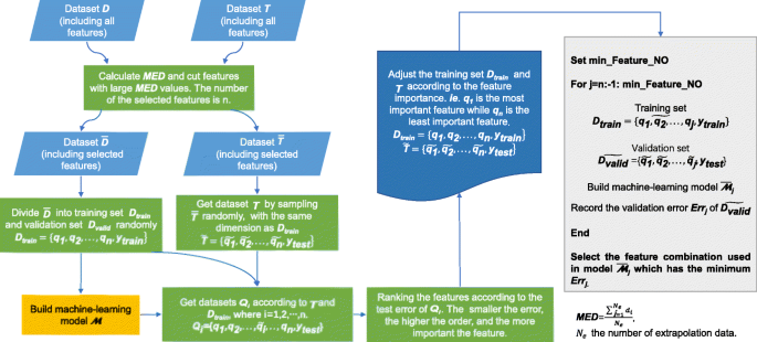

  

  The procedure of feature selection

$$ \mathrm{MED}=\frac{\sum \limits_{i=1}^{N_e}{d}_i}{N_e} $$

(5)

where N_e is the number of the extrapolation samples.

• Step 2: Divide the dataset $\overline{\mathtt{D}}$ into training set ${\mathtt{D}}_{\mathtt{train}}$ and validation set ${\mathtt{D}}_{\mathtt{valid}}$ randomly, where ${\mathtt{D}}_{\mathtt{train}}=\left\{\left({\mathbf{q}}_{\mathbf{1}},{\mathbf{q}}_{\mathbf{2}},\dots, {\mathbf{q}}_{\mathbf{n}},{\mathbf{y}}_{\mathbf{train}}\right),{\mathbf{q}}_i\in {\mathrm{\mathbb{R}}}^{l_{\mathtt{train}}\times 1},{\mathbf{y}}_{\mathbf{train}}\in {\mathrm{\mathbb{R}}}^{l_{\mathtt{train}}\times 1},i=1,2,\dots, n\right\}$. Construct a neural network M according to ${\mathtt{D}}_{\mathtt{train}}$ and ${\mathtt{D}}_{\mathtt{valid}}$. Create a new dataset $\overset{\sim }{\mathtt{T}}=\left\{\left(\overset{\sim }{{\mathbf{q}}_{\mathbf{1}}},\overset{\sim }{{\mathbf{q}}_{\mathbf{2}}},\dots, \overset{\sim }{{\mathbf{q}}_{\mathbf{n}}},{\mathbf{y}}_{\mathtt{test}}\right),\overset{\sim }{{\mathbf{q}}_i}\in {\mathrm{\mathbb{R}}}^{l_{\mathtt{train}}\times 1},{\mathbf{y}}_{\mathtt{test}}\in {\mathrm{\mathbb{R}}}^{l_{\mathtt{train}}\times 1},i=1,2,\dots, n\right\}$ by selecting ${l}_{\mathtt{train}}$ samples from $\overline{\mathtt{T}}$. Replace the feature of ${\mathtt{D}}_{\mathtt{train}}$ by the same feature of $\overset{\sim }{\mathtt{T}}$ one by one and combine the output of $\overset{\sim }{\mathtt{T}}$, thus, we can get n datasets ${\mathtt{Q}}_{\mathtt{i}}$, where i = 1, 2…, n.

$$ {\mathtt{Q}}_{\mathtt{i}}=\Big\{\left({\mathbf{q}}_{\mathbf{1}},{\mathbf{q}}_{\mathbf{2}},\dots, \overset{\sim }{{\mathbf{q}}_{\mathtt{i}}},\dots, {\mathbf{q}}_{\mathbf{n}},{\mathbf{y}}_{\mathtt{test}}\right) $$

Test the model by datasets ${\mathtt{Q}}_{\mathtt{i}}$ and get the test errors. Rank the features according to the test errors. The smaller the error, the more important the feature and the higher the rank.

• Step 3: Adjust the features of ${\mathtt{D}}_{\mathtt{train}}$ and $\overset{\sim }{\mathtt{T}}$ according to the feature importance and shape them as the following form:

$$ {\displaystyle \begin{array}{l}\kern1.25em \mathrm{Feature}\ \mathrm{Importance}:1,\kern0.75em 2,\dots, \kern1.5em n\\ {}\kern2.75em {\mathtt{D}}_{\mathtt{train}}=\left\{{\mathbf{q}}_{\mathbf{1}},{\mathbf{q}}_{\mathbf{2}},\dots, {\mathbf{q}}_{\mathbf{n}},{\mathbf{y}}_{\mathbf{train}}\right\}\\ {}\kern2.75em \overset{\sim }{\mathtt{T}}=\left\{\overset{\sim }{{\mathbf{q}}_{\mathbf{1}}},\overset{\sim }{{\mathbf{q}}_{\mathbf{2}}},\dots, \overset{\sim }{{\mathbf{q}}_{\mathbf{n}}},{\mathbf{y}}_{\mathtt{test}}\right\}\end{array}} $$

Create the training set $\overset{\sim }{{\mathtt{D}}_{\mathtt{train}}}$ and validation set $\overset{\sim }{{\mathtt{D}}_{\mathtt{valid}}}$ by selecting the first j features from ${\mathtt{D}}_{\mathtt{train}}$ and $\overset{\sim }{\mathtt{T}}$, respectively. Then, construct a neural network according to $\overset{\sim }{{\mathtt{D}}_{\mathtt{train}}}$ and $\overset{\sim }{{\mathtt{D}}_{\mathtt{valid}}}$, and record the validation error Err_j on $\overset{\sim }{{\mathtt{D}}_{\mathtt{valid}}}$. The feature number j increases from min _ Feature _ NO set by the user to n one by one. Finally, select the feature subset with the minimal validation error.

In this paper, datasets $\mathtt{D}$ and $\mathtt{T}$ are composed of 2525 and 5437 samples, respectively. These samples are obtained from different flow cases (see Table 1) using the sample selection algorithm described below. The flow cases are sampled through the Latin hypercube sampling method (LHS), and the sampling space is Ma ∈ [0.1, 0.5], Re ∈ [2 × 10⁶, 8 × 10⁶], α ∈ [0°, 5°]. The total candidate features before feature selection are shown in Table 2, where p denotes the pressure, x and y denote the streamline and normal direction of the freestream respectively and the subscripts denote the partial derivative in the direction. The sign function sgn() is defined as follows.

$$ \operatorname{sgn}(x)=\left\{\begin{array}{l}-1\kern0.5em x<0\\ {}0\kern0.75em x=0\\ {}\begin{array}{cc}1&\ x>0\end{array}\end{array}\right. $$

(6)

Table 1 The flow cases of dataset $\mathtt{D}$ and $\mathtt{T}$ used for feature selection

Table 2 The total candidate features

It can be found that the candidate features are not limited to those with invariant property. Some features have invariant property, such as ${u}_i\frac{\partial p}{\partial {x}_i}$ and S ' /Ma², while others don’t, such as velocity vector and its derivatives, which are invariant to translation but not to rotation. According to step 1, the MED of each feature can be calculated (see Fig. 5) and the space domain formed by each feature and the output of dataset $\mathtt{D}$ and $\mathtt{T}$ can also be plotted. For example, the space domain of some features can be seen in Fig. 6. After removing the features with large MED, the remaining features are (q₅, q₈, q₁₀, q₁₁, q₁₂, q₁₃, q₁₄). For step 2, the mean square error (MSE) of 7 datasets ${\mathtt{Q}}_1-{\mathtt{Q}}_7$ is shown in Fig. 7. Thus, the feature importance is q₈ > q₁₃ > q₅ > q₁₂ > q₁₄ > q₁₀ > q₁₁ according to the MSE. In step 3, the min _ Feature _ NO is set to be 3, which means that the features q₈, q₁₃, q₅ are necessary.

Fig. 5

The MED of each feature

Fig. 6

The numerical distribution of some features of dataset $\mathtt{D}$ and $\mathtt{T}$

Fig. 7

The model performance on dataset ${\mathtt{Q}}_1-{\mathtt{Q}}_7$

Starting from these three features, an individual feature subset can be generated as the feature number increases by one in the order of the feature importance and a corresponding neural network model can be constructed. The best feature subset can be found by the model performance on validation set. In order to avoid the influence of occasionality, the model is trained three times for each feature subset, and the model performance is measured according to the mean value of the errors on validation set. As is shown in Fig. 8 where the horizontal axis means the feature number of the feature subset, the model performance is the best when the first four features are adopted. Therefore, the features used to construct the model hereinafter are (q₈, q₁₃, q₅, q₁₂).

Fig. 8

The model performance based on different feature subsets

4 3 Model training

4.1 3.1 Dataset

The source data used in this paper is computed by the CFD solver coupled with the S-A model [40], where the transport equation of the S-A model is as follows.

$$ {\mu}_T=\rho \hat{\upsilon}{f}_{v1} $$

(7)

$$ \frac{D\hat{\upsilon}}{D\mathrm{t}}={C}_{b1}\left(1-{f}_{t2}\right)\hat{S}\hat{\upsilon }+\frac{1}{\sigma}\left\{\nabla \cdot \left[\left(\upsilon +\hat{\upsilon}\right)\nabla \hat{\upsilon}\right]+{C}_{b2}{\left(\nabla \hat{\upsilon}\right)}^2\right\}-\left({C}_{w1}{f}_w-\frac{C_{b1}}{\kappa^2}{f}_{t2}\right){\left(\frac{\hat{\upsilon}}{d}\right)}^2 $$

(8)

The governing equations are solved by the pseudo-time-marching method. The cell-centered finite volume method is used and the spatial discretization is the AUSM+UP scheme with second-order accuracy. The governing equations are nondimensionalized by the mean aerodynamic chord c, speed of sound a_∞ and freestream density ρ_∞. The airfoil surface is set to be wall with no-slip condition and the far field is pressure-far-field without reflection. When the variation of drag coefficient between 1000 iterations is less than 1 × 10⁻⁵, the flow field is set to be converged. Hybrid meshes are used. The grid near the wall is quadrilateral with a growth rate of 1.2 and the outer grid is triangular. The height of the first layer at the wall satisfies y⁺ < 1. The benchmarks of NACA0012 and RAE2822 airfoils are adopted to validate the code and the corresponding freestream condition is shown in Table 3. The result of the CFL3D and experiment can be referred to [41,42,43]. Both of the agreement of C_p and C_f are good, see Figs. 9 and 10.

Table 3 The freestream condition of the benchmark cases

Fig. 9

The comparison of surface pressure C_p and skin friction coefficient C_f of NACA0012 airfoil

Fig. 10

The comparison of surface pressure C_p and skin friction coefficient C_f of RAE2822 airfoil

In this paper, there is only one training case, and its freestream condition is Ma = 0.27, AOA = 2.45°, Re  = 3 × 10⁶. Two thousand five hundred and twenty-five data pairs were generated by the sample selection algorithm, and 1/5 of them were selected randomly as the validation dataset, while the rest were used as the training dataset. A total of 68 flow cases were used as the test cases, 60 of which are shown in Fig. 11 and the rest cases will be illustrated later. The reason for this design of test cases is that we attempt to find whose change of the freestream condition (Ma, Re, AOA) is more challenging for the model performance, which might be helpful for future work.

Fig. 11

Training (blue square) and test (orange circle) cases. a Re = 3 × 10⁶. b Ma = 0.27

4.2 3.2 Data process

4.2.1 3.2.1 Sample selection

The goal of sample selection, in our opinion, is to select as few samples as possible to represent as much of the original sample space as possible. In other words, the diversity of physical behaviors contained in the original sample space should be retained as much as possible. The sample selection method used in this work is a combination of the law of the wall and recursive algorithm. The whole process can be achieved by two steps:

• Step 1: Divide the flow field into several subzones according to lny⁺, and the size of each subzone is a set value Δx.

• Step 2: Set the standard correlation value cc _ std. Take the first data in the subzone as the first sample. For each subzone, starting loop from the second data, calculate the correlation coefficient cc between each data and all samples of the current subzone, and denote the maximal cc as cc _ maximum. If cc _ maximum < cc _ std, then the corresponding data is a new sample; otherwise, the data is redundant and should be removed. Loop the current step for all subzones.

The formula of correlation coefficient is,

$$ cc=\frac{{\mathbf{g}}_1\cdot {\mathbf{g}}_2}{\left\Vert {\mathbf{g}}_1\right\Vert \left\Vert {\mathbf{g}}_2\right\Vert } $$

(9)

where g denotes the vector composed by the input features and output. The specific algorithm is shown in Table 4.

Table 4 The sample selection algorithm

It should be noted that before the sample selection and during the coupling process later, the data of cells whose Reynolds stress is near zero in the far field is eliminated according to the redefined entropy S'  < 2 × 10⁻⁵. In this work, we applied the sample selection to the training case. And we set Δx = 0.2 and cc _ std = 0.999737. The number of subzone is 59. The data number before and after sample selection is 8328 and 2525, respectively. The comparison of data distribution before and after sample selection is shown in Fig. 12 when this method is applied to the training case. It can be found from the figure that, among the selected samples, many of them lie in the leading edge and trailing edge where the flow field changes rapidly. And the data at middle airfoil is obviously sparse, while there is only a few data in the far field and wake region.

Fig. 12

Distribution of the total data and selected data for the training case Ma = 0.27, AOA = 2.45°, Re  = 3 × 10⁶. a Inner layer. b Outer layer

4.2.2 3.2.2 Postprocess

For the samples at the edge of model performance, the model outputs are probably outliers, resulting in negative eddy viscosity. In this case, eddy viscosity is forced to be non-negative. In addition, there may also be the phenomenon of “burr”, that is the small jump of the outputs among adjacent cells. In order to obtain a smooth flow field, spatial smoothing is introduced to smooth the eddy viscosity field calculated by the model at each iteration.

$$ {\mu}_t=\frac{\mu_t+\beta \sum \limits_i^N{\mu_t}^i}{1+\beta N} $$

(10)

where i denotes the i_th neighboring cell, N the total number of neighboring cells. β is the weight of neighboring cells, thus, the larger the β, the better the smoothness. But the eddy viscosity in the boundary layer changes sharply and non-linearly along the normal direction of the wall. Since Eq. (10) is linear, the error can be evitable. And the larger the β, the larger the error. It is a trade-off between smoothness and accuracy. We recommend small values for test cases which are similar to the training case and large values for test cases which deviate a lot from the training case. In this work, we set β ∈ [0.2, 1]. All the flow cases involved in this paper are steady. Therefore, the final turbulent field should be convergent. During the iteration process, we found that the turbulence field calculated by the model is convergent on the whole, but there are slight oscillations of the eddy viscosity of some cells from time to time. The slight oscillation in turn causes the residual oscillation of the N-S solver. In order to restrain such unreasonable oscillation, when the residual value of N-S solver is less than 1 × 10^‐5, the mean variation of eddy viscosity ∑Δμ_t/M between adjacent iteration steps is limited to be monotonically non-increasing, where M is the number of the total cells. More specifically, denote the value of ∑Δμ_t/M at current step k as ∑Δμ_t^k/M, where Δμ_t = |μ_t^k − μ_t^k − 1|. At each iteration step, set ∑Δμ_t/M = min(∑Δμ_t/M, ∑Δμ_t^k/M) and cycle the whole grid cells. If the variation of eddy viscosity between current and forward steps satisfies Δμ_t >  ∑ Δμ_t/M, then set μ_t^k = μ_t^k − 1 + sgn(μ_t^k − μ_t^k − 1) ×  ∑ Δμ_t/M. It is found that the influence of this limitation on the final results can be ignored.

4.3 3.3 Training process

If the loss function is simply defined as mean square error, then the relative error of the model will be large for samples with small output value. As far as this work is concerned, the above trouble happens in the near wall region, and thus the model is prone to perform poorly. Furthermore, the high shear strain rate here will lead to unreasonable results of Reynolds stress and skin friction distribution. Therefore, in the training process, the accuracy of Reynolds shear stress is considered as a constraint for the region y⁺ < 30. In other words, the accuracy of the samples in near wall region is improved through increasing the weight in the loss function by the constraint term.

The constructed model needs to be coupled with the N-S solver like conventional turbulence models. Therefore, the robustness of the model should be enhanced during the training process to avoid the high sensitivity of output to the slight change of input. Two tricks are used. One is that we included the L1-norm and L2-norm regulation in the loss function. The other is that we introduced the stability training (ST) after the normal training process. The principle of stability training is to enhance the model robustness through adding some random noise to the original samples. The random noise used in this work is uniformly distributed with a magnitude less than ±5% of the original sample.

$$ \overset{\sim }{\boldsymbol{X}}=\left(1\pm 5\%\right)\boldsymbol{X} $$

(11)

where $\overset{\sim }{\boldsymbol{X}}$ is called random perturbation copy. The model output of $\overset{\sim }{\boldsymbol{X}}$ is denoted as $\overset{\sim }{\boldsymbol{Y}}$. The stability loss term is defined as,

$$ {L}_{stability}=\sqrt{\sum \limits_i^M{\left({\boldsymbol{Y}}_i-{\overset{\sim }{\boldsymbol{Y}}}_i\right)}^2} $$

(12)

The loss function of ST is:

$$ Loss= MSE+\underset{Regulation\ loss}{\underbrace{\lambda_1{\left\Vert \mathbf{w}\right\Vert}_1+{\lambda}_2{\left\Vert \mathbf{w}\right\Vert}_2}}+\underset{Constraint\ loss}{\underbrace{\lambda_3\left({\left\Vert {\tau_{SA}}^{uv}-{\tau_{ML}}^{uv}\right\Vert}_2\right)}}+\underset{Stability\ loss}{\underbrace{\lambda_4{L}_{stability}}} $$

(13)

where

$$ MSE=\frac{\sum \limits_i^N{\left({y}_i-{f}_i\right)}^2}{N},\kern1.75em {y}_i:\mathrm{label},\kern0.5em {f}_i:\mathrm{model}\ \mathrm{output} $$

(14)

More details on stability training can be referred to the work of Zheng et al. [44] The model training is implemented on PyTorch [45], and the related parameters are shown in Table 5. There are five components in the loss function and the magnitude of each one can be different during the training process. If the magnitude of one component is much larger than that of the others, then the effect of the other components will be suppressed. Thus, the multiplier λ₁ − λ₄ is introduced to make the magnitude of each component on the same order. It should be noted that the error function of the validation set does not include the stability loss term during normal training, which is defined as:

$$ Error= MSE+{\lambda}_3\left({\left\Vert {\tau}_{SA}-{\tau}_{ML}\right\Vert}_2\right) $$

(15)

During the stability training, the error function is redefined as:

$$ {Error}^{ST}= MSE+{\lambda}_3\left({\left\Vert {\tau}_{SA}-{\tau}_{ML}\right\Vert}_2\right)+{\lambda}_4{L}_{stability} $$

(16)

The training process is over when the error function no longer drops within 500 steps.

Table 5 The training parameters

5 4. Results and discussions

Since C_d and C_f are sensitive to the eddy viscosity field, this section mainly assesses the accuracy of the constructed model from these two aspects. The model performance is expected to be good in the test space Ma ∈ [0.1, 0.5], Re ∈ [2 × 10⁶, 10 × 10⁶], α ∈ [0°, 5°]. First of all, we calculate the relative error of C_d for all the test cases in Fig. 11. The error contour of the test space can be obtained by interpolation of the scattered cases, as shown in Fig. 13. It can be found that the relative error varies regularly with the angle of attack and Ma number for cases with fixed Re number. The relative error is smaller with the increase of angle of attack and larger with the increase of Ma number. However, the variation of the relative error is ambiguous with angle of attack and Re number for cases with fixed Ma number. On the whole, the relative error increases with the increase of angle of attack and Re number. The above analysis is qualitative and rough. More detailed and quantitative information is shown in Fig. 14. When α < 3°, the influence of angle of attack on model performance is not obvious. When α > 3°, the C_d calculated by the constructed model tends to be small with the increase of angle of attack. In addition, the C_d is smaller than that calculated by the S-A model as the Re number increases.

Fig. 13

The relative error contour of C_d of the test cases

Fig. 14

The relative error of C_d of the test cases, where Rela Dis = (C_{d, ML} − C_{d, SA})/C_{d, SA}

It can be found from the above results that the model performance tends to be poor at some boundaries of the test space, which is helpful to speculate the model performance in the whole test space. The freestream conditions of the eight boundary point cases and the corresponding relative errors of C_d are listed in Table 6. Only case C6 slightly exceeds 5%, while the other cases are all lower than 4%. The corresponding skin friction coefficient distribution is shown in Fig. 15. The cases C7 and C6 correspond to the best and worst model performance, respectively.

Table 6 The relative error of C_d of the eight boundary point cases in the test space

Fig. 15

The C_f comparison of the eight boundary point cases of NACA0012 airfoil

In order to validate the proposed sample selection and feature selection algorithms, two models were constructed respectively under the same model architecture: one is without sample selection and feature selection and the other is only without sample selection. Take the two cases of NACA0012 airfoil as examples, and the comparison of C_f calculated by the three models is shown in Fig. 16. The result is obviously wrong without feature selection, although the accuracy of the lower surface at the leading edge is better for case C6. This indicates that more features do not mean better model performance, and the ability of neural network to select features automatically is limited. Elaborate feature selection is necessary. Sample selection has negligible influence on the result, except for slight deviation at the leading edge of the airfoil, which indicates that the proposed sample selection algorithm is feasible and the selected samples preserve the data space and diversity of the original dataset. Thus, what should be focused on is the diversity rather than the number of samples. In terms of these two cases, the C_f agreement is very good at the upper surface, which is obviously better than that of the lower surface. The deficiency mainly manifests in two aspects. One is around the peak value of C_f at the leading edge, where the flow variables change dramatically. The other lies in the lower surface from the leading edge to the 0.4 times of chord length, where the C_f calculated by the model is smaller. When generalized to the RAE2822 airfoil, the model shows similar performance, as is shown in Fig. 17.

Fig. 16

The C_f comparison of NACA0012 airfoil. a C7. b C6

Fig. 17

The C_f comparison of RAE2822 airfoil. a C7. b C6

When the constructed models can be coupled with N-S solvers like conventional models, the research is of more practical significance. However, the error propagation between the Reynolds stress and the time-averaged flow field is a challenge for most of the research. Wu et al. [47] explained the stability of different closure models according to the local condition number. Cruz et al. [22] suggested using the Reynolds force vector instead of the Reynolds stress tensor as the model output. For the steady cases in this work, we expect that the convergent solution can be obtained when coupling the model with the N-S solver. Although we enhance the model robustness and the smoothness of the eddy viscosity field by stability training and space-time smoothing and the eddy viscosity model has its own stability advantage, these are still not enough to counteract the high sensitivity of time-averaged field to Reynolds stress, which causes the residual oscillation and the slower convergence.

Since the convergence process of all cases is similar, we take the case C6 of NACA0012 airfoil as an example to make further analysis for the sake of convenience. In each iteration step, we tracked the Reynolds shear stress variation between the current step and the previous step of the cell with maximal residual value. In this regard, the change of S-A model decays fast and smoothly, while that of the ML model decays slower and has large oscillations frequently, as is shown in Fig. 18. The oscillations of Reynolds stress variation derive from those of the model output, which disturb the convergence of the mean flow field and lead to the residual oscillations. The location of the cells with maximum residual was documented after 6 × 10⁴ pseudo steps, see Fig. 19(a). Since many symbols overlap each other, we further count the percentage of the symbols in the same location in all symbols, see Fig. 19(b). It can be found that most of the cells with maximum residual are in the buffer layer and near the inner edge of the log layer and the majority lie in the back part of the airfoil.

Fig. 18

The residual evolution for case C6 of NACA0012 airfoil

Fig. 19

The location and percentage of the cells with maximum residual after 6 × 10⁴ pseudo steps for case C6 of NACA0012 airfoil

6 5. Conclusion and outlook

In this paper, a feature selection method is developed to improve the generalization ability of machine learning models in turbulent flows. The method selects the features by three steps: firstly, measure the numerical distribution characteristics of the training and validation datasets according to the mean extrapolation distance and eliminate the features with obvious numerical extrapolation; secondly, construct a model with all features, then test and rank the effect of each feature on the model performance; finally, generate the feature subsets according to the feature importance and evaluate the model performance that each feature subset can achieve, then select the feature subset with optimal model performance. The proposed method avoids the shortcoming of priori of feature importance ranking and low efficiency of exhaustive research.

Using the features from the proposed method, a turbulence surrogate model is constructed with artificial neural networks driven by the flow field data calculated by N-S solver coupled with S-A model. The training data is selected from only one flow case, and 70 flow cases with different freestream conditions and airfoils are tested. The results indicate that the generalization ability of the constructed model is amazing. The model driven by only one flow case performs well in the whole designed test space after the feature selection. The relative error of the drag coefficient is within 5% for almost all the test cases.

This work mainly validates the proposed feature selection method. In future work, it can be compared with some existing feature selection methods for effect and efficiency.

References

Ling J, Templeton J (2015) Evaluation of machine learning algorithms for prediction of regions of high Reynolds averaged Navier stokes uncertainty. Phys Fluids 27(8):042032–042094. https://doi.org/10.1063/1.4927765
Singh AP, Duraisamy K (2016) Using field inversion to quantify functional errors in turbulence closures. Phys Fluids 28(4):045110. https://doi.org/10.1063/1.4947045
Duraisamy K, Iaccarino G, Xiao H (2019) Turbulence modeling in the age of data. Annu Rev Fluid Mech 51(1):357–377. https://doi.org/10.1146/annurev-fluid-010518-040547
Matai R, Durbin PA (2019) Zonal eddy viscosity models based on machine learning. Flow Turbulence Combustion 103(1):93–109. https://doi.org/10.1007/s10494-019-00011-5
Parish EJ, Duraisamy K (2016) A paradigm for data-driven predictive modeling using field inversion and machine learning. J Comput Phys 305:758–774. https://doi.org/10.1016/j.jcp.2015.11.012
Singh AP, Medida S, Duraisamy K (2017) Machine-learning-augmented predictive modeling of turbulent separated flows over airfoils. AIAA J 55(7):2215–2227. https://doi.org/10.2514/1.J055595
Zhang ZJ, Duraisamy K (2015) Machine learning methods for data-driven turbulence modeling. AIAA 2015-2460. 22nd AIAA Computational Fluid Dynamics Conference, Dallas, 22-26 June 2015
Wang JX, Wu JL, Xiao H (2017) A physics informed machine learning approach for reconstructing Reynolds stress modeling discrepancies based on DNS data. Phys Rev Fluids 2(3):034603
Xiao H, Wu JL, Wang JX et al (2017) Physics-informed machine learning for predictive turbulence modeling: Progress and perspectives. AIAA 2017–1712. 55th AIAA Aerospace Sciences Meeting, Grapevine, 9 - 13 January 2017
Ling J, Kurzawski A, Templeton J (2016) Reynolds averaged turbulence modelling using deep neural networks with embedded invariance. J Fluid Mech 807:155–166. https://doi.org/10.1017/jfm.2016.615
Zhu L, Zhang W, Kou J, Liu Y (2019) Machine learning methods for turbulence modeling in subsonic flows around airfoils. Phys Fluids 31(1):015105. https://doi.org/10.1063/1.5061693
Zhu L, Zhang W, Sun X, Liu Y, Yuan X (2021) Turbulence closure for high Reynolds number airfoil flows by deep neural networks. Aerosp Sci Technol 110:106452. https://doi.org/10.1016/j.ast.2020.106452
Nathan KJ (2017) Deep learning in fluid dynamics. J Fluid Mech 814:1–4. https://doi.org/10.1017/jfm.2016.803
Brunton SL, Noack BR, Koumoutsakos P (2019) Machine learning for fluid mechanics. Annu Rev Fluid Mech 52(1):477–508. https://doi.org/10.1146/annurev-fluid-010719-060214
Zhang W, Zhu L, Liu Y et al (2019) Progresses in the application of machine learning in turbulence modeling. Acta Aerodynam Sin 37(3):444–454
Guyon I, Elisseeff A (2006) An introduction to feature extraction. In: Guyon I, Nikravesh M, Gunn S, Zadeh LA (eds) Feature extraction: foundations and applications. Springer:Berlin Heidelberg, Berlin, Heidelberg, pp 1–25. https://doi.org/10.1007/978-3-540-35488-8
Ling J, Jones R, Templeton J (2016) Machine learning strategies for systems with invariance properties. J Comput Phys 318:22–35. https://doi.org/10.1016/j.jcp.2016.05.003
Pope SB (2000) Turbulent flows. Turbulent Flows 12(11):806–2021. https://doi.org/10.1088/0957-0233/12/11/705
Wu JL, Xiao H, Paterson E (2018) Physics-informed machine learning approach for augmenting turbulence models: a comprehensive framework. Phys Rev Fluids 3(7):074602. https://doi.org/10.1103/PhysRevFluids.3.074602
Yin Y, Yang P, Zhang Y et al (2020) Feature selection and processing of turbulence modeling based on an artificial neural network. Phys Fluids 32(10):105117. https://doi.org/10.1063/5.0022561
Wang Z, Luo K, Li D, Tan J, Fan J (2018) Investigations of data-driven closure for subgrid-scale stress in large-eddy simulation. Phys Fluids 30(12):125101. https://doi.org/10.1063/1.5054835
Cruz MA, Thompson RL, Sampaio LE et al (2019) The use of the Reynolds force vector in a physics informed machine learning approach for predictive turbulence modeling. Comput Fluids 192:104258. https://doi.org/10.1016/j.compfluid.2019.104258
Solorio-Fernández S, Carrasco-Ochoa JA, Martínez-Trinidad JF (2020) A review of unsupervised feature selection methods. Artif Intell Rev 53(2):907–948. https://doi.org/10.1007/s10462-019-09682-y
Solorio-Fernández S, Carrasco-Ochoa JA, Martínez-Trinidad JF (2016) A new hybrid filter–wrapper feature selection method for clustering based on ranking. Neurocomputing 214:866–880. https://doi.org/10.1016/j.neucom.2016.07.026
Bermejo P, De La Ossa L, Gámez JA et al (2012) Fast wrapper feature subset selection in high-dimensional datasets by means of filter re-ranking. Knowl-Based Syst 25(1):35–44. https://doi.org/10.1016/j.knosys.2011.01.015
Chandrashekar G, Sahin F (2014) A survey on feature selection methods. Comput Electr Eng 40(1):16–28. https://doi.org/10.1016/j.compeleceng.2013.11.024
Guyon I, Elisseeff A (2003) An introduction to variable and feature selection. J Mach Learn Res 3(Mar):1157–1182
Cai J, Luo J, Wang S, Yang S (2018) Feature selection in machine learning: a new perspective. Neurocomputing 300:70–79. https://doi.org/10.1016/j.neucom.2017.11.077
Yu L, Liu H (2004) Efficient feature selection via analysis of relevance and redundancy. J Mach Learn Res 5(Oct):1205–1224
Erhard DP, Etling D, Muller U et al (2010) Prandtl-essentials of fluid mechanics. Springer-Verlag, New York, p 158
Pirozzoli S (2014) Revisiting the mixing-length hypothesis in the outer part of turbulent wall layers: mean flow and wall friction. J Fluid Mech 745:378–397. https://doi.org/10.1017/jfm.2014.101
Granville P (1989) A modified van driest formula for the mixing length of turbulent boundary layers in pressure gradients. ASME Transact J Fluids Eng 111(1):94–97. https://doi.org/10.1115/1.3243606
Driest EV (1956) On turbulent flow near a wall. J Aeronautic Sci 23(11):1007–1011. https://doi.org/10.2514/8.3713
Clauser FH (1956) The turbulent boundary layer. Adv Appl Mech 4:1–51. https://doi.org/10.1016/S0065-2156(08)70370-3
Lecun Y, Bengio Y, Hinton G (2015) Deep learning. Nature 521(7553):436
Bishop CM (2006) Pattern recognition and machine learning. Springer-Verlag, New York
Yu D, Deng L (2016) Automatic speech recognition. Springer-Verlag, London. https://doi.org/10.1007/978-1-4471-5779-3
Hornik K, Stinchcombe M, White H (1989) Multilayer feedforward networks are universal approximators. Neural Netw 2(5):359–366. https://doi.org/10.1016/0893-6080(89)90020-8
Maulik R, San O (2017) A neural network approach for the blind deconvolution of turbulent flows. J Fluid Mech 831:151–181. https://doi.org/10.1017/jfm.2017.637
Spalart P, Allmaras S (1992) A one-equation turbulence model for aerodynamic flows. AIAA 1992-439. 30th Aerospace Sciences Meeting and Exhibit, Reno, 06 - 09 January 1992
Jespersen DC, Pulliam TH, Childs ML (2016) Overflow turbulence modeling resource validation results. NASA Technical Report ARC-E-DAA-TN35216
Bardina JE, Huang PG, Coakley TJ (1997) Turbulence modeling validation, testing, and development. NASA Technical Memorandum NASA-TM-110446
Cook PH, McDonald MA, Firmin MCP (1979) Aerofoil RAE 2822 - pressure distributions, and boundary layer and wake measurements. Experimental Data Base for Computer Program Assessment, AGARD Report AR 138
Zheng S, Song Y, Leung T et al (2016) Improving the robustness of deep neural networks via stability training. Proceedings of the 2016 IEEE Conference on Computer Vision and Pattern Recognition (CVPR), 2016, pp. 4480-4488
Paszke A, Gross S, Chintala S et al (2017) Pytorch: tensors and dynamic neural networks in python with strong GPU acceleration. https://github.com/pytorch/pytorch. Accessed 30 June 2021
Ioffe S, Szegedy C (2015) Batch normalization: accelerating deep network training by reducing internal covariate shift. Proceedings of the 32nd International Conference on International Conference on Machine Learning 37:448-456
Wu J, Xiao H, Sun R, Wang Q (2019) Reynolds-averaged Navier–Stokes equations with explicit data-driven Reynolds stress closure can be ill-conditioned. J Fluid Mech 869:553–586. https://doi.org/10.1017/jfm.2019.205
Acknowledgements
The authors would like to thank PhD students Xuxiang Sun and Xianglin Shan for their discussions and checking to this paper.
Funding
This work is supported by the National Numerical Wind tunnel Project (no. NNW2018-ZT1B01), and the National Natural Science Foundation of China (no. 91852115, no. 92152301).
Author information
Authors and Affiliations
Contributions
All authors read and approved the final manuscript.
Corresponding authors
Ethics declarations
Competing interests
The authors declare that they have no competing interests.
Additional information
Publisher’s Note
Springer Nature remains neutral with regard to jurisdictional claims in published maps and institutional affiliations.
Rights and permissions
Open Access This article is licensed under a Creative Commons Attribution 4.0 International License, which permits use, sharing, adaptation, distribution and reproduction in any medium or format, as long as you give appropriate credit to the original author(s) and the source, provide a link to the Creative Commons licence, and indicate if changes were made. The images or other third party material in this article are included in the article's Creative Commons licence, unless indicated otherwise in a credit line to the material. If material is not included in the article's Creative Commons licence and your intended use is not permitted by statutory regulation or exceeds the permitted use, you will need to obtain permission directly from the copyright holder. To view a copy of this licence, visit http://creativecommons.org/licenses/by/4.0/.
About this article
Cite this article
Zhu, L., Zhang, W. & Tu, G. Generalization enhancement of artificial neural network for turbulence closure by feature selection. Adv. Aerodyn. 4, 1 (2022). https://doi.org/10.1186/s42774-021-00088-5
Received:
Accepted:
Published:
DOI: https://doi.org/10.1186/s42774-021-00088-5