
Abstract
This paper presents the solution of c-φ soil slope stability problem using the pseudo-dynamic method assuming the log-spiral failure mechanism. The vertical slice analysis methodology is introduced to analyze the stability of the slope under vertical and horizontal seismic loads. The adopted pseudo-dynamic method in the present analysis considers the effect of phase difference and primary and shear wave velocity which travel through the soil medium during an earthquake. Considering the limit equilibrium method, the moment equilibrium condition for each slice was established and a factor of safety of the slope is evaluated. Results are presented in a tabular and graphical form to understand the effect of different parameters of slope soil. Comparisons of the present analysis are highlighted with the existing solutions. A numerical solution is also done by PLAXIS 2D to compare the present study under earthquake loading conditions.
Introduction
Determination of seismic slope stability is a crucial topic for Geotechnical Engineer. The traditional concept of slope stability is to evaluate the minimum factor of safety. The slope may be natural or man-made. The aim of the slope stability is to determine the safe and economic design of embankments, excavations, landfills etc. Several studies are published related to the slope stability and its analyses.
The traditional and well-established limit equilibrium method is widely used for slope stability analysis by engineers and researchers. The most common limit equilibrium techniques are Swedish circle method or method of slice in which the failure wedges are divided into the number of slices. Fellenius [1] established a line which is called Fellenius line to locate the center of the critical circle which gives a minimum factor of safety. Bishop [2] upgraded the method of slice in which inter-slice forces are taken into account. Consequently, the same method with noncircular failure surfaces was upgraded by Morgenstern and Price [3], Spencer method [4], Janbu method [5, 6] and Zhu et al. [7] based on different assumptions of inter slice forces.
The slope stability analysis problem and its solution under earthquake loading conditions have been widely published in the literature for many years. The seismic behavior of soil slope by pseudo-static approaches has been reported by Terzaghi [8]. In the pseudo-static analyses, the loads coming from the earthquakes is represented by the static inertia forces which act at the center of the failure soil mass. Several investigations [9,10,11,12,13,14,15] has been done to analyze the stability of slope by means of limit equilibrium technique at earthquake loading conditions. However, a pseudo-static method considers the dynamic behavior of an earthquake in a very approximate way and does not consider the effects of time and phase difference of seismic waves.
The displacement-based analysis has been investigated by Newmark [16] on dams and embankments due to earthquake shaking. Sarma [17] proposed a displacement analysis based on a limit equilibrium principle using Newmark model. Ling et al. [18] developed a procedure based on pseudo-static limit equilibrium which incorporates the permanent displacement limit. Ling et al. [19] analyzed the slope of planer surfaces considering the influence of horizontal and vertical seismic accelerations for the calculation of the permanent displacement. Lee et al. [20] proposed a analysis to estimate the permanent displacement of slope due to earthquake using Newmark’s sliding block method and response-history analysis. However, Newmark sliding-block method adopted assumptions similar to the pseudo-static case as the effect of time and phase difference are not taken into account for the stability analysis of slopes.
To overcome the deficit of pseudo-static analysis, Steedman and Zeng [21] introduced a pseudo-dynamic method on retaining wall considering the effects of time and finite shear wave velocity. Further, Choudhury and Nimbalkar [22] extended the pseudo-dynamic approach taking into account both shear and primary wave velocities. The pseudo-dynamic approach has been applied by several researchers [23,24,25,26,27,28,29] for different structures to overcome the drawback of the pseudo-static approach. Basha and Babu [30] reported a reliability-based optimization technique of reinforced soil structure supporting φ backfill based on the pseudo-dynamic approach. Chanda et al. [31] introduced this pseudo-dynamic approach to solve the slope stability problem considering circular failure mechanism for homogeneous slope in which Fellenius line is used to locate the center of the most critical circle. On the other hand, Xu et al. [32] developed a pseudo-dynamic method to analyze the slope by wedge-failure mechanism during earthquake loading conditions. A pseudo-dynamic approach [33] is given using the discretization-based kinematic analysis to investigate the seismic stability of the slope. A gravity retaining wall is analyzed by the pseudo-dynamic method of analysis against sliding and overturning modes of failure [34]. A pseudo-dynamic method is suggested for the slope considering a circular failure mechanism [35]. However, evaluation of the stability of slopes considering log-spiral rupture surface under earthquake loading condition has received little attention. In this study, an attempt is made to develop a methodology to solve homogeneous c-φ soil slope considering log-spiral failure surface using the pseudo-dynamic approach. The effects of both the horizontal and vertical seismic accelerations acting on the potential failure mass are taken into account. The weight zone is divided into a number of vertical slices and the limit equillibrium condition is applied for both individual and for all the slices as a whole. Consequently, a numerical solution has been suggested by PLAXIS 2D [36] to compare the results obtained from analytical solutions. Finally, a factor of safety of slope under seismic loading condition is determined and the values as obtained from the analytical solution are compared with the values obtained from the numerical solution.
Stability analysis of slope under earthquake loadings
Assumptions
-
The soil mass is considered rigid.
-
The soil is a homogeneous particulate material.
-
The failure surface of the slope is assumed as a logarithmic spiral.
-
The interactions between the slices are neglected as the resultant force is parallel to the base of each slice.
-
The seismic forces are considered as sinusoidal harmonic motion.
Method of analysis
Let us consider an arbitrary soil slope of height H, inclined at an angle β with the horizontal made up of c-φ soil as shown in Fig. 1. Assuming rotational failure passing through the toe which generates logarithmic spiral failure arc. The failed soil mass is divided into a number of vertical slices. This logarithmic spiral surface is governed by the height of slope H and the location of the center of the logarithmic spiral arc ‘O’. OE and OA are the initial and final radius respectively of the logarithmic spiral curve. The location of the log-spiral arc can be defined by the subtended angle θ1. ‘AE’ is the straight length of the log spiral wedge which makes an angle ξ with the horizontal line PP1.

Model of slope considered in the present study
The generalized equation for the log-spiral curve is given by
The initial radius \(r_{0}\) is given by
The width of the failed mass of the slope at the top surface,
The failure wedge is divided into ‘n’ number of slices. The wedge is divided into two zones in which the zone ADB is divided into ‘p’ number of slices and zone BDE is divided into ‘n-m’ number of slices. The 1st and nth slices are triangular in shape whereas, the shapes of the other slices are trapezoidal.
The forces acting on ith slice and jth slice during equilibrium is shown in Fig. 2. ‘b1’ and ‘b2’ is the width of ith and jth slice respectively. The forces acting on each slice include weight (Wi, Wj) acting vertically at the midpoint of the slice in the direction normal to the arc, cohesive force (c) acting along failure surface in the direction opposite to the movement of the failure mass, the normal (Ni, Nj) and tangential forces (Ti, Tj) acting on the lower boundary of the slice, Reaction (Ri, Rj) inclined at an angle φ with the normal of the slice.

Generalization of slice and forces considered on each slice
The normal and tangential forces on ith slice are given by,
where \(\alpha_{i}\) is the angle between Ni and Wi
The angle between normal N and weight W for ith slice is given by,
The value of bo is given by,
Height of ith slice in the zone ABD is given by
where
Weight of ith slice, is given by,
Mass of 1st slice in zone ADB,
Mass of ith slice in zone ADB
Calculation of pseudo-dynamic inertia forces
During earthquake condition, the shear and primary waves transmitting through the soil mass at a velocity are \(v_{s} = \sqrt {G/\rho }\) and \(v_{p} = \sqrt {2G(1 - \nu )/\rho (1 - 2\nu )}\) respectively where G,\(\rho ,\)\(\mu\) and \(\omega\) are shear modulus, density, Poisson’s ratio and angular frequency respectively.
According to Choudhury and Nimbalkar [22], if the base of the slope is subjected to harmonic horizontal and vertical seismic accelerations of amplitude khg and kvg, the accelerations at any depth z and time t below the top can be expressed as,
Derivation of horizontal and vertical inertia forces
The horizontal inertia force \(Q_{{h_{1} }}\) acting on the slice-1 in the zone ABD can be expressed as,\(Q_{{h_{1} }} = \int\limits_{z = 0}^{{z_{1} = h_{1} }} {(q_{h} )_{1} } dz_{1} = \int\limits_{{z_{1} = 0}}^{{z_{1} = h_{1} }} {m(z)_{1} .a_{h} \left( {z_{1} ,t} \right)dz_{1} }\)[\(h_{1} =\)\(b_{1} \left( {\tan \beta - \tan \xi } \right)\) from Fig. 1]
Again, the horizontal inertia force \(Q_{{h_{i} }}\) acting on the slice-2 to slice-p in the zone ABD can be expressed as,
where,
Similarly, the vertical inertia force \(Q_{{v_{1} }}\) acting on the slice-1 in the zone ABD can be expressed as,
Also, the vertical inertia force \(Q_{{v_{i} }}\) acting on the slice-2 to slice-p in the zone ABD can be expressed as,
On the other hand, height of slice in the zone BDE is given by,
For any jth slice, the angle between normal N and weight W is given by,
Mass of jth slice in zone BDE,
Mass of nth slice in zone BDE,
Now, the horizontal inertia force \(Q_{hj}\) acting on the slice-(p + 1) to slice-(n-1) in the zone BDE can be expressed as,
where,
Besides, the horizontal inertia force \(Q_{{h_{n} }}\) acting on the slice-n in the zone BDE can be expressed as,
In a similar way, the vertical inertia force \(Q_{{v_{j} }}\) acting on the slice-(p + 1) to slice-(n-1) in the zone BDE is given by,
Also, the vertical inertia force \(Q_{v}\) acting on the slice -n can be expressed as,
Expression of horizontal and vertical inertia forces due to surcharge
The horizontal inertia force due to the surcharge load (q) is given by,
where mq is the mass of the elemental strip in the surcharge load, \(a_{hq}\) denotes horizontal inertia force due to surcharge, \(z_{q}\) = equivalent surcharge height = \(\frac{q}{\gamma }\) (Fig. 2).
Solving Eq. (29) the horizontal inertia force for any jth slice is given by,
Similarly, the vertical inertia forces are expressed as,
Determination of factor of safety
The horizontal disturbing moment MH is expressed as,
The vertical disturbing moment MV is expressed as,
\(\bar{x}_{1}\), \(\bar{x}_{2}\), \(\bar{x}_{i}\), \(\bar{x}_{j}\), \(\bar{x}_{n}\), \(\bar{y}_{1}\), \(\bar{y}_{2}\), \(\bar{y}_{i}\), \(\bar{y}_{j}\) and \(\bar{y}_{n}\) denotes the point of action w.r.t. center O for different slices.
The disturbing moment due to tangential component (T) is given by,
The resisting moment of soil slope is given by,
where, mf denotes the mobilization factor.
There, factor of safety (FOS) is given by,
Results and discussions
In this analysis, all the parameters of soil slope are constant except r0, θ1, t/T and mf. The optimization is done by MATLAB [37] and to evaluate the factor of safety with respect to θ1, θ2 and t/T. Figure 3 shows the flowchart for obtaining the factor of safety. From the global optimization curve, the minimum factor of safety is taken as the optimized value of factor of safety. To study the effect of pseudo-dynamic seismic inertia forces on the slope, the parametric study is conducted for the variation of different parameters. The results obtained from the present analysis are presented in the form of a table and graph. The variations of parameters of the typical model slope are as follows:

Flowchart for the evaluation of FOS
-
β = 20°, 35° and 50°
-
φ = 20°, 30° and 40°
-
kh= 0.1, 0.2 and 0.3
-
kv= 0.0, kh/2 and kh
-
c/γH = 0.05, 0.1 and 0.15
-
q/γH = 0, 0.5 and 1
Tables 1 and 2 show the optimized factor of safety at both static and seismic loading conditions. The following subsections present the variation of factor of safety of slope due to the variation of different parameters.
Steps to use the results to solve field problem
The steps given below are to be followed.
-
i
Given data: Soil parameters (c, φ, γ); Surcharge loading, q; slope parameters (desired height, H and inclination of the slope, β); Seismic accelerations (kh and kv).
-
j
Evaluate c/γH and q/γH.
-
k
For the value of φ, β, kh, kv, c/γH and q/γH, find out the value of FOS from Tables Tables 1 and 2.
For intermediate portion, linear interpolation is suggested. If the FOS is more than one, then the slope is safe. On the other hand if the FOS is less than one, then either the slope parameters H, β are to be changed untill unless FOS reaches the value ~ one or reinforcements are to be provided following Ghosh and Paul [38].
Parametric study
Effect on factor of safety due to the variation of horizontal and vertical seismic acceleration coefficients
Figure 4 shows that variation of factor of safety with respect to horizontal seismic acceleration (kh) for kv = 0, β = 20°, φ = 40°, c/γH = 0.05 and q/γH = 0. It is observed that an increase in kh from 0.0 to 0.1, decrease the value of factor of safety by 21.5% over the static value and an increase of kh from 0.1 to 0.2 decreases the factor of safety by 9% on kh = 0.1. Similarly, from Fig. 5 it is seen that, increase in kv from 0 to kh/2 factor of safety increase by 3% for kh = 0.1, β = 20°, φ = 40°, c/γH = 0.05 and q/γH = 0. Due to an increase in seismic acceleration, the disturbance of the soil increases which results in a reduction in the value of factor of safety.

The variations of factor of safety with kh for β = 20°, c/γH = 0.05 and q/γH = 0

Variations of factor of safety with kv for kh = 0.1, β = 20°, φ = 40°, c/γH = 0.05 and q/γH = 0
Effect on factor of safety due to the variation of angle of internal friction (φ)
Figure 6 shows the variation of factor of safety with respect to horizontal seismic acceleration (kh) at different angle of internal friction (20°, 30° and 40°) of soil. From the plot, it is seen that increasing angle of internal friction from 20° to 30° factor of safety gets increased by 16% at kh = 0.1, β = 20°, kv = kh/2, c/γH = 0.05 and q/γH = 0. It is described that factor of safety increases with the increase of angle of internal friction and increases the internal resistance of the soil particle which allows an increase in factor of safety.

The variations of factor of safety with at different angle of internal friction for kh = 0.1, kv = kh/2, c/γH = 0.05 and q/γH = 0
Effect on factor of safety due to the variation of slope angle
Factor of safety decreases with the increase in the value of slope angle. Figure 7 shows the variation of factor of safety with different slope angle (β = 20°, 35° and 50°) for φ = 40°, kv = kh/2, c/γH = 0.05 and q/γH = 0. It is observed that if slope angle increase from angle 20° to 35° factor of safety gets decrease by about 12.5% and increase from angle 20° to 50° decrease by about 30% at kh = 0.1, kv = kh/2, φ = 40°, c/γH = 0.05 and q/γH = 0. Due to the increase of the slope angle, the driving forces increases which causes a decrease in the factor of safety.

The variations of factor of safety with slope angle for kh = 0.1, kv = kh/2, φ = 40°, c/γH = 0.05 and q/γH = 0
Influence of cohesion on factor of safety
Figure 8 demonstrates the variations of factor of safety with respect to horizontal seismic acceleration at a different c/γH ratio (c/γH = 0.05, 0.1 and 0.15) for φ =40°, kv = kh/2, β = 20° q/γH = 0. It is seen that factor of safety increases with an increase in c/γH ratio. For example, at φ = 40°, β = 20°, kh = 0.1, kv = 0 and q/γH = 0 factor of safety increases approximately 14% and 22% due to increase of c/γH for 0.05 to 0.1 and 0.05 to 0.15 respectively. Cohesion increases the intermolecular attraction between the soil particles and hence the factor of safety of slope increases.

The variations of factor of safety with cohesion for kv = 0, φ =40°, β = 20° q/γH = 0
Influence of surcharge on the factor of safety
The variations of factor of safety with various surcharge loading are plotted in Fig. 9. From the plot, it is observed that factor of safety decreases with the increase of surcharge loading. As an example, for φ = 40°, β = 20°, kh = 0.1, kv = kh/2 and c/γH = 0.05, the factor of safety increases about 4% when surcharge coefficient changes from 0 to 1. With the increase in the surcharge, the driving forces acting on the slope increase and ultimately factor of safety decreases.

The variations of factor of safety with different surcharge for φ = 40°, β = 20°, kv = kh/2 and c/γH = 0.05
Comparison of results
The results of factor of safety obtained by the present pseudo-dynamic analysis are compared with the factor of safety as obtained by existing solutions of pseudo-static and pseudo-dynamic analyses. Table 3 presents the comparison of the factor of safety obtained by the present method with pseudo-static analyses results evaluated by Newmark [16] and Choudhury et al. [11]. It is noticed that results of factor of safety obtained from present study lower than those obtained by Newmark [16] and Choudhury et al. [11] as present study assumed log-spiral failure surface whereas, Newmark [16] and Choudhury et al. [11] assumed planer and circular failure surfaces respectively.
On the other hand, Table 4 shows the values of factor of safety obtained by the present study and the values reported in Chanda et al. [31]. It is observed that factor of safety obtained from the present analysis is marginally lower than Chanda et al. [31]. The marginal difference is that Chanda et al. [31] analyses pseudo-dynamic analysis considering circular rupture surfaces whereas the present study considers log-spiral rupture surfaces. For example, at φ = 40°, β = 35°, kh = 0.1, kv = kh/2, the factor of safety obtained by present analysis are lower about 5% than values obtained considering circular rupture surfaces.
Numerical modelling
Slope stability analysis by finite element techniques has been widely used in the last few decades. The advantages of the finite element method over other methods are that no failure mechanism has to be assumed a priori. Pasternack and Gao [39] reported a numerical procedure of slope for the determination of factor of safety. Mastoni and San [40] developed a shear strength technique for the finite element slope stability problem. Ugai and Leshichinsky [41] reported a comparison between the three-dimensional limit equilibrium approach and finite element method of the slope. Duncun [42] developed a hyperbolic non-linear elastic stress–strain relationship to express the dependence of soil behavior on the shear strength parameters. Several studied [43,44,45] of slope stability analysis based on finite element method are reported Hammouri et al. [46] reported a slope stability analysis using limit equilibrium method and results obtained from the limit equilibrium approach compared with the results obtained from finite element analyses.
Development of a finite element model
In the present study, a two-dimensional finite element model is developed by PLAXIS [36] to analyzed the slope under earthquake loading conditions. The geometry of the finite element model slope is illustrated in Fig. 10. The standard boundary of the slope is considered at the base at a depth 15 m below the top level of slope and roller at the two vertical sides; one vertical side passes through the center line of slope and another at a distance of 40 m away from the toe of the slope. Three slopes with different slope angles are modeled in the present analysis. A load of 50kN/m is applied as a surcharge load on the top surface of the slope. Figure 11 shows the arrangement of mesh with significant nodes before the analysis.

Plot of geometry with loads and boundary conditions (all dimension are in m)

Plot of mesh with significant nodes before analysis (β = 20°)
The slope of the present study is modeled with axisymmetric plane strain and 6-noded triangular elements to determine the minimum factor of safety. The initial horizontal to vertical effective stress ratio (K0) is assumed as 0.5 based on Jaky’s formula.
Material model and soil properties
The linear elastic perfectly-plastic Mohr–Coulomb soil model is adopted in the present numerical analysis to model the behavior of the soil. A total five number of parameters are required to model the Mohr-Columb criteria. The parameters for Mohr–Coulomb model used in the present analysis are listed in Table 5.
Calculation procedure
The calculation of the present analysis involves three phases:
-
In the first phase, the only static load is applied.
-
The dynamic analysis has been performed in the second phase in which an earthquake load (Fig. 12) is introduced in addition to the static load of the first phase.
Fig. 12 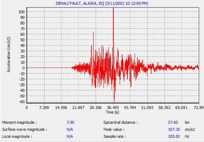
Input earthquake data for dynamic analysis in Plaxis as provided at the fixed end of slope mode
-
In the third phase, the phi-c reduction technique is applied to evaluate the global factor of safety of the model slope considering plastic equilibrium criteria are to be satisfied.

Results and discussions of numerical analysis
The results obtained from the numerical approach and sensitivity analysis are presented in the following sections.
Study of deformed mesh
The generated deformed mesh is shown in Fig. 13. From the arrangement of the mesh, it is observed that the mesh is deformed in a vertical direction under the surcharge loading. As the distance from the surcharge loading increases, the vertical deformation due to the surcharge loading gradually going to be decreased. Also, the maximum horizontal deformation occurs at the sloping side of the slope as shown in the plot.

The plot of deformed mesh due to the loadings (exaggeration factor: 1)
Response of slope due to acceleration
Figure 14a shows the peak acceleration value at different depth of slope at a distance of 6.5 m from AB face (Fig. 10) whereas Fig. 14b presents the acceleration vs time curve of slope at top and bottom surface of the slope after the application of acceleration at the fixed end of the slope. The peak value of applied acceleration is 1.073 m/s2 and the corresponding kh value is 0.1. From the plot, it is seen that the peak value of acceleration increase towards the direction of the surface and at the top surface of the slope it becomes maximum (1.027 m/s2). It is obvious as the soil at the top surface is free to move. It is also seen from the plot at the fixed boundary of the slope there is no acceleration.

Plot of acceleration vs depth a peak value at different depth, b at top and bottom surface
Horizontal and Vertical deformation of the slope
The horizontal deformation and corresponding contour lines are shown in Fig. 15a, b respectively due to the application of the earthquake loading. From the plot, it is seen that the soil at the sloping face displaced at a larger amount indicating slope type of rotational failure of the soil mass. The range of horizontal displacement for slope failure is greater than 22.5 mm. When the displacement contour passes through toe it generates 15 mm displacement and if displacement contour passes through base the related displacement is 12.5 mm or less. On the other hand, Fig. 16a, b shows the variation of vertical displacement and contour lines respectively. From the plot, it is noticed that the maximum vertical deformation occurs just below the top surface of the slope at which point the load is applied. It is also seen that the vertical deformation gradually decreases with the depth and nearly after two-third of the depth, the vertical deformation completely disappears.

Plot of horizontal displacements at β = 20° a Shadings b Contour lines

Plot of vertical displacements β = 20° a Shadings, b Contour lines
Variation of total stress
The variation of total stresses and corresponding contour lines due to the application of earthquake is presented in Fig. 17a, b respectively. From the diagram, it is observed that due to the applied force maximum compressive stresses occur at the bottom middle part of the slope and it gradually decreases towards the top and sloping side of the slope.

The plot of total stresses β = 20° a Shadings, b Contour lines. Horizontal Distance (m)
Verification of the present analysis
A two-dimensional finite element analysis has been performed to compare the present analytical solutions. Table 6 presents the comparison of results obtained by the analytical solution with results obtained from finite element analysis. From Table, it is seen that a good match is observed between the results obtained from analytical solutions and finite element analysis. The comparison of the potential failure surfaces between the analytical approach and numerical analysis are shown in Fig. 18.

Potential failure surface at β = 20°, kh = 0.1, kv = 0, φ = 40°, c/γH = 0.05 and q/γH = 0
According to Fig. 14, the peak ground acceleration found after the numerical analysis is 1.05 m/s2. In the analytical, the applied peak value is given by,
Hence, the PGA value calculated in numerical analysis agrees well with the value obtained in the analytical solution.
Conclusions
An attempt is made to evaluate the factor of safety of soil slope using a pseudo-dynamic limit equilibrium method and considering a log-spiral failure surface. An attempt is also made to compare the analytical solution with the results obtained from the PLAXIS 2D solution. A detailed parametric study is done for the variation of different parameters in the case of both analytical and numerical solutions. It is seen that factor of safety decreases with the increase of horizontal and vertical seismic accelerations, slope angle and surcharge loading. On the other hand, with the increase of soil friction angle and cohesion factor of safety increases. As the increase of depth, the acceleration of the slope decrease and the acceleration at the top surface becomes maximum. It is also observed that maximum horizontal deformation occurs at the sloping side of the slope, whereas slope deformed maximum vertical deformation occurs just below the load is applied. Slope experiences maximum compressive stress at the bottom middle part of the slope. The results obtained from the present analysis are compared with the previous pseudo-static and pseudo-dynamic analyses of slope and found to be a lower value than previous analyses. After optimization, the center of rotation is determined and finally, the initial and final radius are known. Based on those values, the potential failure surface is plotted to show the shape of the slip surface under critical condition and a comparison with the numerical and experimental failure surfaces proves that the logarithmic failure surface is feasible in comparison to linear or circular failure surface. The results as obtained from the present study may be used for stability analysis of slope under seismic loading condition. As a future scope of the work, it is mentioned here that the present suggested analytical methodology can easily be extended for non-homogeneous soil slope even if there are an arbitrary number of non-homogeneous blocks of soil within the failure wedge.
The present methodology uses an analytical method where earthquake forces are considered in an approximate way without writing down the displacement equation under a real dynamic environment which ultimately moves to numerical analysis.
Abbreviations
- a (z,t):
-
Acceleration at depth z with time t
- Q h , Q v :
-
Horizontal and Vertical inertia forces due to seismic acceleration
- b 1 :
-
Width of ith slice
- b 2 :
-
Width of jth slice
- c :
-
Cohesion of soil
- φ :
-
Angle of internal friction of soil
- α :
-
Angle of the base of the vertical slice with horizontal
- ξ:
-
Angle between the length of log-spiral surface and horizontal
- i :
-
Any slice in the zone ADB
- j :
-
Any slice in the zone BDE
- r o :
-
Initial radius of log-spiral curve
- r :
-
Final radius of log-spiral curve
- H :
-
Height of slope
- h :
-
Height of any slice
- W i , W j :
-
Weight of the ith and jth slice respectively
- g :
-
Acceleration due to gravity
- G :
-
Shear modulus of soil
- k h , k v :
-
Intensity of horizontal and vertical seismic acceleration
- q:
-
Load due to surcharge
- t :
-
Any time during vibration (seconds)
- T :
-
Time Period (seconds)
- v s :
-
Shear wave velocity
- v p :
-
Primary wave velocity
- β :
-
Slope angle
- γ :
-
Unit weight of soil
- FOS:
-
Factor of safety
- \(\nu\) :
-
Poisson’s ratio
References
Felleunius W (1936) Calculation of stability of earth dams. Proc. 2nd Congr. Large Dams Washington 4:445–462
Bishop AW (1955) The use of slip circle in the stability analysis of earth slopes. Geotechnique 5(1):7–17
Morgenstern NR, Price VE (1965) The analyses of the stability of general slip surfaces. Geotechnique 15(1):79–93
Spencer E (1967) A method of analysis of the stability of embankments assuming parallel interslice forces. Geotechnique 17(1):11–26
Janbu, N (1954) Applications of composite slip surfaces for stability analysis. In: Proc. of European Conf. on the Stability of Earth Slopes, Stockholm, Sweden, 3, 43–49
Janbu N (1973) Slope stability computations. R C Hirschfeld and S. Poulos eds Wiley, New York pp 47–86
Zhu DY, Lee CF, Jiang HD (2003) Generalised framework of limit equilibrium methods for slope stability analysis. Geotechnique 53(4):377–395
Terzaghi K (1950) Mechanisms of Land Slides Engineering Geology (Berkeley) Volume Geological Society of America
Spencer E (1973) Thrust line criterion in embankment stability analysis. Geotechnique 23(1):85–100
Sarma SK (1979) Stability analysis of embankments and slopes. J Geotech Eng 105(12):1511–1524
Choudhury D, Basu S, Bray J (2007) Behavior of slopes under static and seismic conditions by limit equilibrium method. GSP 161 Embankments Dam and slopes
Koppula SD (1984) Pseudo-static analysis of clay slopes subjected to earthquakes. Geotechnique 34(1):71–79
Leshchinsky D, San KC (1994) Pseudostatic seismic stability of slopes: design charts. J Geotech Eng ASCE 120(9):1514–1532
Ghosh S (2014) Pseudostatic Analysis of Slope considering Circular Rupture Surface. Int J Geotechn Earthquake Eng 5(2):37–43
Hazari S, Ghosh S, Sharma RP (2017) Pseudo-Static Analysis of Slope considering Log Spiral Failure Mechanism. Indian Geotechnical Conference IIT Guwahati India
Newmark N (1965) Effects of earthquakes on dams and embankments. Geotechnique 15(2):139–160
Sarma SK (1973) Stability analysis of embankments and slopes. Geotechnique 23(3):423–433
Ling HI, Leshchinsky D, Mohri Y (1997) Soil slopes under combined horizontal and vertical seismic accelerations. Earthquake Eng Struct Dynam 26(12):1231–1241
Ling HI, Leshchinsky D, Mohri Y (1999) Seismic Analysis of Sliding Wedge: extended Francais–Culmann’s Analysis. Soil Dyn Earthquake Eng 18(5):387–393
Lee J, Liu Q, Park H (2019) Effect of earthquake motion on the permanent displacement of embankment slopes. KSCE J Civ Eng. 23:4174–4189
Steedman RS, Zeng X (1990) The influence of phase on the calculation of pseudo-static earth pressure on a retaining wall. Geotechnique 40(1):103–112
Choudhury D, Nimbalkar S (2005) Seismic passive resistance by pseudo-dynamic metho. Geotechnique 55(9):699–702
Choudhury D, Nimbalkar SS (2006) Pseudo-dynamic approach of seismic active earth pressure behind retaining wall. Geotech Geol Eng 24(5):1103–1113
Nimbalkar SS, Choudhury D (2008) Effects of body waves and soil amplification on seismic earth pressures. J Earthquake Tsunami 2(1):33–52
Ghosh S, Sharma RP (2010) Pseudo-dynamic active response of non-vertical retaining wall supporting c-ɸ backfill. Geotech Geol Eng 28(5):633–641
Ghosh S, Sharma RP (2012) Pseudo-dynamic evaluation of passive response on the back of a retaining wall supporting c-φ backfill. Int J Geomech Geoeng 7(2):115–121
Ghosh S, Saha A (2014) Nonlinear Failure Surface and Pseudodynamic Passive Resistance of Battered - Faced Retaining Wall Supporting c-ɸ Backfill. Int J Geomech 14(3):04014010
Saha A, Ghosh S (2014) Pseudo-dynamic analysis for bearing capacity of foundation resting on c–φ soil. J Geotech Eng 9(4):379–387
Saha A, Ghosh S (2015) Pseudo-dynamic bearing capacity of shallow strip footing resting on c-ɸ soil considering composite failure surface: bearing capacity analysis using pseudo-dynamic method. J Geotech Eng 6(2):12–34
Basha BM, Babu GLS (2011) Reliability assessment of internal stability of reinforced soil structures: a pseudo-dynamic approach. Soil Dyn Earthquake Eng 30(5):336–353
Chanda N, Ghosh S, Pal M (2015) Pseudo-dynamic analysis of slope considering circular rupture surface. J Geotech Eng 10(3):288–296
Xu X, Zhou XP, Huang XC, Xu L (2017) Wedge-Failure Analysis of the Seismic Slope Using the Pseudodynamic Method. Int J Geomech 17(12):04017108
Qin CB, Chian SC (2017) Kinematic analysis of seismic slope stability with a discretization technique and pseudo-dynamic approach: a new perspective. Geotechnique 68(6):492–503
Guha Ray A, Baidya DK (2017) Reliability based pseudo-dynamic analysis of gravity retaining walls. Indian Geotechn J 48:75–584
Hazari S, Sharma RP, Ghosh S (2020) Swedish circle method for pseudo-dynamic analysis of slope considering circular failure mechanism. Geotech Geol Eng. https://doi.org/10.1007/s10706-019-01170-y
. PLAXIS 2D 8.2 [Computer software]. Delft Netherlands Plaxis
. MATLAB R2013a [Computer software]. Matrix Laboratory Software MathWorks Natick MA
Ghosh S, Paul A (2016) Analysis of soil nail excavation considering rayleigh wave with log-spiral failure surface. Int J Geosynth Ground Eng 2:18. https://doi.org/10.1007/s40891-016-0057-3
Pasternack SC, Gao S (1988) Numerical methods in the stability analysis of slopes. Comput Struct 30(3):573–579
Matsui T, San KC (1992) Finite element slope stability analysis by shear strength reduction technique. Soils Found 32(1):59–70
Ugai K, Leshchinsky D (1995) Three dimensional limit equilibrium and finite element analyses: a comparison of results. SoilsFound 35(4):1–7
Duncan JM (1996) State of the art: limit equilibrium and finite element analysis of slopes. J Geotech Eng 122(7):577–596
Griffiths DV, Lane P (1999) Slope stability analysis by finite elements. Geotechnique 49(3):387–403
Lane P, Griffiths DV (2000) Assessment of stability of slopes under drawdown conditions. J Geotech Geoenviron Eng 126(5):443–450
Griffiths DV, Fenton GA (2004) Probabilistic slope stability analysis by finite elements. J Geotech Geoenviron Eng ASCE 130(5):507–518
Hammouri NA, Malkawi AIH, Yamin MMA (2008) Stability analysis of slopes using the finite element method and limiting equilibrium approach. Bull Eng Geol Environ 67(4):471–478
Acknowledgement
This study is funded by Ministry of Human Resource Development.
Author information
Authors and Affiliations
Corresponding author
Additional information
Publisher's Note
Springer Nature remains neutral with regard to jurisdictional claims in published maps and institutional affiliations.
Rights and permissions
Open Access This article is licensed under a Creative Commons Attribution 4.0 International License, which permits use, sharing, adaptation, distribution and reproduction in any medium or format, as long as you give appropriate credit to the original author(s) and the source, provide a link to the Creative Commons licence, and indicate if changes were made. The images or other third party material in this article are included in the article's Creative Commons licence, unless indicated otherwise in a credit line to the material. If material is not included in the article's Creative Commons licence and your intended use is not permitted by statutory regulation or exceeds the permitted use, you will need to obtain permission directly from the copyright holder. To view a copy of this licence, visit http://creativecommons.org/licenses/by/4.0/.
About this article

Cite this article
Hazari, S., Ghosh, S. & Sharma, R.P. Seismic analysis of slope considering log-spiral failure surface with numerical validation. Geo-Engineering 11, 12 (2020). https://doi.org/10.1186/s40703-020-00118-z
Received:
Accepted:
Published:
DOI: https://doi.org/10.1186/s40703-020-00118-z