Wage versus currency devaluation, price pass-through and income distribution: a comparative input–output analysis of the Greek and Italian economies

Abstract

Using input–output data from Symmetric Input–Output Tables for the year 2010 and relevant price models, this paper provides empirical estimations of medium- and long-run effects of wage and currency devaluations on international price competitiveness and income distribution for two ‘PIIGS economies’, i.e. Greece and Italy. The findings reveal certain differentiated socio-technical production conditions in the economies under consideration casting doubt on the effectiveness of demand-switching policy measures implemented in the post-2010 Eurozone economy. At the same time, however, wage devaluation is found to be a comparatively slow and inefficient process to improve international price competitiveness in the medium-run.

1 Introduction

During 2008 and 2009, the so-called PIIGS economies, i.e. Portugal, Ireland, Italy, Greece and Spain, faced serious external and fiscal imbalances. At that time, it was argued by several researchers that although such imbalances were related (to one degree or another) to significant competitiveness divergences in the Eurozone system, exiting the single currency union would lead to vicious circles of currency devaluations, cost-push inflation, lack of capital inflows, monetary financing of deficits and recessions. Implementation of contractionary fiscal and wage devaluation policy measures emerged thus as a possible, although painful, way to tackle the ‘PIIGS crisis’.

Indeed, as for instance De Grauwe and Ji (2016) remark, ‘since 2008–2009 quite dramatic turnarounds of the relative unit labour costs have occurred (internal devaluations) in Ireland, Spain, and Greece, and to a lesser extent in Portugal and Italy. These internal devaluations have come at a great cost in terms of cost output and employment in the debtor countries mainly because the expenditure-reducing effects of these internal devaluations were more intense than the expenditure switching (competitiveness) effects’. (p. 61). In addition, according to the International Labour Organization (2016, pp. 12–13), in 2015 the average real wage rates in Ireland, Italy, Greece and Spain were still below the levels of 2007 (in Greece real wages have dropped by approximately 25% since that year).

On the other hand, however, there were no processes of significant internal revaluations in the creditor Eurozone economies: ‘Thus, one can conclude that at the insistence of the creditor nations, the burden of the adjustments to the imbalances in the Eurozone has been borne almost exclusively by the debtor countries in the periphery. This has created a deflationary bias that explains why the Eurozone has been pulled into a double-dip recession in 2012–2013, and why real GDP has stagnated since 2008, in contrast to what has happened in the non-Euro EU countries and in the USA’. (De Grauwe and Ji 2016, p. 62). Moreover, empirical evidence suggests that, especially in Portugal, Greece and Spain, the possible rebalancing-price competitiveness effects of that ‘internal devaluation strategy’ were also negatively affected by: (1) the increases in profit margins and indirect taxes; and (2) the nominal appreciation of the euro from the second quarter of 2012 to the second quarter of 2014. Thus, it has been argued that the observed ‘improvement in external balances is mainly explained by the collapse of imports in these countries, and this is a consequence of low relative demand and not of the (weak) improvement in competitiveness’. (Uxó et al. 2014, p. 1; also, see Myant et al. 2016; Bilbao-Ubillos and Fernández-Sainz 2018).

At the end of 2014, the Eurozone inflation rate turned negative, while the subsequent announcement of the European Central Bank’ asset purchase program (on 22 January 2015), the so-called Quantitative Easing Program of 1 trillion euros, led to considerable depreciations of the euro against major international currencies. In fact, ‘between early May 2014 and end-May 2015, the euro depreciated by 23% vis-à-vis the US dollar and by 12% in nominal effective terms (against a basket of currencies of 38 major trading partners of the euro area)’. (European Central Bank 2015, p. 11). According to estimates by the European Commission (2015): ‘On average, a 5% depreciation of the euro’s NEER¹ increases import prices by some 4% after 1 year, with most of the impact occurring in just one quarter. By contrast, it takes around three quarters until changes in import prices are passed on to consumer prices and the response is generally small, as final goods prices incorporate substantial shares of domestically produced inputs (retail, transport, marketing costs). Yet, the extent of the response of consumer prices differs slightly across Member States, partly because of different consumption patterns (a high proportion of services in some countries, a high proportion of energy in others). On average, a 5% depreciation of the euro’s NEER leads to an increase in euro area consumer prices of about 0.3% after 1 year. However, as commodities are largely priced in US dollars and the dollar has appreciated strongly, the impact of recent exchange rate changes on prices may be larger than suggested by these estimates. Export prices in the euro area appear to be less responsive to permanent changes in the NEER than import prices. A 5% depreciation of the euro’s NEER lowers export prices in foreign currencies by about 2% after 1 year. The limited pass-through of exchange rate changes to (foreign currency) export prices may be partly explained by offsetting effects from higher imported intermediate input costs and partly by mark-up adjustments. […] [A] 5% depreciation of the euro’s NEER […] may increase real GDP in the euro area by around 0.3% in the first year and another 0.2% in the second year. […] [T]he impact on Member States’ real economies also depends on how strongly export demand responds to changes in relative prices. Empirical evidence suggests that price elasticities differ widely across countries and industries. For example, the price elasticity of Germany’s exports is estimated to be smaller than that of other large Member States (notably Italy and Spain). Through this channel, the depreciation of the euro may support intra-euro area rebalancing’. (pp. 51–52).

All these facts and figures suggest that both medium- and long-run effects of wage and/or exchange rate changes on prices, income distribution and growth should be taken into consideration before the implementation of demand-switching policy measures. Thus, the purpose of the present paper is to provide empirical estimations of the said price and income distribution effects by focusing exclusively on the input–output configurations of Greece and Italy, i.e. two South Eurozone economies that are characterized, however, by different levels and structures of production² and, at the same time, have experienced significantly different rates of wage devaluation. For this purpose, we use:

• 1. Input–output data from the Symmetric Input–Output Tables (SIOTs) for the ‘pre-adjustment’ year of 2010. At the time of this research (September 2016), SΙΟΤs were available for the years 2005 through 2010.

• 2. Input–output price models involving only circulating capital and competitive imports. These models are related to those introduced by Solow (1959), Metcalfe and Steedman (1981) and Katsinos and Mariolis (2012); nevertheless, their particular structures are imposed not only by the purpose (and underlying assumptions) of this paper but also by the available SIOTs, which provide no data on fixed capital stocks and non-competitive imports.

The remainder of the paper is structured as follows. Section 2 outlines the analytic framework. Section 3 presents and evaluates the main empirical results. Finally, Sect. 4 concludes.

2 Method

2.1 Basic assumptions and price equation

Consider an open, linear economy involving only single products, ‘basic’ commodities (in the sense of Sraffa 1960, pp. 7–8), circulating capital and competitive imports. Assume that:

• 1. At least one commodity enters directly into its own production.

• 2. The economy is ‘viable’; namely, the Perron–Frobenius (P–F hereafter) eigenvalue of the ‘irreducible and primitive’ matrix of total input–output coefficients is less than 1.

• 3. Production imports are paid at the beginning of the common production period. Wages are paid at the end of the common production period, and there are no savings out of this income.³

• 4. The input–output coefficients, output levels, nominal profit rates, sectoral net tax rates on gross output (‘taxes less subsidies on products’) and foreign currency prices of the imported commodities are all exogenously given and constant.

Based on these assumptions, we can write⁴

$${\mathbf{p}}^{\text{T}} = ({\mathbf{p}}^{\text{T}} {\mathbf{D}} + E{\mathbf{p}}^{{*{\text{T}}}} {\mathbf{M}} + {\mathbf{p}}^{\text{T}} {\hat{\mathbf{T}}})[{\mathbf{I}} + {\hat{\mathbf{r}}}] + {\mathbf{w}}^{\text{T}} {\hat{\mathbf{L}}}$$

(1)

where ${\mathbf{p}}^{\text{T}} ( > {\mathbf{0}}^{\text{T}} )$ denotes the $1 \times n$ stationary price vector of domestically produced commodities, $E( = 1)$ the single nominal exchange rate, and ${\mathbf{p}}^{{*{\text{T}}}}$ the $1 \times n$ vector of foreign currency prices of the imported commodities, ${\mathbf{p}}^{\text{T}} = E{\mathbf{p}}^{{*{\text{T}}}}$. Furthermore, ${\mathbf{D}} \equiv [d_{ij} ]$, ${\mathbf{M}} \equiv [m_{ij} ]$ denote the $n \times n$ domestic and imported direct input (or Leontief) coefficients matrices, respectively, ${\hat{\mathbf{T}}} \equiv [\tau_{j} ]$ the $n \times n$ diagonal matrix of net tax rates, I the n × n identity matrix, ${\hat{\mathbf{r}}}$ ($r_{j} \ge - 1$ and ${\hat{\mathbf{r}}} \ne {\mathbf{0}}$) the n × n diagonal matrix of the sectoral profit rates, ${\mathbf{w}}^{\text{T}}$($w_{j} > 0$) the $1 \times n$ vector of money wage rates, and ${\hat{\mathbf{L}}}$ ($L_{j} > 0$) the n × n diagonal matrix of direct labour coefficients.

2.2 Wage devaluation

Equation (1) can be rewritten as

$${\mathbf{p}}^{\text{T}} = {\mathbf{p}}^{\text{T}} {\mathbf{F}} + E{\mathbf{m}}^{\text{T}} + {\mathbf{w}}^{\text{T}} {\hat{\mathbf{L}}}$$

(2)

where ${\mathbf{F}} \equiv [{\mathbf{D}} + {\hat{\mathbf{T}}}][{\mathbf{I}} + {\hat{\mathbf{r}}}]$ and ${\mathbf{m}}^{\text{T}} \equiv {\mathbf{p}}^{{*{\text{T}}}} {\mathbf{M}}[{\mathbf{I}} + {\hat{\mathbf{r}}}]$. From Eq. (2), it directly follows that $\lambda_{{{\mathbf{F}}1}} < 1$, since ${\mathbf{p}}^{\text{T}} > {\mathbf{0}}^{\text{T}}$.

In order to estimate the price effect of wage devaluation, we use the following dynamic version of system (2):

$${\mathbf{p}}_{t + 1}^{\text{T}} = {\mathbf{p}}_{t}^{\text{T}} {\mathbf{F}} + E{\mathbf{m}}^{\text{T}} + {\mathbf{w^{{\prime}}}^{\text{T}}} {\hat{\mathbf{L}}},\quad t = 0,1,2, \ldots$$

(3)

where ${\mathbf{p}}_{0}^{\text{T}} = {\mathbf{p}}^{\text{T}}$, ${\mathbf{w^{{\prime}}}^{\text{T}}} \equiv (1 - w){\mathbf{w}}^{\text{T}}$ and $w$ denotes the uniform devaluation rate, $0 < w < 1$. The solution of Eq. (3) is

$${\mathbf{p}}_{t + 1}^{\text{T}} = {\mathbf{p}}_{0}^{\text{T}} {\mathbf{F}}^{t + 1} + (E{\mathbf{m}}^{\text{T}} + {\mathbf{w}}^{{'{\rm T}}} {\hat{\mathbf{L}}})[{\mathbf{F}}^{t} + {\mathbf{F}}^{t - 1} + \cdots + {\mathbf{F}} + {\mathbf{I}}]$$

(4)

From Eqs. (1) and (3), it follows that the initial value of the actual average profit rate is given by

$$\bar{r}_{0} \equiv ({\mathbf{p}}_{0}^{\text{T}} {\mathbf{A}}{\hat{\mathbf{r}}}{\mathbf{x}})({\mathbf{p}}_{0}^{\text{T}} {\mathbf{Ax}})^{ - 1}$$

(5)

where ${\mathbf{A}} \equiv {\mathbf{D}} + {\mathbf{M}} + {\hat{\mathbf{T}}}$ and ${\mathbf{x}}$ ($> {\mathbf{0}}$) denotes the $n \times 1$ vector of the actual gross outputs. The per period average inflation rate is defined as

$$\pi_{t} \equiv ({\mathbf{p}}_{t}^{\text{T}} {\mathbf{x}})({\mathbf{p}}_{t - 1}^{\text{T}} {\mathbf{x}})^{ - 1} - 1,$$

and therefore, the per period average real profit rate could be estimated by (see e.g. Lager 2001)

$$\rho_{t} \equiv (\bar{r}_{0} - \pi_{t} )(1 + \pi_{t} )^{ - 1}$$

(6)

Finally, the international price competitiveness of the economy could be estimated by the following ‘real exchange rate’ index:

$$q_{t} \equiv E_{t} ({\mathbf{p}}_{t}^{\text{T}} {\mathbf{Ex}})^{ - 1}$$

(7)

where ${\mathbf{Ex}}$($\ge {\mathbf{0}}$) denotes the $n \times 1$ vector of actual exports.

From Eqs. (3), (4), (6) and (7), it follows that:

• 1. The price vector tends to ${\mathbf{p}}_{\infty }^{\text{T}} \equiv (E{\mathbf{m}}^{\text{T}} + {\mathbf{w^{{\prime}}}^{\text{T}}} {\hat{\mathbf{L}}})[{\mathbf{I}} - {\mathbf{F}}]^{ - 1}$, since $\lambda_{{{\mathbf{F}}1}} < 1$; that is, ${\mathbf{p}}_{\infty }^{\text{T}} = {\mathbf{p}}_{0}^{\text{T}} - w{\mathbf{w}}^{\text{T}} {\hat{\mathbf{L}}}[{\mathbf{I}} - {\mathbf{F}}]^{ - 1}$ and ${\mathbf{p}}_{\infty }^{\text{T}} > (1 - w){\mathbf{p}}_{0}^{\text{T}}$. The adjustment of the price vector towards its new equilibrium level depends on the magnitudes of $\lambda_{{{\mathbf{F}}1}}$ and $\lambda_{{{\mathbf{F}}1}} \left| {\lambda_{{{\mathbf{F}}k}} } \right|^{ - 1}$. More specifically, the number $- \log \lambda_{{{\mathbf{F}}1}}$ provides a measure for the ‘convergence rate’ of ${\mathbf{p}}_{t + 1}^{\text{T}}$ to ${\mathbf{p}}_{\infty }^{\text{T}}$ (see e.g. Berman and Plemmons 1994, chap. 7), while the number $\lambda_{{{\mathbf{F}}1}} \left| {\lambda_{{{\mathbf{F}}2}} } \right|^{ - 1}$, known as the ‘smallest damping ratio’, can be considered as a lower measure of the intrinsic resilience of ${\mathbf{p}}_{t + 1}^{\text{T}}$ to disturbance (see e.g. Keyfitz and Caswell 2005, pp. 165–175).

• 2. The price-movement is governed by ${\mathbf{w}}^{\text{T}} {\hat{\mathbf{L}}\mathbf{F}}^{t}$, which could be conceived of as the series of ‘dated quantities’ of labour needed for the production of the domestic commodities (see Sraffa 1960, pp. 34–35; Kurz and Salvadori 1995, p. 175), since

  $$w^{ - 1} ({\mathbf{p}}_{t + 1}^{\text{T}} - {\mathbf{p}}_{t}^{\text{T}} ) = - {\mathbf{w}}^{\text{T}} {\hat{\mathbf{L}}\mathbf{F}}^{t}$$

  (8)

  It then follows that the prices of ‘labour-intensive’ commodities tend to, but not necessarily, decrease more than the prices of ‘capital-intensive’ commodities.

  In the extreme (and unrealistic) case where ${\mathbf{F}}$ has rank 1 and, therefore, $\lambda_{{{\mathbf{F}}k}} = 0$ for all $k$, i.e. the damping ratio becomes infinite, Eq. (8) implies that, for $t \ge 1$, the difference vector ${\mathbf{p}}_{t + 1}^{\text{T}} - {\mathbf{p}}_{t}^{\text{T}}$ becomes collinear to the left P–F eigenvector of ${\mathbf{F}}$.

• 3. The average real profit rate first increases and then decreases, tending to $\bar{r}_{0}$, since ${\mathbf{p}}_{t + 1}^{\text{T}} < {\mathbf{p}}_{t}^{\text{T}}$ and $\pi_{t}$ tends to 0.

• 4. The international competitiveness increases and tends to $({\mathbf{p}}_{\infty }^{\text{T}} {\mathbf{Ex}})^{ - 1}$, since $E_{t} = E$.

2.3 Currency devaluation under complete wage indexation

Let ${\mathbf{B}}$, ${\mathbf{B}}^{*}$ be the exogenously given and constant semi-positive $n \times n$ matrices of domestic and imported wage commodities per unit of labour employed, respectively. Then,

$${\mathbf{w}}^{\text{T}} = {\mathbf{p}}^{\text{T}} {\mathbf{B}} + E{\mathbf{p}}^{{*{\text{T}}}} {\mathbf{B}}^{*} ,$$

and therefore, Eq. (1) can be rewritten as

$${\mathbf{p}}^{\text{T}} = {\mathbf{p}}^{\text{T}} {\mathbf{G}} + E{\mathbf{h}}^{\text{T}}$$

(9)

where ${\mathbf{G}} \equiv {\mathbf{F}} + {\mathbf{B}}{\hat{\mathbf{L}}}$ and ${\mathbf{h}}^{\text{T}} \equiv {\mathbf{m}}^{\text{T}} + {\mathbf{p}}^{{*{\text{T}}}} {\mathbf{B}}^{*} {\hat{\mathbf{L}}}$. From Eqs. (2) and (9), it directly follows that $\lambda_{{{\mathbf{F}}1}} < \lambda_{{{\mathbf{G}}1}} < 1$, since ${\mathbf{F}} \le {\mathbf{G}}$ and ${\mathbf{p}}^{\text{T}} > {\mathbf{0}}^{\text{T}}$.

In order to estimate the price effect of currency devaluation, we use the following dynamic version of system (9):

$${\mathbf{p}}_{t + 1}^{\text{T}} = {\mathbf{p}}_{t}^{\text{T}} {\mathbf{G}} + E^{\prime}{\mathbf{h}}^{\text{T}} ,\quad \, t = 0 , 1 , 2 ,\ldots$$

(10)

where ${\mathbf{p}}_{0}^{\text{T}} = {\mathbf{p}}^{\text{T}}$, $E^{\prime} \equiv (1 + \varepsilon )E$ and $\varepsilon$$( > 0)$ denotes the devaluation rate. The solution of Eq. (10) is

$${\mathbf{p}}_{t + 1}^{\text{T}} = {\mathbf{p}}_{0}^{\text{T}} {\mathbf{G}}^{t + 1} + E^{\prime}{\mathbf{h}}^{\text{T}} [{\mathbf{G}}^{t} + {\mathbf{G}}^{t - 1} + \cdots + {\mathbf{G}} + {\mathbf{I}}]$$

(11)

From Eqs. (6), (7), (10) and (11), it follows that:

• 1. The price vector tends to ${\mathbf{p}}_{\infty }^{\text{T}} \equiv E^{\prime}{\mathbf{h}}^{\text{T}} [{\mathbf{I}} - {\mathbf{G}}]^{ - 1}$, since $\lambda_{{{\mathbf{G}}1}} < 1$; that is, ${\mathbf{p}}_{\infty }^{\text{T}} = (1 + \varepsilon ){\mathbf{p}}_{0}^{\text{T}}$. Analogously to the case of the wage devaluation, the price adjustment process depends on the magnitudes of $\lambda_{{{\mathbf{G}}1}}$ and $\lambda_{{{\mathbf{G}}1}} \left| {\lambda_{{{\mathbf{G}}k}} } \right|^{ - 1}$.

• 2. The price-movement is governed by ${\mathbf{h}}^{\text{T}} {\mathbf{G}}^{t}$, which could be conceived of as the series of dated quantities of imported inputs needed for the production of the domestic commodities, since

  $$\varepsilon^{ - 1} ({\mathbf{p}}_{t + 1}^{\text{T}} - {\mathbf{p}}_{t}^{\text{T}} ) = {\mathbf{h}}^{\text{T}} {\mathbf{G}}^{t}$$

  (12)

  It then follows that the prices of ‘imported input-intensive’ commodities tend to, but not necessarily, increase more than the prices of ‘domestic input-intensive’ commodities.

• 3. The average real profit rate first decreases and then increases, tending to $\bar{r}_{0}$, since ${\mathbf{p}}_{t}^{\text{T}} < {\mathbf{p}}_{t + 1}^{\text{T}}$ and $\pi_{t}$ tends to 0.

• 4. The international competitiveness first increases and then decreases, returning to its initial value, since ${\mathbf{p}}_{\infty }^{\text{T}} = (1 + \varepsilon ){\mathbf{p}}_{0}^{\text{T}}$.

2.4 Long-run trade-offs

Now, we assume that the distributive variables ($w_{j}$ or/and $r_{j}$) exhibit stable structures in relative terms. Thus, Eq. (2) can be written as

$${\tilde{\mathbf{p}}}^{\text{T}} = {\tilde{\mathbf{p}}}^{\text{T}} {\mathbf{F}} + \tilde{E}{\mathbf{m}}^{\text{T}} + \tilde{w}(\bar{w}^{ - 1} {\mathbf{w}}^{\text{T}} ){\hat{\mathbf{L}}}$$

or, since $\lambda_{{{\mathbf{F}}1}} < 1$,

$${\tilde{\mathbf{p}}}^{\text{T}} \tilde{E}^{ - 1} = [{\mathbf{m}}^{\text{T}} + (\tilde{w}\tilde{E}^{ - 1} )(\bar{w}^{ - 1} {\mathbf{w}}^{\text{T}} ){\hat{\mathbf{L}}}][{\mathbf{I}} - {\mathbf{F}}]^{ - 1}$$

(13)

where $\bar{w}$ denotes the economy’s actual average wage rate, defined as $\bar{w} \equiv ({\mathbf{w}}^{\text{T}} {\hat{\mathbf{L}}\mathbf{x}})({\mathbf{e}}^{\text{T}} {\hat{\mathbf{L}}\mathbf{x}})^{ - 1}$, and $\tilde{w}$ the ‘overall level’ of wage rates. Furthermore, it is convenient (although not essential) to adopt the actual normalized export vector as the standard of value or numeraire, writing

$${\tilde{\mathbf{p}}}^{\text{T}} {\mathbf{z}} = 1,\,{\mathbf{z}} \equiv ({\mathbf{p}}_{ 0}^{\text{T}} {\mathbf{Ex}})^{ - 1} {\mathbf{Ex}}$$

(14)

Thus, Eqs. (13) and (14) imply

$$\tilde{w} = (1 - \tilde{E}{\mathbf{m}}^{\text{T}} [{\mathbf{I}} - {\mathbf{F}}]^{ - 1} {\mathbf{z}})[(\bar{w}^{ - 1} {\mathbf{w}}^{\text{T}} ){\hat{\mathbf{L}}}[{\mathbf{I}} - {\mathbf{F}}]^{ - 1} {\mathbf{z}}]^{ - 1}$$

(15)

which defines the linear trade-off between ‘the’ wage rate and the exchange rate, measured in terms of the normalized export vector ${\mathbf{z}}$. It is noted that (1) commodity prices are linear functions of $\tilde{E}$; and (2) the straight line defined by Eq. (15) passes through the point: ($\tilde{E} = E = 1$, $\tilde{w} = \bar{w}$), at which ${\tilde{\mathbf{p}}}^{\text{T}} = {\mathbf{p}}_{0}^{\text{T}}$.

Equation (2) can also be written as

$${\tilde{\mathbf{p}}}^{\text{T}} = {\tilde{\mathbf{p}}}^{\text{T}} {\tilde{\mathbf{F}}}(\tilde{r}) + \tilde{E}{\tilde{\mathbf{m}}}(\tilde{r})^{\text{T}} + {\mathbf{w}}^{\text{T}} {\hat{\mathbf{L}}}$$

or, if $\lambda_{{{\tilde{\mathbf{F}}}(\tilde{r})1}} < 1$,

$${\tilde{\mathbf{p}}}^{\text{T}} \tilde{E}^{ - 1} = ({\tilde{\mathbf{m}}}(\tilde{r})^{\text{T}} + \tilde{E}^{ - 1} {\mathbf{w}}^{\text{T}} {\hat{\mathbf{L}}})[{\mathbf{I}} - {\tilde{\mathbf{F}}}(\tilde{r})]^{ - 1}$$

(16)

where ${\tilde{\mathbf{F}}}(\tilde{r}) \equiv [{\mathbf{D}} + {\hat{\mathbf{T}}}][{\mathbf{I}} + \tilde{r}(\bar{r}_{0}^{ - 1} {\hat{\mathbf{r}}})]$, ${\tilde{\mathbf{m}}}(\tilde{r})^{\text{T}} \equiv {\mathbf{p}}^{{*{\text{T}}}} {\mathbf{M}}[{\mathbf{I}} + \tilde{r}(\bar{r}_{0}^{ - 1} {\hat{\mathbf{r}}})]$ and $\tilde{r}$ denotes the overall level of profit rates. Each element in $[{\mathbf{I}} - {\tilde{\mathbf{F}}}(\tilde{r})]^{ - 1}$ is positive and a strictly increasing convex function of $\tilde{r}$, tending to plus infinity as $\lambda_{{{\tilde{\mathbf{F}}}(\tilde{r})1}}$ approaches 1 from below (see e.g. Kurz and Salvadori 1995, p. 116). Thus, Eqs. (14) and (16) imply

$$\tilde{E} = (1 - {\mathbf{w}}^{\text{T}} {\hat{\mathbf{L}}}[{\mathbf{I}} - {\tilde{\mathbf{F}}}(\tilde{r})]^{ - 1} {\mathbf{z}})({\tilde{\mathbf{m}}}(\tilde{r})^{\text{T}} [{\mathbf{I}} - {\tilde{\mathbf{F}}}(\tilde{r})]^{ - 1} {\mathbf{z}})^{ - 1}$$

(17)

which defines the trade-off between the exchange rate and ‘the’ profit rate. It is noted that (1) commodity prices are not necessarily monotonic functions of $\tilde{r}$; and (2) the curve defined by Eq. (17) passes through the point: ($\tilde{r} = \bar{r}_{0}$, $\tilde{E} = E = 1$), at which ${\tilde{\mathbf{p}}}^{\text{T}} = {\mathbf{p}}_{0}^{\text{T}}$.

It will now be clear that, for $\tilde{E} = E = 1$, there is also a trade-off between the wage rate and the profit rate, defined by

$$\tilde{w} = (1 - {\tilde{\mathbf{m}}}(\tilde{r})^{\text{T}} [{\mathbf{I}} - {\tilde{\mathbf{F}}}(\tilde{r})]^{ - 1} {\mathbf{z}})[(\bar{w}^{ - 1} {\mathbf{w}}^{\text{T}} ){\hat{\mathbf{L}}}[{\mathbf{I}} - {\tilde{\mathbf{F}}}(\tilde{r})]^{ - 1} {\mathbf{z}}]^{ - 1}$$

(18)

The curve defined by Eq. (18) passes through the point: ($\tilde{r} = \bar{r}_{0}$,$\tilde{w} = \bar{w}$), at which ${\tilde{\mathbf{p}}}^{\text{T}} = {\mathbf{p}}_{0}^{\text{T}}$.

These three trade-offs yield the loci of all feasible long-run income (re)distributions. Hence, taking also into account Eqs. (13) and (16), it follows that:

• 1. In terms of control system theory, the reciprocal of the functions defined by Eqs. (15), (17) and (18) constitutes ‘transfer functions’ of the dynamic systems defined by Eqs. (3) and (10) (consider Mariolis 2003; Mariolis and Tsoulfidis 2016, pp. 28–29).

• 2. If the wage rate (the profit rate) is held constant, an increase in the exchange rate relative to the wage rate, i.e. an ‘effective currency devaluation’, must reduce the profit rate (the wage rate). As Metcalfe and Steedman (1981) remark, ‘an effective [currency] devaluation […] necessarily reduces at least one of $\tilde{w}$ and $\tilde{r}$. The precise outcome will depend on the proximate forces which determine the distribution of income. In a ‘classical’ world, with the real wage as a datum, the full incidence of an effective [currency] devaluation must fall on the rate of profits. […] [This] conclusion […] may have particularly important implications for the growth rate and long-nm competitive strength of an economy, to the extent that these factors are influenced by the rate of return on invested capital. In a ‘post-Keynesian’ world, where firms can maintain a given rate of profits, the full incidence of an effective devaluation must fall on the real wage rate. Of course, if firms can maintain the profits rate and workers are unwilling to concede any reduction in real wages then, in this impasse, an effective change in the exchange rate is logically impossible (for given ${\mathbf{p}}^{{*{\text{T}}}}$, ${\mathbf{D}}$, ${\mathbf{M}}$, ${\hat{\mathbf{T}}}$, ${\hat{\mathbf{L}}}$). The only consequence of a money devaluation, in this situation, will be an equal proportionate increase in the money wage and in all money prices of domestically produced commodities […]. The literature which explicitly links devaluation to variations in the real wage clearly allows for only one of several possibilities’. (pp. 7–8; using our symbols).

• 3. An effective currency devaluation improves the competitiveness of domestic output, since it cheapens all domestic products relative to all imported commodities.

• 4. Technical progress (i.e. a decrease in any of the elements of ${\mathbf{D}}$, ${\mathbf{M}}$, ${\hat{\mathbf{L}}}$), or a decrease in any foreign import price or net tax rate, necessarily implies that the trade-off curves move outwards from the origin. Hence, the areas under those curves can be conceived of as measures of the economy’s overall performance (see Degasperi and Fredholm 2010).

It should finally be stressed that Metcalfe and Steedman (1981) also provided an explicit integration of the price and quantity sides of the economic system.⁵ Thus, they were able to show that: ‘For given prices and distribution, our analysis of the export-employment multiplier is an entirely traditional (but disaggregated) application of the theory of effective demand. Extra exports produce extra employment in the aggregate. However, it is equally clear that any change in prices or distribution will, in general, change the linkage between employment and the export vector. […] [A]n effective devaluation operates by changing relative prices and the distribution of income, and these considerations immediately suggest that the conventional ‘fix-price’, foreign trade multiplier cannot be readily integrated with the traditional elasticity analysis to deduce the effect[s] of an exchange rate change upon employment [, net outputs, aggregate wages and profits, and trade balance]. […] We can thus offer support both (neither) to those who suggest a positive, effective demand based, relation and (nor) to those who suggest an inverse, supply and demand based, relation between employment levels and real wage rates’. (pp. 15–16).⁶

The hitherto available empirical studies of the matrix multipliers of autonomous demand⁷ (government consumption expenditures, investments and exports) do not take into account neither the underlying income distribution changes nor the possible underutilization of productive capacity (which may result in a non-inverse relationship between the distributive variables⁸). Hence, the estimation of the total multiplier effects for actual economies is a pending issue.

3 Results and discussion

The application of our analytic framework to the SIOTs of the Greek and Italian economies, for the year 2010 (n = 63), gives the following main results⁹:

• 1. Tables 1 and 2 report the estimations of the arithmetic mean values of the dated quantities of direct labour and imported inputs, i.e. ${\mathbf{w}}^{\text{T}} {\hat{\mathbf{L}}\mathbf{F}}^{t}$ and ${\mathbf{h}}^{\text{T}} {\mathbf{G}}^{t}$[see Eqs. (8) and (12)], in the three main sectors of the economies, that is, primary production, industry and services. Furthermore, Tables 3 and 4 report the sectoral compositions of imports and exports. It is noted that the Euclidean angle (measured in degrees) between the total import vectors of the two economies is almost 34.1°, while the relevant figure for the total export vectors is almost 75.6°: these figures further indicate the differences between the import–export structures of the two economies under consideration.

  Table 1 Sectoral dated quantities of direct labour and imported inputs; Greece

  Table 2 Sectoral dated quantities of direct labour and imported inputs; Italy

  Table 3 Sectoral compositions (%) of imports and exports; Greece

  Table 4 Sectoral compositions (%) of imports and exports; Italy

• 2. In a recent empirical study, Aydoğuş et al. (2018) introduce the following cost-push input–output price model (using our symbols):

  $${\mathbf{p}}^{\text{T}} = (E{\mathbf{p}}^{{*{\text{T}}}} {\mathbf{M}} + {\mathbf{w}}^{\text{T}} {\hat{\mathbf{L}}} + {\mathbf{v}}^{\text{T}} )[{\mathbf{I}} - {\mathbf{D}}]^{ - 1}$$

  where ${\mathbf{p}}^{\text{T}}$ ($= E{\mathbf{p}}^{{*{\text{T}}}}$) is identified with ${\mathbf{e}}^{\text{T}}$, and ${\mathbf{v}}^{\text{T}}$ denotes the vector of ‘unit operational surplus (unit capital costs)’, while the unit labour and capital costs, ${\mathbf{w}}^{\text{T}} {\hat{\mathbf{L}}} + {\mathbf{v}}^{\text{T}}$, are assumed to be constant. Thus, they estimate the total effect, both direct and indirect, of the nominal exchange rate change on the stationary commodity prices as: ${\mathbf{e}}^{\text{T}} {\mathbf{M}}[{\mathbf{I}} - {\mathbf{D}}]^{ - 1}$, i.e. as the sums of the column elements of ${\mathbf{M}}[{\mathbf{I}} - {\mathbf{D}}]^{ - 1}$.¹⁰ The calculations are performed for 26 countries (including Italy, for the year 2010, but not Greece) and 27 sectors, using IO tables (from OECD Stan Database, Eurostat, and Izmir Regional Development Agency (IZKA) of Turkey): ‘The estimates presented here should be considered to be upper limits; actual changes in the prices are likely to be lower […]. The results range from 0.07 for USA to 0.34 for Ireland. [For Italy, the result is 0.174.] The average is 0.18; on average, a unit change in the exchange rate causes a 0.18 unit change in the CPI [consumer price index]’. (p. 327).

By applying that approach to our data, we obtained the following results for Greece: 0.138 (primary production), 0.234 (industry), 0.114 (services), 0.161 (total economy) and 0.139 (CPI), while for Italy the results were as follows: 0.112, 0.345, 0.115, 0.203 and 0.170, respectively.¹¹

It should be noted, however, that the sums of the column elements of ${\mathbf{M}}[{\mathbf{I}} - {\mathbf{D}}]^{ - 1}$ coincide with both the vector of share of ‘foreign content (or foreign value added)’ in final demand for domestically produced products (see Hummels et al. 2001) and the vector of ‘total backward leakages’ (see Reis and Rua 2009).

• 3. Figures 1 and 2 (the horizontal axes are plotted in logarithmic scale) display the moduli of the normalized eigenvalues, $\left| {\lambda_{ \bullet i} } \right|\lambda_{ \bullet 1}^{ - 1}$, of the system matrices, $\bullet \equiv {\mathbf{F}} , { }{\mathbf{G}}$. These figures also report the relevant convergence rates, damping ratios and the arithmetic, $AM$, and geometric, $GM$, means of the nonzero non-dominant eigenvalues (as is well known, the $GM$ is more appropriate for detecting the central tendency of an exponential set of numbers).

  Fig. 1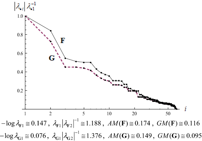

  

  The moduli of the normalized eigenvalues of the system matrices; Greece

  Fig. 2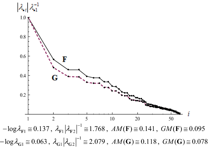

  

  The moduli of the normalized eigenvalues of the system matrices; Italy

• 4. Table 5 reports the estimations of the initial values of the actual average profit rates, $\bar{r}_{0}$ [see Eq. (5)], of the two economies, and their constituent components, i.e. the shares of profits and net taxes (on products) in the net product, the average wage rate, $\bar{w}$, the aggregate labour and capital productivities, and the aggregate capital intensity.

  Table 5 The initial values of the actual average profit rates and their constituent components; Greece and Italy

These figures suggest that the considerable deviation between the values of $\bar{r}_{0}$ in the two economies is directly related to the deviation between the values of the aggregate capital productivities. It should also be noted that, with the exception of six product-industries, the elements of the vector of ‘vertically integrated’ labour coefficients, defined as ${\mathbf{e}}^{\text{T}} {\hat{\mathbf{L}}}[{\mathbf{I}} - ({\mathbf{D}} + {\mathbf{M}})]^{ - 1}$, are greater in the Greek than in the Italian economy; in fact, the ‘mean absolute deviation’ between these vectors is almost 74.4%. By contrast, the P–F eigenvalues of the matrices ${\mathbf{D}}$, ${\mathbf{M}}$ and ${\mathbf{D}} + {\mathbf{M}}$ are greater in the Italian than in the Greek economy; in the case of the Italian economy, these eigenvalues are approximately equal to 0.455, 0.343 and 0.607, respectively, while in the case of the Greek economy, they are approximately equal to 0.380, 0.196 and 0.500, respectively.¹² All these figures are in accordance with those on aggregate labour and capital productivities.

Furthermore, Tables 6 and 7 report the estimations of the evolution of the average inflation rate, $\pi_{t}$, the consumer price index (CPI) and the ‘relative’ average real profit rate, i.e. $\rho_{t} \bar{r}_{0}^{ - 1}$ [see Eq. (6)], $t = 1, \ldots ,4$, for the representative cases where $w = 20\%$ or 30% and $e = 30\%$ or 50%.¹³

Table 6 The evolution of the average inflation rate, CPI and average real profit rate (%); Greece

Table 7 The evolution of the average inflation rate, CPI and average real profit rate (%); Italy

• 5. Tables 8 and 9 report the estimations of the evolution of the international competitiveness of the economies, expressed as $q_{t} q_{0}^{ - 1}$ [see Eq. (7)], $t = 1, \ldots ,3$, for the cases where the devaluation rates are in the range of 20–50%.

  Table 8 The evolution of the international competitiveness (%); Greece

  Table 9 The evolution of the international competitiveness (%); Italy

• 6. Tables 10 and 11 report the long-run effects of the two devaluations on the initial (actual) values of the distributive variables ($\tilde{w} = \bar{w}$, $\tilde{r} = \bar{r}_{0}$; see Table 5). More specifically, in Table 10, the values for the profit rate are estimated by Eq. (18), for w = 20% or 30%, while, in Table 11, the values of the wage and profit rates are estimated by Eqs. (15) and (17), respectively, for e = 30% or 50% (as in Tables 6 and 7). Finally, Table 12 reports the areas under the $\tilde{w} - \tilde{E}$, $\tilde{E} - \tilde{r}$ and $\tilde{w} - \tilde{r}$ curves.¹⁴

  Table 10 The long-run effect of wage devaluation on the profit rate; Greece and Italy

  Table 11 The long-run effects of currency devaluation on the wage and profit rates; Greece and Italy

  Table 12 The areas under the wage-exchange-profit rates curves; Greece and Italy

From these results, it is deduced that:

• 1. In general lines, the shares of dated quantities of labour and, in particular, of imported inputs in the cost of outputs tend to be greater in the Greek than in the Italian economy.

More specifically, in the case of the Greek economy, services is the most labour and export-intensive sector and, at the same time, the less imported input-intensive one, whereas industry is the most imported input and (total) import-intensive sector. Finally, the relatively high indirect dependencies of the primary production sector on both labour and imported inputs, as well as the relatively high direct dependence of industry on labour inputs, are also noticeable (see Tables 1 and 3). Thus, it can be concluded that the international competitiveness effects of wage devaluation tend to be more (less) favourable for the service (for the primary production) sector, while those of currency devaluation tend to be more (less) favourable for the service (for the industry) sector.

In the case of the Italian economy, services is the most labour-intensive sector and, at the same time, the less imported input-intensive one, whereas industry is the most imported input-, import- and export-intensive sector and, at the same time, the less labour-intensive one. Finally, the high dependencies of the primary production sector on both direct labour and indirect imported inputs are also noticeable (see Tables 2 and 4). Thus, it can be concluded that the international competitiveness effects of wage devaluation tend to be more (less) favourable for the service (for the industry) sector, while those of currency devaluation tend to be more (less) favourable for the service (for the industry) sector.

• 2. Regarding the Greek economy and the case of currency devaluation, our aforementioned findings do not differ much from those reported by Katsinos and Mariolis (2012), which are based on the input–output table data for the year 2005 and on different model assumptions. This probably suggests that the structural features of the Greek economy have been shaped well before the emergence of the so-called PIIGS crisis (in this vein, see Mariolis et al. 2018a). Our findings also seem to be compatible with those of empirical studies on the matrix multipliers of autonomous demand for the Greek economy, which conclude that:¹⁵

  • a. The industry sector is heavily dependent on imports and, therefore, diverges considerably from the industry sector in the Eurozone economy.

  • b. The highly import-dependent industries tend to be characterized by low output and employment multipliers and, at the same time, by high import multipliers.

  • c. A well-targeted effective demand management policy could be mainly based on the service sector, and is necessary but not sufficient for resetting the economy on viable paths of recovery. Hence, industrial policy and structural transformation are also needed.

• 3 In both economies, the convergence rate of the wage devaluation process is considerably greater than that of the currency devaluation process, while the damping ratios of the wage devaluation process tend to be less than those of the currency devaluation process (see Figs. 1, 2).¹⁶ These facts are reflected in the evolutions of the average inflation and real profit rates (see Tables 6, 7) and of the international competitiveness of the two economies (see Tables 8, 9). In particular, considering that, as already mentioned, large wage devaluations may not be feasible, the findings suggest, for instance, that a wage devaluation of 30% cannot increase competitiveness by more than 15% (that is, 13.2% in the case of the Greek economy, and 14.5% in the case of the Italian economy). On the other hand, 2 years after a currency devaluation of 50%, competitiveness could remain at least 21% higher than its initial level (that is, 21.4% in the case of the Greek economy, and 25.8% in the case of the Italian economy).

In conclusion, our price pass-through estimations seem not to be in contradiction with the findings reported in some other studies on currency and wage devaluations (using either similar or different frameworks).¹⁷ For instance, as Salvatore (2013) remarks, empirical evidence on large currency devaluations during the turbulent period 1997 (second quarter) to 1999 (third quarter) shows that ‘except for Indonesia, the inflation rate in the [other] Asian countries considered [i.e. Thailand, Korea and Malaysia] was less than one-third of the rate of depreciation of their currencies. In other words, about one-third of the price advantage that these nations received from currency depreciation was wiped out by the resulting [accumulated] inflation. In Indonesia, the rate was 72.5% (49.0/67.6). In Latin America, it was about 20% for Brazil and 46% for Chile. In Mexico, the rate of inflation was almost double the rate of depreciation of its currency’. [p. 513; also, consider the relevant empirical evidence provided by Borensztein and De Gregorio (1999) and Frankel et al. (2012)].

• 4. Both effective wage and currency devaluations imply significant effects on income distribution in the long-run, while the wage rate is more sensitive than the profit rate to currency devaluation (see Tables 10, 11). Finally, the findings suggest a rather mixed picture of the economies’ comparative long-run performance with respect to the two types of devaluations (see Table 12). This probably results from the fact that the Greek economy tends to be characterized by higher levels of sectoral capital productivities, whereas the Italian economy tends to be characterized by higher levels of sectoral labour productivities and shares of foreign content in final demand (or, equivalently, total backward leakages).

4 Conclusions

Using input–output data from the Symmetric Input–Output Tables for the year 2010 and relevant linear price models, this paper estimated the effects of wage and currency devaluations on sectoral price levels and overall levels of income distribution variables for the Greek and Italian economies. It has been detected that:

• 1. The medium-run aggregate competitiveness effects of wage devaluation tend to be similar in the two economies considered, whereas those of currency devaluation are more favourable in the case of the Italian economy. This results from inter-country differences in sectoral (a) export compositions; and (b) dependencies on labour and imported inputs.

• 2. In terms of improving international competitiveness in the medium-run, wage devaluation appears as a slower and less efficient process than currency devaluation.

• 3. Although both devaluations may imply significant effects on income distribution, effective currency devaluation involves a range of alternative distributive regimes. In the long-run, the wage rate responds more strongly than the profit rate with respect to currency devaluation.

• 4. Given the inter-country differences in (a) labour and capital productivities; and (b) shares of foreign content in final demand, there is a rather mixed picture of the economies’ comparative long-run performance with respect to the two types of devaluations.

Our results cast doubt on the ‘horizontal’ policy measures implemented in the post-2010 Eurozone economy and seem to point to the limited effectiveness of both types of devaluations as key levers for the required economic adjustment and recovery. Hence, they rather call for a wider and more flexible strategy framework that includes, on the one hand, an intra-Eurozone industrial, trade and currency depreciation policy and, on the other hand, per country- and sector-specific wage rate changes and demand management policies.

Future research work should use post-2014 input–output data, include the quantity side of the economic system, and estimate the total multiplier effects of wage and exchange rate changes upon employment, net outputs, income distribution, and trade balance for all the Eurozone economies.

Appendices

Appendix 1: Data sources and construction of variables

The available SIOTs describe 65 products and industries. However, all the elements associated with the industry ‘Services provided by extraterritorial organisations and bodies’ are all equal to zero, and therefore, we remove them from our analysis. Moreover, since the labour input in the industry ‘Imputed rents of owner-occupied dwellings’ equals zero, we aggregate it with the industry ‘Real estate activities excluding imputed rent’. Thus, we derive SIOTs that describe 63 industries: three industries belong to ‘Primary production’, twenty-four industries belong to ‘Industry’ (i.e. ‘Mining and quarrying’, ‘Processing products’, ‘Energy’, ‘Water supply and waste disposal’ and ‘Construction’), and thirty-six industries belong to ‘Services’.

The construction of the variables is as follows:

• 1. The price vector, ${\mathbf{p}}$, is identified with the summation vector, ${\mathbf{e}}$, i.e. the physical unit of measurement of each product is that unit which is worth of a monetary unit. (In the present SIOTs, the unit is set to 1 million euro.)

• 2. The matrices of direct input coefficients, ${\mathbf{D}}$ and ${\mathbf{M}}$, and the diagonal matrix of direct labour coefficients, ${\hat{\mathbf{L}}}$, are obtained by dividing element-by-element the relevant inputs in each industry by its gross output (i.e. by its ‘Output at basic prices’, which is directly obtained from the SIOT). The diagonal matrix of net tax rates, ${\hat{\mathbf{T}}}$, is obtained in a similar way.

• 3. The element ‘Wage and salaries’ from the SIOT, which is an element of the ‘Value added at basic prices’ of each industry, is considered as the empirical counterpart of total wages in industry j, W_j. Thus, the money wage rate for each industry is estimated as $w_{j} = W_{j} (L_{j} x_{j} )^{ - 1}$, where $x_{j}$ denotes the gross output of the j th industry.

• 4. The sectoral ‘profit factors’ are estimated from

  $$1 + r_{j} = (1 - w_{j} L_{j} )\left( {\sum\limits_{i = 1}^{n} {d_{ij} } + m_{ij} + \tau_{j} } \right)^{ - 1}$$

• 5. The vector of exports, which is directly obtained from the SIOT, is considered as the empirical counterpart of ${\mathbf{Ex}}$.

• 6. The matrices of domestic, ${\mathbf{B}}$, and imported, ${\mathbf{B}}^{*}$, wage commodities per unit of labour employed are estimated from

  $${\mathbf{B}} = ({\mathbf{p}}^{\text{T}} {\mathbf{c}} + E{\mathbf{p}}^{{*{\text{T}}}} {\mathbf{c}}^{*} )^{ - 1} {\mathbf{cw}}^{\text{T}} = [{\mathbf{e}}^{\text{T}} ({\mathbf{c}} + {\mathbf{c}}^{*} )]^{ - 1} {\mathbf{cw}}^{\text{T}}$$

  and

  $${\mathbf{B}}^{*} = ({\mathbf{p}}^{\text{T}} {\mathbf{c}} + E{\mathbf{p}}^{{*{\text{T}}}} {\mathbf{c}}^{*} )^{ - 1} {\mathbf{c}}^{*} {\mathbf{w}}^{\text{T}} = [{\mathbf{e}}^{\text{T}} ({\mathbf{c}} + {\mathbf{c}}^{*} )]^{ - 1} {\mathbf{c}}^{*} {\mathbf{w}}^{\text{T}}$$

  where ${\mathbf{c}}$, ${\mathbf{c}}^{*}$ denote the vectors of final consumption expenditure by households for domestically produced and imported commodities, respectively, which are directly obtained from the SIOT. Finally, the ‘consumer price index’ (CPI) is estimated as $[{\mathbf{e}}^{\text{T}} ({\mathbf{c}} + {\mathbf{c}}^{*} )]^{ - 1} ({\mathbf{c}} + {\mathbf{c}}^{*} )$.

Appendix 2: The long-run trade-offs for the Greek and Italian economies

The graphs in Figs. 3, 4 and 5 depict the long-run trade-offs in terms of the normalized export vectors of the two economies under consideration. It is noted that, with the exception of one element, the other elements of the vector $(\bar{w}^{ - 1} {\mathbf{w}}^{\text{T}} ){\hat{\mathbf{L}}}[{\mathbf{I}} - {\mathbf{F}}]^{ - 1}$ [see the denominator in Eq. (15)] are greater in the Greek economy than in the Italian economy; in fact, the mean absolute deviation between these vectors is almost 82.3%. On the other hand, the signs of the difference between the vectors ${\mathbf{m}}^{\text{T}} [{\mathbf{I}} - {\mathbf{F}}]^{ - 1}$ [see the numerator in Eq. (15)] are mixed, and the same holds true with respect to the components of the other two curves. Hence, it seems that nothing useful can be said, a priori, about the relative position of the curves. For instance, the graphs in Fig. 6 depict the difference, δ, between the Greek and Italian economies’ scalars $(\bar{w}^{ - 1} {\mathbf{w}}^{\text{T}} ){\hat{\mathbf{L}}}[{\mathbf{I}} - {\tilde{\mathbf{F}}}(\tilde{r})]^{ - 1} {\mathbf{z}}$ [see the denominator in Eq. (18)] as a function of the profit rate (the curve depicted in the second graph is non-monotonic).

Fig. 3

The wage-exchange rates trade-off; Greek and Italian economies

Fig. 4

The exchange-profit rates trade-off; Greek and Italian economies

Fig. 5

The wage-profit rates trade-off; Greek and Italian economies

Fig. 6

The difference between the denominator components of the wage-profit rates trade-off as a function of the profit rate; Greek and Italian economies

References

Angelini E, Dieppe A, Pierluigi B (2015) Modelling internal devaluation experiences in Europe: rational or learning agents? J Macroecon 43:81–92
Aydoğuş O, Değer Ç, Çalışkan ET, Günal GG (2018) An input–output model of exchange-rate pass-through. Econ Syst Res 30(3):323–336
Bahmani-Oskooee M, Hegerty SW, Kutan AM (2008) Do nominal devaluations lead to real devaluations? Evidence from 89 countries. Int Rev Econ Finance 17(4):644–670
Berman A, Plemmons RJ (1994) Nonnegative matrices in the mathematical sciences. Society for Industrial and Applied Mathematics, Philadelphia
Bhaduri A, Marglin S (1990) Unemployment and the real wage rate: the economic basis for contesting political ideologies. Camb J Econ 14(4):375–393
Bilbao-Ubillos J, Fernández-Sainz A (2018) A critical approach to wage devaluation: the case of Spanish economic recovery. Soc Sci J. https://doi.org/10.1016/j.soscij.2018.05.006 (in press)
Blecker RA (2011) Open economy models of growth and distribution. In: Hein E, Stockhammer E (eds) A modern guide to Keynesian macroeconomics and economic policies. UK and Northampton, MA, Edward Elgar, Cheltenham, pp 215–239
Borensztein E, De Gregorio J (1999) Devaluation and inflation after currency crises. International Monetary Fund, Mimeo, New York
Brancaccio E, Garbellini N (2015) Currency regime crises, real wages, functional income distribution and production. Eur J Econ Econ Polic Interv 12(3):255–276
Burstein A, Eichenbaum M, Rebelo S (2005) Large devaluations and the real exchange rate. J Polit Econ 113(4):742–784
Ciccarone G, Saltari E (2015) Cyclical downturn or structural disease? The decline of the Italian economy in the last twenty years. J Mod Ital Stud 20(2):228–244
Commission European (2015) European economic forecast. Winter 2015. European Commission. Directorate-General for Economic and Financial Affairs, Brussels
De Grauwe P, Holvoet C (1978) On the effectiveness of a devaluation in the E.C.-countries. Tijdschrift voor Economie en Management 23(1):67–82
De Grauwe P, Ji Y (2016) Crisis management and economic growth in the Eurozone. In: Caselli F, Centeno M, Tavares J (eds) After the crisis. Reform, recovery, and growth in Europe. Oxford University Press, Oxford, pp 46–72
Degasperi M, Fredholm T (2010) Productivity accounting based on production prices. Metroeconomica 61(2):267–281
Donayre L, Panovska I (2016) State-dependent exchange rate pass-through behavior. J Int Money Finance 64:170–195
European Central Bank (2015) The international role of the euro. European Central Bank, Frankfurt am Main
Ferretti F (2008) Patterns of technical change: a geometrical analysis using the wage-profit rate schedule. Int Rev Appl Econ 22(5):565–583
Frankel JA, Parsley D, Wei S-J (2012) Slow pass-through around the world: A new import for developing countries? Open Econ Rev 23(2):213–251
Hummels D, Ishii J, Yi K-M (2001) The nature and growth of vertical specialization in world trade. J Int Econ 54(1):75–96
International Labour Organization (2016) Global wage report 2016/2017. Wage inequality in the workplace. International Labour Office, Geneva
Katsinos A, Mariolis T (2012) Switch to devalued drachma and cost-push inflation: a simple input–output approach to the Greek case. Mod Econ 3(2):164–170
Keyfitz N, Caswell H (2005) Applied mathematical demography, 3rd edn. Springer, New York
Krugman P, Taylor L (1978) Contractionary effects of devaluation. J Int Econ 8(3):445–456
Kurz HD (1990) Technical change growth and distribution: a steady-state approach to ‘unsteady’ growth. In: Kurz HD (ed) Capital, distribution and effective demand. Studies in the ‘classical’ approach to economic theory. Polity Press, Cambridge, pp 211–239
Kurz HD, Salvadori N (1995) Theory of production. A long-period analysis. Cambridge University Press, Cambridge
Lager C (2001) A note on non-stationary prices. Metroeconomica 52(3):297–300
Mariolis T (2003) Controllability, observability, regularity, and the so-called problem of transforming values into prices of production. Asian Afr J Econ Econom 3(2):113–127
Mariolis T (2008) Pure joint production, income distribution, employment and the exchange rate. Metroeconomica 59(4):656–665
Mariolis T (2013) Currency devaluation, external finance and economic growth: a note on the Greek case. Soc Cohes Dev 8(1):59–64
Mariolis T, Soklis G (2015) The Sraffian multiplier for the Greek economy: evidence from the supply and use table for the year 2010, Centre of Planning and Economic Research, Discussion Paper No 142, June. http://www.kepe.gr/index.php/el/erevna/dimosieyseis/ergasies-gia-sizitise-el/item/2735-dp_142. Accessed 25 Mar 2016
Mariolis T, Soklis G (2018) The static Sraffian multiplier for the Greek economy: evidence from the supply and use table for the year 2010. Rev Keynes Econ 6(1):114–147
Mariolis T, Tsoulfidis L (2016) Modern classical economics and reality: a spectral analysis of the theory of value and distribution. Springer, Tokyo
Mariolis T, Tsoulfidis L (2018) Less is more: capital theory and almost irregular-uncontrollable actual economies. Contrib Polit Econ 37(1):65–88
Mariolis T, Leriou E, Soklis G (2018a) Dissecting the input–output structure of the Greek economy 2005–2010. Economia Internazionale/International Economics (forthcoming)
Mariolis T, Ntemiroglou N, Soklis G (2018b) The static demand multipliers in a joint production framework: comparative findings for the Greek, Spanish and Eurozone economies. J Econ Struct 7:18. https://doi.org/10.1186/s40008-018-0116-0
Metcalfe JS, Steedman I (1981) Some long-run theory of employment, income distribution and the exchange rate. Manch School 49(1):1–20
Myant M, Theodoropoulou S, Piasna A (eds) (2016) Unemployment, internal devaluation and labour market deregulation in Europe. European Trade Union Institute (ETUI), Brussels
Ntemiroglou N (2016) The Sraffian multiplier and the key-commodities for the Greek economy: evidence from the input–output tables for the period 2000–2010. Bull Polit Econ 10(1):1–24
Onaran Ö, Galanis G (2012) Is aggregate demand wage-led or profit-led? Na-tional and global effects, Conditions of Work and Employment Series No. 40, Ge-neva: International Labour Office
Reis H, Rua A (2009) An input–output analysis: Linkages versus leakages. Int Econ J 23(4):527–544
Ribeiro RSM, McCombie JSL, Lima GT (2017) Some unpleasant currency-devaluation arithmetic in a post Keynesian macromodel. J Post Keynes Econ 40(2):145–167
Salvatore D (2013) International economics, Eleventh edn. Wiley, New York
Solow RM (1959) Competitive valuation in a dynamic input–output system. Econometrica 27(1):30–53
Sraffa P (1960) Production of commodities by means of commodities. Prelude to a critique of economic theory. Cambridge University Press, Cambridge
Steedman I (1977) Marx after Sraffa. New Left Books, London
Steedman I (1985) Joint production and technical progress. Polit Econ Stud Surpl Approach 1(1):127–138
Tarancón M-A, Gutiérrez-Pedrero M-J, Callejas FE, Martínez-Rodríguez I (2018) Verifying the relation between labor productivity and productive efficiency by means of the properties of the input–output matrices. The European case. Int J Prod Econ 195:54–65
Uxó J, Paúl J, Febrero E (2014) Internal devaluation in the European periphery: The story of a failure, Working Papers DT 2014/2, Albacete, University of Castilla—La Mancha
Authors’ contributions
Authors TM, NR and AK have equally contributed to designing the research, the process of data collection and calculation as well as to writing the manuscript. All authors have read and approved the final manuscript.
Acknowledgements
We are grateful to an anonymous referee of this journal for helpful comments and suggestions. Earlier versions of this paper were presented at a Workshop of the ‘Study Group on Sraffian Economics’ at the Panteion University, in November 2016, and at the ‘2nd International Scientific Conference: Reconstruction of Production in Greece. Economic Crisis and Growth Perspectives’, Technological and Education Institute of Central Macedonia, Serres, Greece, 5–6 May 2017: we would like to thank Eirini Leriou, Nikolaos Ntemiroglou, Maria Pantzartzidou, and George Soklis for very helpful comments and suggestions.
Competing interests
The authors declare that they have no competing interests.
Availability of data and materials
The Symmetric Input–Output Tables (SIOTs) and the corresponding sectoral levels of employment are provided via the Hellenic Statistical Authority, Italian National Institute of Statistics, and Eurostat websites: http://www.statistics.gr/en/statistics/-/publication/SEL38/2010; http://dati.istat.it/?lang=en&SubSessionId=7e7a1f62-9daa-4cc1-919b-6479cb641095; and http://ec.europa.eu/eurostat/web/esa-supply-use-input-tables/data/workbooks (accessed 6 September 2016). Until now, the most recent SIOTs are those for the year 2010: https://ec.europa.eu/eurostat/web/esa-supply-use-input-tables/data/database (accessed 9 October 2018).
Funding
Not applicable.
Publisher’s Note
Springer Nature remains neutral with regard to jurisdictional claims in published maps and institutional affiliations.
Author information
Authors and Affiliations
Corresponding author