
Abstract
Connected and Automated Vehicle (CAV) is a transformative technology that has great potential to improve urban traffic and driving safety. Electric Vehicle (EV) is becoming the key subject of next-generation CAVs by virtue of its advantages in energy saving. Due to the limited endurance and computing capacity of EVs, it is challenging to meet the surging demand for computing-intensive and delay-sensitive in-vehicle intelligent applications. Therefore, computation offloading has been employed to extend a single vehicle’s computing capacity. Although various offloading strategies have been proposed to achieve good computing performace in the Vehicular Edge Computing (VEC) environment, it remains challenging to jointly optimize the offloading failure rate and the total energy consumption of the offloading process. To address this challenge, in this paper, we establish a computation offloading model based on Markov Decision Process (MDP), taking into consideration task dependencies, vehicle mobility, and different computing resources for task offloading. We then design a computation offloading strategy based on deep reinforcement learning, and leverage the Deep Q-Network based on Simulated Annealing (SA-DQN) algorithm to optimize the joint objectives. Experimental results show that the proposed strategy effectively reduces the offloading failure rate and the total energy consumption for application offloading.
Introduction
With the development of artificial intelligence technology, mobile communication technology and sensor technology, the design requirements of vehicles are no longer limited to the driving function. Vehicles are gradually transformed into an intelligent, interconnected and autonomous driving system, namely, Connected and Autonomous Vehicle (CAV)[1]. The rapid increase of vehicles on the road makes traffic accidents, traffic congestion and automobile exhaust pollution become increasingly prominent. A report of the World Health Organization (WHO) pointed out that more than 1.35 million people die in traffic accidents per year [2]. By sharing information with the infrastructure and neighboring vehicles, CAVs can perceive the surrounding environment more comprehensively [3], effectively reducing traffic accidents caused by human error and alleviating traffic congestion. Electric Vehicle (EV)[4], with its advantages in energy saving, is becoming the key subject in the next generation of CAVs. Its electricity can be generated from various renewable energy sources, such as solar energy, wind energy, and geothermal energy, etc [5]. This will greatly reduce the environmental pollution caused by automobile exhaust emissions.
The development of CAV technology has given birth to a series of computing-intensive and delay-sensitive in-vehicle intelligent applications [6], e.g., autonomous driving [7], augmented reality [8], etc. They typically require large amounts of computing resources. But it is challenging for vehicles to meet the surging demand for such emerging applications, due to the limited endurance and computing capacity of vehicles. In recent years, computation offloading has been employed to extend a single vehicle’s computing capacity. The computation offloading methods, based on traditional cloud computing platforms [9], offload computing tasks to cloud computing centers with powerful computing capabilities, effectively alleviating the computing burden on vehicles. However, due to the long transmission distance between vehicles and cloud computing centers, it will not only cause serious service delays, but also lead to huge energy consumption, which can not meet the needs of in-vehicle intelligent applications [10].
To address the above challenges, a new networking paradigm, Vehicular Edge Computing (VEC), has been proposed. VEC deploys Mobile Edge Computing (MEC) servers with computing and storage capabilities in Roadside Units (RSU). This enables CAV applications to be either processed in the vehicles locally, or offloaded to other cooperative vehicles or RSUs within the communication range for processing. This paradigm opens up new challenges on how to manage offloading to keep the offloading failure rate and overall energy consumption low. (1) Offloading failure rate could be impacted by the application execution time and the communication link established between the vehicle and the offloading targets. If the offloaded tasks can not complete within the application’s tolerance time, the offloading fails; if the communication link is broken during the offloading process, the offloading fails. This requires that the offloading strategy should minimize the overall application execution time, and minimize the communication interruption by taking into consideration the vehicle’s continuous movements. (2) Energy consumption also plays an important role in offloading [11, 12]. Both communication and task execution consumes vehicle’s energy. An offloading strategy that can minimize the energy consumption would benefit vehicle’s endurance. Therefore, different offloading strategies can impact both objectives simultaneously, potentially in opposite directions. This necessitates the joint optimization of the two objectives.
Researchers have done a considerable amount of work on CAV computation offloading strategy in the VEC environment. Table 1 lists a group of existing research work, where we mark the objectives, conditions and offloading schemes that are considered for each approach. As we can see, they have the following limitations.
-
1
The optimization objective mainly focused on either execution delay [13, 14] or energy consumption [15, 16], instead of the joint optimization of offloading failure rate and energy consumption [17, 18].
Table 1 Comparison of existing approaches and our approach (✓indicates the corresponding item is considered in the technique) -
2
Most work only considered computation offloading strategy in the static environment [19–21], instead of dynamic offloading strategy with the change of vehicle positions in different time slots.
-
3
They mostly aimed at computation offloading of independent tasks [22, 23], i.e., no data dependency among tasks of an application.
-
4
Most work only considered offloading tasks to RSUs or processing tasks directly on On-Board Unit (OBU) [24, 25], without utilizing the idle computing resources of cooperative vehicles.
To address the above limitations, our work establishes a new computation offloading model, which takes into consideration task dependencies, vehicle mobility, and different computing resources to offload tasks to. Our goal is to jointly optimize the objectives offloading failure rate and energy consumption. To this end, our work employs Deep Reinforcement Learning (DRL), which excels at resolving the dimension disaster problem existed in the traditional reinforcement learning methods [26, 27]. More specifically, our work designs an efficient computation offloading strategy based on Deep Q-Network Based on Simulated Annealing (SA-DQN) algorithm in the VEC environment.
The main contributions of this paper are as follows.
-
A new computation offloading model for CAV applications in the VEC environment is established based on Markov Decision Process (MDP). Since the computation tasks from application decomposition can be processed locally, offloaded to RSUs or cooperative vehicles, the model introduces task queues in vehicles and RSUs to model the task transmission and processing. Moreover, vehicle mobility and temporal dependency among tasks are also considered in the model.
-
The work designs a computation offloading strategy based on deep reinforcement learning, and leverages the SA-DQN algorithm to optimize the joint objectives.
-
The proposed computation offloading strategy is evaluated using real vehicle trajectories. The simulation results show that the proposed strategy can effectively reduce the offloading failure rate and the total energy consumption.
The rest of this paper is organized as follows. Section II introduces the related work of computation offloading in VEC. Section III formally defines the computation offloading problem of CAV applications and the optimization goal, and analyzes the computation offloading process using an example. Section IV proposes the computation offloading strategy based on DRL, and designs the SA-DQN algorithm for the computation offloading strategy. Section V presents and analyzes the experimental results, as well as the performance differences between SA-DQN algorithm and traditional reinforcement learning algorithms. Section VI summarizes this work and looks into future work.
Related work
As shown in Table 1, there have been a wide range of research work on CAV application offloading strategy with different objectives, conditions and offloading schemes. Most existing studies focused on the optimization of either execution delay or energy consumption, but rarely consider joint optimization of execution delay and energy consumption. Wu et al. [13] proposed an optimal task offloading approach using 802.11p as the transmission protocol of inter vehicle communication, in which transmission delay and computation delay are considered to maximize the long-term return of the system. Although a large number of experimental results show that the proposed optimization approach has good performance, the optimization of energy consumption is not considered in this study. Zhang et al. [14] proposed an effective combined prediction mode degradation approach considering the computation task execution time and vehicle mobility. Although the simulation results show that the approach greatly reduces the cost and improves the task transmission efficiency, it does not consider the energy consumption of communication and processing. Jang et al. [15] considered the change of communication environment, jointly optimized the offloading ratio of multiple vehicles, and optimized the total energy consumption of vehicles under the delay constraint. Although the proposed energy-saving offloading strategy significantly reduces the total vehicle energy consumption, it does not consider the processing energy consumption of the computing node. Pu et al. [16] designed an online task scheduling algorithm to minimize the energy consumption of vehicles in the network for multi-vehicle and multi-task offloading problem. Simulation results show that the proposed framework has excellent performance. Wang et al. [17] proposed a dynamic reinforcement learning scheduling algorithm to solve the offloading decision problem. Although the experimental results show that the performance of the proposed algorithm is better than other benchmark algorithms, the offloading of dependent tasks is not considered. Khayyat et al. [18] proposed a distributed deep learning algorithm to optimize the delay and energy consumption. The simulation results show that the algorithm has faster convergence speed.
Some research work only focused on independent task offloading in the VEC environment. Dai et al. [22] proposed a method based on utility table learning, which verified the effectiveness and scalability of the method in various scenarios. The work considers both cloud computing and edge computing platform to offload tasks. Ke et al. [23] proposed a computation offloading method based on deep reinforcement learning in the dynamic environment.
Some studies only considered offloading tasks to RSU or processing tasks locally. Han et al. [24] established a MDP model for the problem, and optimized the offloading strategy with deep reinforcement learning. Although the study considers the change of vehicle’s position in different time slots, it does not make full use of cooperative vehicle resources. Dai et al. [25] transformed the load balancing and offloading problem into an integer non-linear programming problem to maximize the system utility. Experiments show that the strategy is significantly better than the benchmark strategy in terms of system utility. Although the mobility of vehicles is considered in this study, the offloading mode does not consider offloading tasks to cooperative vehicles.
Some studies did not consider the change of vehicle positions in different time slots. Xu et al. [19] proposed an adaptive computation offloading method to optimize the delay of task offloading and resource utilization. Experimental results show the effectiveness of this method. Liu et al. [20] offloaded multiple vehicle applications to RSU, divided each application into multiple tasks with task dependencies, and proposed an efficient task scheduling algorithm to minimize the average completion time of multiple applications. This work divides the application into several tasks to effectively reduce the completion time of application. Guo et al. [21] introduced Fiber-Wireless (FI-WI) integration to enhance the coexistence of VEC network and remote cloud, and proposed two task offloading approaches. The experimental results show that the proposed approaches have advantages in reducing the task processing delay.
Problem definition and analysis
In this section, we first define the problem by modeling the network, application, communication and computation, then analyze an example of the proposed model.
Problem definition
Network model
The VEC network model is shown in Fig. 1. The vehicles are categorized into Task Vehicle (TaV) and Service Vehicle (SeV) [28]. Both are equipped with OBU, and hence they have certain computing capability. TaV is the user of applications, which can be offloaded to SeVs after application decomposition to utilize the computing resources of cooperative vehicles in the neighborhood. There are fixed RSUs deployed on the roadside. Each RSU is equipped with an MEC server, which is integrated with wired connection [29]. They also have certain computing capability. SeVs and RSUs are referred to as Service Nodes (SNs)[30].

VEC network model
In the VEC network model, there are m RSUs {α1,α2,...,αm}, one TaV β1, and n SeVs {γ1,γ2,...,γn}. The coverage radiuses of RSUs are {r1,r2,...,rm}, respectively, and the communication radius of a vehicle is rv. TaV can not only offload computation tasks to RSUs by Vehicle to Infrastructure (V2I) communication, but also to SeVs by Vehicle to Vehicle (V2V) communication. The two offloading schemes are referred to as remote offloading.
To better describe the generation, transmission and processing process of CAV applications, we divide the vehicle travel time into t time slots, with each slot of length ε. In each time slot, the VEC system is quasi-static; that is, the relative position of the vehicle and the wireless channel state are stable, while they may change across different time slots [31].
Application model
Most CAV applications use algorithms based on computer vision or deep learning to process a large amount of data collected by on-board sensors (cameras, radars, etc). CAV local applications and various third-party applications are usually computation-intensive or delay-sensitive applications. They typically need to use a lot of computing resources to process real-time data to meet the requirements of low execution delay [32].
The OBU on CAVs with limited computing resources cannot meet the requirements of applications. Therefore, to fully utilize the computing resources of RSUs and SeVs within CAV’s communication range, CAV applications are decomposed into multiple smaller tasks, potentially with dependecies among them. Let’s assume there are z different CAV applications, and each of them can be generated with probability 1/z in each time slot. As shown in Fig. 2, each CAV application can be decomposed to multiple tasks, denoted as \(\boldsymbol {A}_{i} \buildrel \Delta \over = \{ \boldsymbol {G}_{i},{l_{i}} \}(i \in \{ 1,2,...,z\})\), where Gi is the temporal dependency of decomposed tasks and li is the tolerance time for the i-th application. Specifically, the temporal dependency of tasks is represented by a directed acyclic graph (DAG) Gi=〈Ni,Ei〉, where \(\boldsymbol {N}_{i} = \left \{ \boldsymbol {T}_{1}^{i},\boldsymbol {T}_{2}^{i},...,\boldsymbol {T}_{\left | {\boldsymbol {N}_{i}} \right |}^{i}\right \} \) is the set of decomposed tasks, and \(\boldsymbol {E}_{i} = \left \{e_{u,v}^{i} | f\left (e_{u,v}^{i}\right)=1, 1 \le u,v \le \left | {{\boldsymbol {N}_{i}}} \right |, u \ne v\right \} \) is the set of direct edges representing temporal dependency of tasks. \(f\left (e_{u,v}^{i}\right)=1\) indicates there is a directed edge \(\boldsymbol {T}_{u}^{i} \rightarrow \boldsymbol {T}_{v}^{i}\), while \(f\left (e_{u,v}^{i}\right)=0\) indicates there is no edge. \(\boldsymbol {T}_{u}^{i}\) is called the direct predecessor task of \(\boldsymbol {T}_{v}^{i}\). The direct predecessor task \(\boldsymbol {T}_{u}^{i}\) must be completed before \(\boldsymbol {T}_{v}^{i}\) can be processed. The set of direct predecessors of a task can be denoted as \(\boldsymbol {R}_{v}^{i} = \left \{ \boldsymbol {T}_{u}^{i} | f\left (e_{u,v}^{i}\right)=1, 1 \le u,v \le \left | {{\boldsymbol {N}_{i}}} \right |, u \ne v\right \} \). The task \(\boldsymbol {T}_{v}^{i}\) can not be processed until all tasks in the set of direct predecessors \(\boldsymbol {R}_{v}^{i}\) have been completed. Tasks without any direct predecessor are called entry task, while tasks without any direct successor are called exit task. Moreover, each decomposed task can be represented as \(\boldsymbol {T}_{u}^{i} \buildrel \Delta \over = \left \{ u, Deep\left (\boldsymbol {T}_{u}^{i}\right), d_{u}^{i} \right \}(u \in \{ 1,2,...,\left | {\boldsymbol {N}_{i}} \right |\}\), where u is the decomposed task index, \(Deep\left (\boldsymbol {T}_{u}^{i}\right)\) is the task depth defined by Eq. (1), and \(d_{u}^{i}\) is the task data size.

Decomposition model of CAV’s application
Task queue model
The task queue model is illustrated in Fig. 3. Considering the transmission and processing of task data, we denote a task queue on TaV/SeV as Qt/ Qs, while a task queue on RSUs as Qr. Each task queue holds the tasks from the decomposition of CAV applications. Tasks in the task queue are sorted by task depth first and then by task number in the ascending order.

Task queue model
For the task queue Qt, we have the following definitions:
-
i)
Qt holds the tasks decomposed from TaV applications;
-
ii)
TaV can only transmit or process task data at the head of Qt.
For the task queues Qs and Qr, we have the following definitions:
-
i)
Qs and Qr hold the tasks transmitted by TaV;
-
ii)
SeVs can only process task data at the head of Qs and RSUs can only process task data at the head of Qr.
Communication model
TaV can communicate with SNs to transmit task data at the head of Qt. We define channel bandwidth as B, transmission power of TaV as ptr, channel fading coefficient as h, Gaussian white noise power as χ and path loss exponent as ϖ.
In the i-th time slot, the transmission rate from TaV to SN j is expressed as
where \(\Phi _{i,j}^{SN}\) is the distance between TaV and SN j, defined by
where \(x_{i}^{tav}\) and \(y_{i}^{tav}\) are the two-dimensional coordinates of TaV in the i-th time slot, \(x_{i,j}^{SN{\mathrm {s}}}\) and \(y_{i,j}^{SN{\mathrm {s}}}\) is the two-dimensional coordinates of SN j in the i-th time slot.
In the i-th time slot, only when the distance between TaV and the SN j is within the coverage radius of SN, the task data can be transmitted. If TaV transmits task data to the SN j, the amount of task data transmitted can be expressed as
the data transmission between TaV and SN j will cause energy consumption, which can be expressed as
Computation model
TaV can either transmit the task at the head of Qt to SNs, or process the task locally. SNs only process the task at the head of task queue locally.
The computation model includes two parts: tasks processed by TaV and tasks processed by SNs.
-
a)
Tasks processed by TaV. The power consumption of TaV processing tasks locally is expressed as
$$\begin{array}{@{}rcl@{}} {p^{tav}} = {\kappa_{{tav}}}{({f^{tav}})^{3}} \end{array} $$(6)where κtav is the effective switched capacitance coefficient related to the chip architecture in vehicle [33], and ftav is the local computing capacity of the TaV (i.e., the CPU frequency in cycles/sec). TaV processing tasks will consume a certain amount of energy, expressed as
$$\begin{array}{@{}rcl@{}} \delta_{{tav}}^{process} = {p^{tav}}\varepsilon = {\kappa_{{tav}}}{({f^{tav}})^{3}}\varepsilon \end{array} $$(7)The data size that TaV can process in a time slot is given by
$$\begin{array}{@{}rcl@{}} {d^{tav}} = {{{f^{tav}}\varepsilon} \over c} \end{array} $$(8)where c is the processing density of task data (in CPU cycles/bit).
-
b)
Tasks processed by SNs. The power consumption of SN i processing locally is expressed as
$$\begin{array}{@{}rcl@{}} p_{i}^{SN} = {\kappa_{i}}{\left(f_{i}^{SN}\right)^{3}} \end{array} $$(9)where κi is the effective switched capacitance coefficient related to the chip architecture in SN i. \(f_{i}^{SN}\) is the processing capability of SN i. SNs processing tasks will consume a certain amount of energy, expressed as
$$\begin{array}{@{}rcl@{}} \delta_{i}^{SN} = p_{i}^{SN}\varepsilon = {\kappa_{i}}{(f_{i}^{SN})^{3}}\varepsilon \end{array} $$(10)The data size that SN i can process in a time slot is given by
$$\begin{array}{@{}rcl@{}} d_{i}^{SN} = {{f_{i}^{SN}\varepsilon} \over c} \end{array} $$(11)
In a time slot, TaV can process the task data locally or offload the task to the SNs within the communication range. The offloading decision adopted by TaV can be represented by the 0-1 decision variable as shown in Eq. (12). νi indicates whether TaV processes task data locally in the i-th time slot, and \(o_{j}^{i}\) indicates whether TaV offloads task to SN j in the i-th time slot. SNs process a task only when it is at the head of task queue. \(\theta _{j}^{i}\) indicates whether SN j processes task data in the i-th time slot. β and ζ are the weight coefficients of execution delay and energy consumption respectively, where β+ζ=1.
where faili is offloading failure penalty in the i-th time slot, expressed as
where \(\boldsymbol {D}_{i}^{loss}\) is the data size set of the offloading failed tasks (unprocessed tasks belonged to offloading failed applications in task queues), \(d_{i,j}^{loss}\) is data size of j-th offloading failed task in i-th time slot.
There are two cases that can lead to application offloading failure:
-
1
While the SNs are receiving task data, distance between TaV and SNs is out of the communication range during data transmission.
-
2
The completion time of application is greater than its tolerance time.
In Eq. (12), \(\delta _{i}^{tav}\) is the energy consumption caused by TaV processing tasks, given by
\(\delta _{i}^{tSN}\) is the energy consumption caused by SNs processing tasks, given by
and \(\delta _{i}^{com}\) is the energy consumption of communication, given by
the constraint indicates that tasks can only be processed locally or offloaded to SNs within a time slot.
Example analysis
Figure 4 illustrates an example of the computation offloading process in the VEC environment.
-
1)
In the first time slot, TaV generates the first application A1 with the tolerance time of 4 time slots. It is decomposed into three tasks, which are kept in Qt. At this time slot, TaV processes task data locally. loss1 is energy consumption caused by TaV processing task \(\boldsymbol {T}_{1}^{1}\) locally, multiplied by the weight coefficient of energy consumption optimization.
Fig. 4 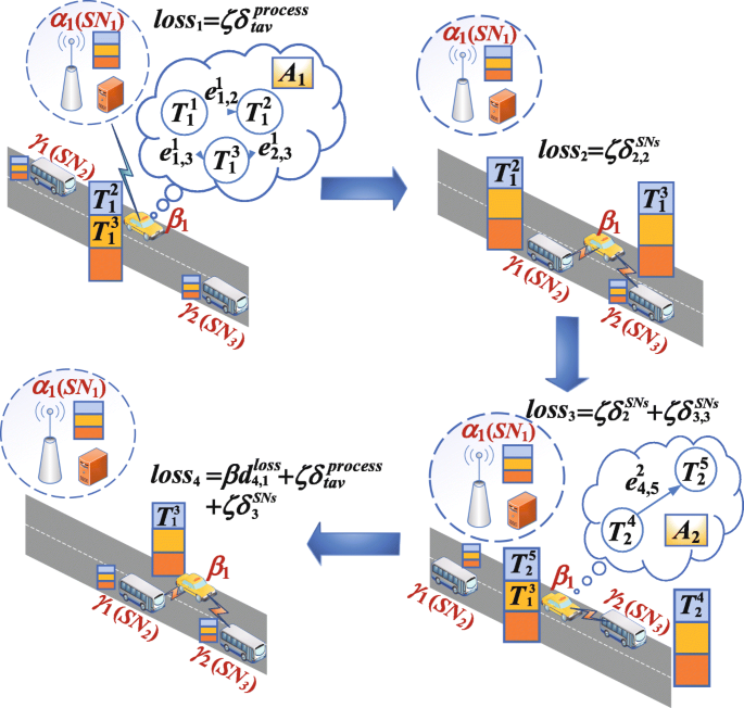
An example analysis of the computation offloading process
-
2)
In the second time slot, TaV transmits task data to γ1. loss2 is energy consumption caused by TaV transmitting task \(\boldsymbol {T}_{1}^{2}\).
-
3)
In the third time slot, TaV generates the second application A2 with the tolerance time of 4 time slots. At this time slot, TaV transmits task data to γ2,loss3 is the weight sum of energy consumption caused by γ1 processing task data and TaV transmitting \(\boldsymbol {T}_{2}^{4}\) to γ2.
-
4)
In the fourth time slot, TaV processes task data locally. At this time slot, the task \(\boldsymbol {T}_{2}^{5}\) is completed, and the task \(\boldsymbol {T}_{1}^{3}\) belonged to A1 has not been processed. So application A1 offloading failed due to that the completion time of A1 is greater than its tolerance time. SeV γ2 processes task data locally, the task \(\boldsymbol {T}_{2}^{4}\) is completed, then all the tasks of A2 have been processed, so A2 are executed successfully. loss4 is the weight sum of total data size of unprocessed task \(d_{4,1}^{loss}\) and the energy consumption caused by TaV processing locally as well as the energy consumption caused by γ2 processing task.

Computational offloading strategy based on deep reinforcement learning
Reinforcement Learning (RL) algorithms have four key elements in model building: agent, environment, action and reward. It is usually modeled as Markov Decision Process (MDP) model.
In the algorithm learning process, the agent observes the current environment and chooses actions according to strategy. After executing the action, the agent observes the reward and transfers to the next environment. RL algorithms imitate the way of human learning. The purpose of RL algorithms is to maximize the total reward by adjusting the strategy appropriately when the agent interacts with the unknown environment.
In this section, we first describe the computation offloading problem by an MDP model to determine the four key elements. Secondly, we introduce Q-learning algorithm. Finally, due to the large dimension of state space in VEC environment, the traditional reinforcement learning optimization method is almost impossible to solve complex computation offloading problem in VEC. Therefore, we adopt SA-DQN to optimize the computation offloading strategy, and describe the computation offloading strategy based on SA-DQN.
MDP model
In order to design the computation offloading strategy based on SA-DQN, we first establish an MDP model. It can fully describe the offloading scheduling model.
MDP model is the basic model of RL algorithms. Since the probability of state transition in real environment is often related to historical state, it is difficult to establish the model. Therefore, the model can be simplified according to Markov property (i.e. the next state in the environment is only related to the current state information, but not to the historical state), so that the next state is only related to the current state and the action taken [34]. Next, we will introduce each key element of MDP.
We define the state space as \({\boldsymbol {S}_{k}} \buildrel \Delta \over = \{{\boldsymbol {\Omega }_{k}},{\boldsymbol {O}_{k}}\} \) in k-th time slot, where \({\boldsymbol {\Omega }_{k}}{=\{x_{k}^{tav},y_{k}^{tav}\}}\) is the two-dimensional coordinates of TaV. Ok represents the distance between TaV and SNs which can be expressed as \({\boldsymbol {O}_{k}} = \{ f(\Phi _{k,1}^{SN}),f(\Phi _{k,2}^{SN}),...,f(\Phi _{k,n + m}^{SN})\} \). If SN is out of communication range, then \(f(\Phi _{k,1}^{SN}) = - 1\), else \(f(\Phi _{k,i}^{SN}) = \Phi _{k,i}^{SN}\). The action space can be described as \({\boldsymbol {A}_{k}} \buildrel \Delta \over = \{ o{l_{k}},\boldsymbol {OS}_{k}^{i},\boldsymbol {OR}_{k}^{i}\} \) in k-th time slot, where olk indicates whether tasks are processed locally by TaV, \(\boldsymbol {OS}_{k}^{i} = \{ os_{k}^{1},os_{k}^{2},...,os_{k}^{n}\} \) indicates whether tasks are offloaded to SeV i and \(\boldsymbol {OR}_{k}^{i} = \{ or_{k}^{1},or_{k}^{2},...,or_{k}^{m}\} \) indicates whether tasks are offloaded to RSU i. The reward can be described as \({r_{k}} \buildrel \Delta \over = 1/los{s_{k}}\) in k-th time slot. The problem of computation offloading for CAV in VEC environment can be described as the following MDP model:
-
Agent:TaV
-
State: Sk
-
Action: Ak
-
Reward: rk
Q-Learning algorithm
In this section, we introduce the traditional RL algorithm called Q-learning. Q-learning is a temporal difference (TD) algorithm based on stochastic process and model-free, and has no state transition probability matrix. The algorithm will select the maximum value for updating the value function, while the action selection does not necessarily follow the action corresponding to the maximum value. It will lead to an optimistic estimation of the value function. Due to this feature, Q-learning belongs to the off-line policy learning method [35].
Q-learning optimizes the value function by four tuple information 〈Sk,Ak,Rk,Sk+1〉, where Sk represents the environmental state in k-th time slot, Ak represents the current action chose, Rk represents the immediate reward, and Sk+1 represents the environmental state of the next time slot after the state transition.
The Q-learning value function is updated as follows:
where α is the learning efficiency, representing the degree of value function updating; r is the immediate reward, representing the reward obtained by transferring to the next state; γ is the discount factor, representing the impact of the subsequent state’s value on the current state; and \({\max _{{A_{k + 1}}}}Q({S_{k + 1}},{A_{k + 1}})\) is the maximum value of next state.
The Equation (17) can be further expressed as
where
In other words, the updating of Q-learning value function can be expressed as the value function’s value plus the product of the difference between target Q-value and estimated Q-value and the learning efficiency. It is also known as TD target.
SA-DQN algorithm
The value function in Q-learning algorithm can be designed simply by a table. But in practice, the state space of computation offloading problem in VEC is large. If we want to establish a value function table, it will lead to serious memory usage and time cost. To solve this problem, known as dimensional disaster, we describe the computation offloading problem as a DRL process, using the function approximation to combine Q-learning with Deep Neural Network (DNN), transform the value function table into Q-network, and adjust the network weight coefficient by algorithm training to fit the value function [36].
Compared with Q-learning, DQN has three main advantages:
-
i)
The Q-network can be expressed as Q(Sk,Ak;θ). θ represents the weights of the neural network, and the Q-network fit value function by updating the parameter θ in each iteration.
-
ii)
In order to improve the learning efficiency and remove the correlation in the subsequent training samples, DQN adopts experience replay technique in the learning process. The sample observed in k-th time slot ek=〈Sk,Ak,Rk,Sk+1〉 is stored into the reply memory D first, and then a sample is randomly chosen from D to train the network. It breaks the correlation among samples and makes them independent.
-
iii)
Two neural networks with the same structure but different weights are used in DQN. One is called the target Q-network, and the other is the estimated Q-network. The estimated Q-network has the latest weights, while the weights of the target Q-network are relatively fixed. The weights of the target Q-network is only updated with the estimated Q-network every ι time slots.
The network used to calculate TD target is called TD-network. If the network parameters used in the value function are the same as those of TD network, it is easy to cause the correlation among samples and make the training unstable. In order to solve this problem, two neural networks are introduced. The weights of the target Q-network can be expressed as \({\bar \theta _{k}}\) and that of estimated Q-network can be expressed as θk, where \({\bar \theta _{k}}{\mathrm { = }}{\theta _{k - \iota }}\), it means that \({\bar \theta _{k}}\) is updated with θk every ι time slots. In DQN algorithm, Equation (17) is transformed into:
In order to minimize the difference between the estimated value and the target value, we define the loss function as follows:
By deriving L(θk) over θk, we obtain the gradient:
Therefore, the updating of value function in DQN is transformed to use gradient descent method to minimize the loss function:
In order to balance the exploration and exploitation of DQN, the Metropolis criterion [37] is used to choose the action, and cooling strategy is described as follows:
where T0 is the initial temperature, k is the amount of current episode, and θ is the cooling coefficient.
The computation offloading strategy based on SA-DQN algorithm is shown in Algorithm 1. In every episode, VEC network needs to be initialized, as shown in Algorithm 2. Then it needs to determine if there is communication interruption and handle it in every time slot, as shown in Algorithm 3. After TaV chooses the offloading decision, the VEC network needs to be updated, as shown in Algorithm 4. If TaV chooses to process tasks locally, the task queue of TaV needs to be updated, as shown in Algorithm 5. If TaV choose to transmit tasks to SNs, the task queue of TaV and SNs also needs to be updated, as shown in Algorithm 6. It needs to determine whether there are applications that offloading failed as it can not complete within its tolerance time in every time slot, as shown in Algorithm 7. The interaction among algorithms is shown in Fig. 5.

The interaction among algorithms


Experimental results and analysis
Parameter settings
All the simulation experiments were conducted on a Win10 64-bit operating system with a Intel(R) Core(TM) i7-4720HQ CPU @ 2.60GHz processor and 8GB RAM. We use TensorFlow 1.15.0 with Python 3.6 to implement SA-DQN algorithm. In the experiment, we consider the real vehicle trajectory data set of two hours in the morning (7.00-9.00) on a circular road in cretey, France [38]. The communication radius of the vehicle is 130 meters. The road conditions include a roundabout with 6 entrances and exits, multiple two lane or three lane roads, one bus road, four lane change points, and 15 traffic lights. In the data set, the trajectory of vehicle with vehicle ID “BusFlowWestEast0.0” is considered as the trajectory of TaV. The trajectory of vehicle with vehicle ID “VehicleFlowWestToEast.0” is considered as the trajectory of the first SeV, and the trajectory of vehicle with vehicle ID “VehicleFlowWestToEast_0.0” is considered as the trajectory of the second SeV. In the center of the TaV’s trajectory, i.e. the two-dimensional coordinate (1250,600), we place an RSU with a coverage radius of 300 meters. β is set to 0.4 and ζ is set to 0.6. There are six CAV’s applications, each application can be divided into three tasks. The length of the time slot is set to 10 ms. The range of data size is distributed uniformly from 1 to 2, and the range of tolerance time is distributed uniformly from 50 to 100 time slots. Table 2 is the detailed setting of simulation parameters. After a number of experiments on parameter adjustment of the RL algorithms to achieve good convergence, parameters setting of RL algorithms is shown in Table 3.
Comparative offloading strategies
In order to verify the effectiveness of our proposed computation offloading strategy, we designed comparative offloading strategies from two perspectives: different RL algorithms and different offloading schemes.
In the first part, we select TD(0) algorithm combined with simulated annealing: Q-learning [39], Sarsa [40] and TD(λ) algorithm [41] with that: Sarsa(λ), Q-learning(λ) as comparative algorithms.
In the second part, we select four schemes for comparison. It is described as follows: Scheme 1 is our proposed strategy; Scheme 2 only considers tasks processed by TaV; Scheme 3 only considers tasks processed by TaV or offloaded to RSU; Scheme 4 only considers tasks processed by TaV or offloaded to cooperative vehicle.
Experimental results
Offloading strategies with different algorithms
Figure 6 shows the average reward of computation offloading strategy based on SA-DQN and comparative algorithms in every 20 episodes. It can be seen that, in the process of optimizing the offloading strategy, SA-DQN continuously interacts with the environment in every episode, updates the weights of neural network, and approaches the optimal value function. With the amount of episodes increasing, the reward increased. Around the 80th episode, the average reward obtained by SA-DQN tends to be optimal and stable, and remained at about 978. Compared with the comparative algorithms, SA-DQN has faster convergence speed. TD(λ) algorithms converged around the 100th round, while TD(0) algorithm converged around the 120th round. It indicates that TD(λ) algorithm converges faster than TD(0) algorithms. The possible reason is that TD(λ) algorithms introduces eligibility trace and adopts multi-step updating strategy. Therefore, it can accelerate the convergence speed. In the experiment, SA-DQN does not encounter the problems of divergence and oscillation, which proves the feasibility computation offloading strategy based on SA-DQN proposed in this paper.

Average reward in every 20 episodes
Figure 7 shows the average total offloading energy consumption of strategy optimized by SA-DQN and comparative algorithms in every 20 episodes. It can be seen that the average offloading total energy consumption of SA-DQN and comparative algorithms is decreasing. Around the 160th episode, the average total offloading energy consumption of each algorithm tends to be optimal and stable. Compared with the comparative algorithms, the average total offloading energy consumption of SA-DQN can be maintained at about 30, reaching a lowest energy consumption level. In the comparative algorithms, the average total offloading energy consumption of Sarsa and Sarsa(λ) algorithms maintained at about 35, while that of Q-learning and Q-learning(λ) algorithms maintained at about 40. This shows that the online learning method can converge to a lower level than the offline learning method in optimizing the average total offloading energy consumption. This is because the online learning method updates the value function by the samples generated by the current strategy. Therefore it can converge faster, but the disadvantage is that it is easy to fall into the local optimal solution.

Average total offloading energy consumption in every 20 episodes
Figure 8 shows the average offloading failure rate of applications optimized by SA-DQN and comparative algorithms in every 20 episodes. It can be seen that with the increase of episodes, the average offloading failure rate of every algorithm decreased. In the 160th episode, except for Q-learning, the average offloading failure rate obtained by other algorithms tends to converge, and the average failure rate of SA-DQN can reach a lower level faster than other algorithms. Compared with the offline learning method, the average offloading failure rate of online learning method was lower than that of offline learning method. This shows that the online learning method can converge to a lower level than the offline learning method in optimizing the average offloading failure rate. This is because the online learning method is a conservative strategy, and it can converge to a lower level faster by following the current strategy.

Average offloading failure rate in every 20 episodes
Offloading strategies with different offloading schemes
Figure 9 shows the average application offloading failure rate of offloading strategies based on different schemes varying from data size. It can be seen that with the increase of data size, the average application offloading failure rate of all strategies increased continuously. The average application offloading failure rate obtained by our proposed strategy reached lower level compared with other strategies when data size is 32. It is because Scheme 1 has various offloading methods, and high offloading flexibility. The average offloading failure rate of Scheme 3 is the closest to that of Scheme 1, because the computing capacity of RSU is higher than that of vehicle. Although it requires certain communication energy consumption to offload to RSU, the completion time of tasks can be greatly reduced, and hence the completion time of application is not easy to exceed its tolerance time, so the penalty of offloading failure decreased. The average application offloading failure rate of Scheme 4 is the highest, because its offloading targets include not only local processing, but also cooperative vehicles, which requires a certain transmission time, and the processing capacity of vehicles is limited, which is not enough to process large amount of data. With the increase of data size, the completion time of application is more likely to exceed its tolerance time, and the penalty for application offloading failure will increase significantly. Therefore, it is obvious that the average application offloading failure rate is rising.

Average offloading failure rate of different strategies with varying data size
Figure 10 shows the average application offloading failure rate of offloading strategies with varying from tolerance time. It can be seen that with the increase of tolerance time, the average application offloading failure rate of all strategies decreased. Compared with other strategies, the proposed strategy reached lower level when tolerance time is 90. This is because when the application tolerance time increases, the application can have more time to offload, and the application completion time is less likely to exceed its tolerance time, and hence the application offloading failure rate decreased. The average offloading failure rate of Scheme 3 is the closest to that of Scheme 1. This is because RSU has strong computing capacity, which can greatly reduce the task completion time. With the increase of the application tolerance time, Scheme 3 can make full use of the computing power of RSU. Therefore, it can be seen that the average application offloading failure rate of Scheme 3 is significantly reduced. Compared with other strategies, the average offloading failure rate of Scheme 2 and Scheme 4 stay at a high level. One possible reason is that both Scheme 2 and Scheme 4 offload tasks to the vehicles with the limited processing capacity. with the increase of application tolerance time, the task offloading with large amount of data size may fail. Thus, the application offloading failure rate is high. On the contrary, both Scheme 1 and Scheme 3 can offload tasks to RSU with stronger computing capacity. Therefore, the number of successful offloading applications increases, and the failure rate of application offloading is lower.

Average offloading failure rate of different strategies with varying tolerance time
Conclusion
In order to solve the problem of computation offloading for CAV’s applications in VEC environment, this paper proposed an computation offloading strategy based on SA-DQN algorithm. In the simulation experiment, the proposed strategy was evaluated based on the real vehicle trajectory. The experimental results show that our proposed computation offloading strategy based on SA-DQN algorithm has good performance, and further indicates that the strategy proposed can effectively reduce the total offloading energy consumption and offloading failure rate of CAV.
In the future work, we will further consider to design collaborative computation offloading strategy in End-Edge-Cloud orchestrated architecture, which can transfer complicated computation tasks to remote cloud for further processing, and it can prompt the flexibility of computation offloading. We will consider more dynamic factors in the VEC environment to make it more suitable for the real world model. In addition, we will take on-board applications in real world into account.
Availability of data and materials
The data set of vehicle trajectory is available on http://vehicular-mobility-trace.github.io/.
References
Wang Y, Liu S, Wu X, Shi W (2018) CAVBench: A Benchmark Suite for Connected and Autonomous Vehicles In: 2018 IEEE/ACM Symposium on Edge Computing (SEC), 30–42. https://doi.org/10.1109/sec.2018.00010.
Organization WH, et al (2018) Global status report on road safety 2018: Summary. World Health Organization, Geneva.
Lin K, Lin B, Chen X, Lu Y, Huang Z, Mo YA (2019) Time-Driven Workflow Scheduling Strategy for Reasoning Tasks of Autonomous Driving in Edge Environment In: 2019 IEEE Intl Conf on Parallel Distributed Processing with Applications, Big Data Cloud Computing, Sustainable Computing Communications, Social Computing Networking (ISPA/BDCloud/SocialCom/SustainCom), 124–131. https://doi.org/10.1109/ispa-bdcloud-sustaincom-socialcom48970.2019.00028.
Wang M, Liang H, Deng R, Zhang R, Shen XS (2013) VANET based online charging strategy for electric vehicles In: 2013 IEEE Global Communications Conference (GLOBECOM), 4804–4809. https://doi.org/10.1109/glocomw.2013.6855711.
Kadav P, Asher ZD (2019) Improving the Range of Electric Vehicles In: 2019 Electric Vehicles International Conference (EV), 1–5. https://doi.org/10.1109/ev.2019.8892929.
Dhirani L, Newe T (2020) 5G security in smart manufacturing. ResearchGate. https://doi.org/10.13140/RG.2.2.27292.72320.
Feng J, Liu Z, Wu C, Ji YAVE (2017) Autonomous Vehicular Edge Computing Framework with ACO-Based Scheduling. IEEE Trans Veh Technol 66(12):10660–10675.
Zhao J, Li Q, Gong Y, Zhang K (2019) Computation Offloading and Resource Allocation For Cloud Assisted Mobile Edge Computing in Vehicular Networks. IEEE Trans Veh Technol 68(8):7944–7956.
Adiththan A, Ramesh S, Samii S (2018) Cloud-assisted control of ground vehicles using adaptive computation offloading techniques In: 2018 Design, Automation Test in Europe Conference Exhibition (DATE), 589–592. https://doi.org/10.23919/date.2018.8342076.
Liu L, Chen C, Pei Q, Maharjan S, Zhang Y (2020) Vehicular Edge Computing and Networking: A Survey. Mob Netw Appl. https://doi.org/10.1007/s11036-020-01624-1.
Wu H, Wolter K, Jiao P, Deng Y, Zhao Y, Xu MEEDTO (2021) An Energy-Efficient Dynamic Task Offloading Algorithm for Blockchain-Enabled IoT-Edge-Cloud Orchestrated Computing. IEEE Internet Things J 8(4):2163–2176.
Wu H (2018) Multi-Objective Decision-Making for Mobile Cloud Offloading: A Survey. IEEE Access 6:3962–3976.
Wu Q, Liu H, Wang R, Fan P, Fan Q, Li Z (2020) Delay-Sensitive Task Offloading in the 802.11p-Based Vehicular Fog Computing Systems. IEEE Internet Things J 7(1):773–785.
Zhang K, Mao Y, Leng S, He Y (2017) ZHANG Y. Mobile-Edge Computing for Vehicular Networks: A Promising Network Paradigm with Predictive Off-Loading. IEEE Veh Technol Mag 12(2):36–44.
Jang Y, Na J, Jeong S, Kang J (2020) Energy-Efficient Task Offloading for Vehicular Edge Computing: Joint Optimization of Offloading and Bit Allocation In: 2020 IEEE 91st Vehicular Technology Conference (VTC2020-Spring), 1–5. https://doi.org/10.1109/vtc2020-spring48590.2020.9128785.
Pu L, Chen X, Mao G, Xie Q, Xu J (2019) Chimera: An Energy-Efficient and Deadline-Aware Hybrid Edge Computing Framework for Vehicular Crowdsensing Applications. IEEE Internet Things J 6(1):84–99.
Wang Y, Wang K, Huang H, Miyazaki T, Guo S (2019) Traffic and Computation Co-Offloading With Reinforcement Learning in Fog Computing for Industrial Applications. IEEE Trans Ind Inform 15(2):976–986.
Khayyat M, Elgendy IA, Muthanna A, Alshahrani AS, Alharbi S, Koucheryavy A (2020) Advanced Deep Learning-Based Computational Offloading for Multilevel Vehicular Edge-Cloud Computing Networks. IEEE Access 8:137052–137062.
Xu X, Zhang X, Liu X, Jiang J, Qi L, Bhuiyan MZA (2020) Adaptive Computation Offloading With Edge for 5G-Envisioned Internet of Connected Vehicles. IEEE Trans Intell Transport Syst:1–10.
Liu Y, Wang S, Zhao Q, Du S, Zhou A, Ma X, et al (2020) Dependency-Aware Task Scheduling in Vehicular Edge Computing. IEEE Internet Things J 7(6):4961–4971.
Guo H, Zhang J, Liu J (2019) FiWi-Enhanced Vehicular Edge Computing Networks: Collaborative Task Offloading. IEEE Veh Technol Mag 14(1):45–53.
Dai P, Hang Z, Liu K, Wu X, Xing H, Yu Z, et al (2020) Multi-Armed Bandit Learning for Computation-Intensive Services in MEC-Empowered Vehicular Networks. IEEE Trans Veh Technol 69(7):7821–7834.
Ke H, Wang J, Deng L, Ge Y, Wang H (2020) Deep Reinforcement Learning-Based Adaptive Computation Offloading for MEC in Heterogeneous Vehicular Networks. IEEE Trans Veh Technol 69(7):7916–7929.
Zhan W, Luo C, Wang J, Wang C, Min G, Duan H, et al (2020) Deep-Reinforcement-Learning-Based Offloading Scheduling for Vehicular Edge Computing. IEEE Internet Things J 7(6):5449–5465.
Dai Y, Xu D, Maharjan S, Zhang Y (2019) Joint Load Balancing and Offloading in Vehicular Edge Computing and Networks. IEEE Internet Things J 6(3):4377–4387.
Lee SS, Lee S (2020) Resource Allocation for Vehicular Fog Computing Using Reinforcement Learning Combined With Heuristic Information. IEEE Internet Things J 7(10):10450–10464.
Dong P, Wang X, Rodrigues J (2019) Deep Reinforcement Learning for Vehicular Edge Computing: An Intelligent Offloading System. ACM Trans Intell Syst Technol 10(6).
Sun Y, Song J, Zhou S, Guo X, Niu Z (2018) Task Replication for Vehicular Edge Computing: A Combinatorial Multi-Armed Bandit Based Approach In: 2018 IEEE Global Communications Conference (GLOBECOM), 1–7. https://doi.org/10.1109/glocom.2018.8647564.
Zeng F, Chen Q, Meng L, Wu J (2020) Volunteer Assisted Collaborative Offloading and Resource Allocation in Vehicular Edge Computing. IEEE Trans Intell Transport Syst:1–11.
Qin Y, Huang D, Zhang X (2012) VehiCloud: Cloud Computing Facilitating Routing in Vehicular Networks In: 2012 IEEE 11th International Conference on Trust, Security and Privacy in Computing and Communications, 1438–1445. https://doi.org/10.1109/trustcom.2012.16.
Luo Q, Li C, Luan TH, Shi W (2020) Collaborative Data Scheduling for Vehicular Edge Computing via Deep Reinforcement Learning. IEEE Internet Things J 7(10):9637–9650.
Wang L, Zhang Q, Li Y, Zhong H, Shi W (2019) MobileEdge: Enhancing On-Board Vehicle Computing Units Using Mobile Edges for CAVs In: 2019 IEEE 25th International Conference on Parallel and Distributed Systems (ICPADS), 470–479. https://doi.org/10.1109/icpads47876.2019.00073.
Mao Y, Zhang J, Song SH, Letaief KB (2016) Power-Delay Tradeoff in Multi-User Mobile-Edge Computing Systems In: 2016 IEEE Global Communications Conference (GLOBECOM), 1–6. https://doi.org/10.1109/glocom.2016.7842160.
Sidford A, Wang M, Wu X, Ye Y (2018) Variance Reduced Value Iteration, Faster Algorithms for Solving Markov Decision Processes. Society for Industrial and Applied Mathematics, USA.
Li J, Xiao Z, Li P (2019) Discrete-Time Multi-Player Games Based on Off-Policy Q-Learning. IEEE Access 7:134647–134659.
Li R, Zhao Z, Sun Q, I C, Yang C, Chen X, et al (2018) Deep Reinforcement Learning for Resource Management in Network Slicing. IEEE Access 6:74429–74441.
Su R, Wu F, Zhao J (2019) Deep reinforcement learning method based on DDPG with simulated annealing for satellite attitude control system In: 2019 Chinese Automation Congress (CAC), 390–395. https://doi.org/10.1109/cac48633.2019.8996860.
Lèbre MA, Le Mouel̈ F, Ménard E (2015) On the Importance of Real Data for Microscopic Urban Vehicular Mobility Trace In: Proceedings of the 14th International Conference on ITS Telecommunications (ITST’2015), 22–26, Copenhagen, Denmark. https://doi.org/10.1109/itst.2015.7377394.
Jiang K, Zhou H, Li D, Liu X, Xu S (2020) A Q-learning based Method for Energy-Efficient Computation Offloading in Mobile Edge Computing In: 2020 29th International Conference on Computer Communications and Networks (ICCCN), 1–7. https://doi.org/10.1109/icccn49398.2020.9209738.
Alfakih T, Hassan MM, Gumaei A, Savaglio C, Fortino G (2020) Task Offloading and Resource Allocation for Mobile Edge Computing by Deep Reinforcement Learning Based on SARSA. IEEE Access 8:54074–54084.
Altahhan A (2020) True Online TD(λ)-Replay An Efficient Model-free Planning with Full Replay In: 2020 International Joint Conference on Neural Networks (IJCNN), 1–7.. IEEE, Glassglow.
Acknowledgements
Both Changhang Lin and Yu Lu are corresponding authors.
Funding
This work is partly supported by the Intelligent Computing and Application Research Team of Concord University College, Fujian Normal University under Grant No.2020TD001, the Natural Science Foundation of China under Grant No.62072108, the Industry and Science guide Foundation of Fujian Province under Grant No.2017H0011, the Natural Science Foundation of Fujian Province under Grant No.2019J01286, and the Young and Middle-aged Teacher Education Foundation of Fujian Province under Grant No.JT180098, Fujian Provincial Key Laboratory of Information Processing and Intelligent Control (Minjiang University) under Grant No.MJUKF-IPIC201907, Open Foundation of Engineering Research Center of Big Data Application in Private Health Medicine, Fujian Province University under Grant No.KF2020001.
Author information
Authors and Affiliations
Contributions
Authors’ contributions
Both Bing Lin and Kai Lin drafted the original manuscript and designed the experiments. Changhang Lin provide ideas and suggestions. Yu Lu provided critical review and helped to draft the manuscript. Both Ziqing Huang and Xinwei Chen designed partial experimental work in the preliminary work and contributed to the revised manuscript. The authors read and approved the final manuscript.
Authors’ information
Bing Lin received the B.S. and M.S degrees in Computer Science from Fuzhou University, Fuzhou, China, in 2010 and 2013, respectively, and the Ph.D. degree in Communication and Information System from Fuzhou University in 2016. He is currently an associate professor with the College of Physics and Energy at Fujian Normal University. Now he is the deputy director of the Department of Energy and Materials, and leads the Intelligent Computing research group. His research interest mainly includes parallel and distributed computing, computational intelligence, and data center resource management.
Kai Lin received the B.S. in Software Engineering from Fujian Agriculture and Forestry University, he is currently pursuing the M.S degree in Fujian Normal University. His main research interests include vehicular edge computing and cloud computing.
Changhang Lin received the B.S. and M.S degrees in Computer technology from Fuzhou University. He is currently an professor of the School of Big Data and Artificial Intelligence, Fujian Polytechnic Normal University. His research interest mainly includes Resource scheduling of cloud computing, Edge computing, Federated learning.
Yu Lu is currently an professor the College of Physics and Energy at Fujian Normal University. His research interest mainly includes Intelligent measurement and control technology in new energy technology.
Ziqing Huang is currently pursuing the B.S. degree in Fujian Normal University. Her main research interests include vehicular edge computing and mobile edge computing.
Xinwei Chen received the B.S., M.S. and Ph.D both in Computer Science and Intelligent Robot System from Nankai University, in 2006,2009 and 2012, and he is with College of Computer and Control Engineering, Minjiang University, Fujian Provincial Key Laboratory of Information Processing and Intelligent Control, Fuzhou, 351008, China. His current research interests include Intelligent Robot System, Embeded System and Computer Vision.
Corresponding authors
Ethics declarations
Competing interests
The authors declare that they have no competing interests.
Additional information
Publisher’s Note
Springer Nature remains neutral with regard to jurisdictional claims in published maps and institutional affiliations.
Rights and permissions
Open Access This article is licensed under a Creative Commons Attribution 4.0 International License, which permits use, sharing, adaptation, distribution and reproduction in any medium or format, as long as you give appropriate credit to the original author(s) and the source, provide a link to the Creative Commons licence, and indicate if changes were made. The images or other third party material in this article are included in the article’s Creative Commons licence, unless indicated otherwise in a credit line to the material. If material is not included in the article’s Creative Commons licence and your intended use is not permitted by statutory regulation or exceeds the permitted use, you will need to obtain permission directly from the copyright holder. To view a copy of this licence, visit http://creativecommons.org/licenses/by/4.0/.
About this article

Cite this article
Lin, B., Lin, K., Lin, C. et al. Computation offloading strategy based on deep reinforcement learning for connected and autonomous vehicle in vehicular edge computing. J Cloud Comp 10, 33 (2021). https://doi.org/10.1186/s13677-021-00246-6
Received:
Accepted:
Published:
DOI: https://doi.org/10.1186/s13677-021-00246-6