
Abstract
This paper investigates the existence of positive periodic solutions for a periodic predator-prey model with fear effect and general functional responses. The general functional responses can cover the Holling types II and III functional response, the Beddington–DeAngelis functional response, the Crowley–Martin functional response, the ratio-dependent type with Michaelis–Menten type functional response, etc. Some new sufficient conditions for the existence of positive periodic solutions of the model are obtained by employing the continuation theorem of coincidence degree theory and some ingenious estimation techniques for the upper and lower bounds of the a priori solutions of the corresponding operator equation. Our results considerably improve and extend some known results.
1 Introduction
The dynamic relationship between predators and prey is very common and essential in ecological environments. Consequently, many scholars have studied different types of predator–prey models based on some practical problems. Many scholars have studied the important dynamic properties of the autonomous and nonautonomous predator–prey models such as stability, permanence, extinction, global attractivity, and the existence of periodic and almost periodic solutions. These studies are valuable in exploring and predicting the relationships and patterns of changes between predators and prey. Periodic phenomena, such as seasonal effects of weather, food supply, mating habits, hunting or harvesting seasons [1], are widespread in ecosystems. In the predator–prey model, a wide variety of functional responses are available reflecting how direct killing may occur. The periodic predator–prey models with different functional responses and practical factors have been studied by many scholars. For example, the ratio-dependent functional responses [2, 3], the Holling type functional responses [4–6], the Beddington–DeAngelis functional responses [4, 7–11], the Crowley–Martin functional responses [12–14] (see also the references therein).
Recently, Tripathi et al. [14] studied the following nonautonomous predator–prey model with Crowley–Martin functional response:
where \(x(t)\) and \(y(t)\) denote the population densities of the prey and predators at time t, respectively. In model (1.1), it is assumed that all parameters are continuous and have positive upper and lower bounds. The function \(a(t)\) denotes the intrinsic rate of prey; \(a(t)/b(t)\) denotes carrying capacity in the absence of predation; \(c(t)\) denotes the capturing rate; \(f(t)\) denotes the conversion rate (the coefficient of conversion from prey to predator); \(d(t)\) denotes the death rate of predators; \(r(t)\) denotes the predator density dependence rate (predator population decreases due to competition among the predators). Predators consume prey with a Crowley–Martin type functional response \((c(t)y(t))/ (\alpha (t)+\beta (t)x(t)+\gamma (t)y(t)+q(t)x(t)y(t))\) and contribute to its growth with rate \((f(t)x(t))/ (\alpha (t)+\beta (t)x(t)+\gamma (t)y(t)+q(t)x(t)y(t))\). The function \(\alpha (t)\) measures the half saturation of prey species; \(\beta (t)\) measures the handling time; \(\gamma (t)\) denotes the coefficient of interference among predators; \(q(t)\) denotes the coefficient of interference among predators at the high density of prey. More detailed biological explanations can be found in [10, 14, 15] and the references therein. Tripathi et al. [14] studied the permanence, extinction, global attractivity, and the existence of periodic and almost periodic solutions of model (1.1) in detail. If \(q(t)\equiv 0\), then the functional response of model (1.1) becomes the Beddington–DeAngelis type, and then model (1.1) was studied in [10, 11]; further if \(r(t)\equiv 0\), then model (1.1) was studied in [4, 7–9]. Moreover, if \(\alpha (t)\equiv 0\) and \(q(t)\equiv 0\), the functional response of model (1.1) becomes the ratio-dependent type, then model (1.1) was studied in [3]; further if \(r(t)\equiv 0\), then model (1.1) was studied in [2].
Many biologists realized that the cost of fear should be incorporated along with direct predation in prey–predator interactions [16]. Experiments by Zenette et al. [17] showed that fear of predators alone led to a 40% reduction in the number of offspring that song sparrow parents could produce. In [18], Wang et al. first formulated and investigated a predator–prey model incorporating the cost of fear (indirect effects) and observed that the cost of fear plays a crucial role in changing the dynamics of predator–prey interactions. Further, some predator–prey models with fear effects and different functional responses and practical factors have been studied by many scholars (see, e.g., [19–23]).
Motivated by the above research works, in this paper, we further consider the following periodic predator–prey model with fear effect and general functional responses:
In model (1.2), the predators follow general functional responses to hunt the prey population, and the function \(G(t, x, y)\) satisfies some assumptions which will be given below. In this paper, we always assume that the functions \(a(t)\), \(b(t)\), \(d(t)\), and \(f(t)\) are continuous, positive, and ω-periodic (\(\omega >0\)); the functions \(k(t)\), \(c(t)\), and \(r(t)\) are continuous, nonnegative, and ω-periodic. In addition, some additional restrictions on the parameter functions will be given in our theorem conditions. Here, the term \(F(k(t),y(t))\leq 1\) denotes the cost of anti-predator defense due to fear; \(k(t)\) reflects the level of fear which drives anti-predator behaviors of the prey [18]. We assume that the function \(F(k,y)\) satisfies the following condition (see [18]):
-
(H)
\(F(k,y)\) is continuous on \(\mathbb{R}_{+}^{2}\) and continuously differentiable with respect to \((k, y)^{T}\in \mathbb{R}_{+}^{2}\); \(F(k, y)>0\), \(F(0,y)=1\), \(F(k,0)=1\) for \(k\geq 0\) and \(y\geq 0\); the partial derivatives \(\frac{\partial F(k,y)}{\partial k}\leq 0\) and \(\frac{\partial F(k,y)}{\partial y}\leq 0\) for \(k\geq 0\) and \(y\geq 0\).
Clearly, the function \(F(k, y)\) can cover the following forms: \(1/(1+ky)\), \(1/(1+ky^{2})\), \(e^{-ky}\), etc.
For convenience, in this paper, we always assume that \(m(t)\), \(\alpha _{1}(t)\), \(\alpha _{3}(t)\), and \(\alpha _{5}(t)\) are continuous, positive, and ω-periodic, \(\alpha _{2}(t)\) and \(\alpha _{4}(t)\) are continuous, nonnegative, and ω-periodic. In addition, we assume that the function \(G(t, x, y)\equiv G_{1}(t, x, y)\) or \(G(t, x, y)\equiv G_{2}(t, x)\), or \(G(t, x, y)\equiv G_{3}(m(t), \frac{x}{y})\), where \(G_{1}(t, x, y)\), \(G_{2}(t, x)\) and \(G_{3}(m(t), \frac{x}{y})\) satisfy some of the given assumptions.
Assume that the function \(G_{1}(t, x, y)\) satisfies the following conditions:
-
(P1)
\(G_{1} (t,x,y)\) is nonnegative and continuous on \(\mathbb{R}\times \mathbb{R}_{+}^{2}\) and continuously differentiable with respect to \((x, y)^{T}\in \mathbb{R}_{+}^{2}\), and ω-periodic in t.
-
(P2)
\(G_{1}(t,x,y)>0\) and \(G_{1}(t,0,y)=0\) for \(t\in \mathbb{R}\), \(x>0\), \(y\geq 0\); for each \((t, y)^{T}\in \mathbb{R}\times \mathbb{R}_{+}\), \(G_{1}(t,x,y)\) is increasing with respect to x on \(\mathbb{R}_{+}\); for each \((t, x)^{T}\in \mathbb{R}\times \mathbb{R}_{+}\), \(G_{1}(t,x,y)\) is nonincreasing with respect to y on \(\mathbb{R}_{+}\).
-
(P3)
There exists a continuous ω-periodic function \(\Theta _{1}(t)>0\) such that \(G_{1}(t,x,0)\leq \Theta _{1}(t)x\) for \(t\in \mathbb{R}\), \(x\in \mathbb{R}_{+}\).
-
(P4)
For each \(x\in (0, +\infty )\), there exists a continuous function \(\widetilde{G_{1}}(t, x)>0\), which is ω-periodic in t, such that \(yG_{1}(t,x,y)\leq \widetilde{G_{1}}(t, x)\) for \(t\in \mathbb{R}\), \(y\geq 0\).
-
(P5)
The partial derivatives \(\frac{\partial G_{1}(t,x,y)}{\partial x}\geq 0\) and \(\frac{\partial G_{1}(t,x,y)}{\partial y}<0\) for \(t\in \mathbb{R}\), \(x>0\), \(y>0\); for each \((t, x)^{T}\in \mathbb{R}\times \mathbb{R}_{+}\), \(\lim_{y\rightarrow \infty}G_{1}(t,x,y)=0\).
It is not difficult to find that \(G_{1}(t, x, y)\) can cover some common forms such as the Beddington–DeAngelis functional response
the Crowley–Martin functional response
and other forms of functional response, such as
Assume that the function \(G_{2}(t, x)\) satisfies the following conditions:
-
(Q1)
\(G_{2} (t,x)\) is nonnegative and continuous on \(\mathbb{R}\times \mathbb{R}_{+}\) and continuously differentiable with respect to \(x \in \mathbb{R}_{+}\), and ω-periodic in t.
-
(Q2)
\(G_{2}(t,x)>0\) and \(G_{2}(t,0)=0\) for \(t\in \mathbb{R}\), \(x>0\); for each \(t\in \mathbb{R}\), \(G_{2}(t,x)\) is increasing with respect to x on \(\mathbb{R}_{+}\).
-
(Q3)
There exists a continuous ω-periodic function \(\Theta _{2}(t)>0\) such that \(G_{2}(t,x)\leq \Theta _{2}(t)x\) for \(t\in \mathbb{R}\), \(x\in \mathbb{R}_{+}\).
-
(Q4)
The partial derivative \(\frac{\partial G_{2}(t,x)}{\partial x}>0\) for \(t\in \mathbb{R}\), \(x>0\).
Clearly, the function \(G_{2}(t,x)\) can cover the classical Holling type II functional response
Note that, for \(x\geq 0\), \(n\in N^{+}\), and \(n\geq 2\),
where
In addition, it is not difficult to verify that the function \(\overline{G_{2}}(t, x)\) satisfies conditions (Q1)–(Q4). Note that, when \(n=2\), the function \(\overline{G_{2}}(t, x)\) becomes the classical Holling type III functional response
Assume that the function \(G_{3}(m, z)\) (\(z=\frac{x}{y}\)) satisfies the following conditions:
-
(H1)
\(G_{3} (m,z)\) is nonnegative and continuous on \(\mathbb{R}_{+}^{2}\) and continuously differentiable with respect to \(z \in \mathbb{R}_{+}\).
-
(H2)
\(G_{3}(m,z)>0\) and \(G_{3}(m,0)=0\) for \(m>0\), \(z>0\); for each \(z>0\), \(G_{3}(m,z)\) is nonincreasing with respect to m on \((0, +\infty )\); for each \(m>0\), \(G_{3}(m,z)\) is increasing with respect to z on \((0, +\infty )\).
-
(H3)
For each \(m>0\), \(\frac{\partial G_{3}(m,z)}{\partial z}>0\) for \(z>0\), and \(\lim_{z\rightarrow \infty}G_{3}(m,z)=\Theta _{3}(m)>0\).
-
(H4)
For each \(m>0\), \(\frac{G_{3}(m,z)}{z}\) is nonincreasing with respect to z on \((0,+\infty )\), and \(\lim_{z\rightarrow 0^{+}}\frac{G_{3}(m,z)}{z}=\Theta _{4}(m)>0\).
It is not difficult to find that \(G_{3}(m(t), \frac{x}{y})\) can cover the ratio-dependent type with Michaelis–Menten functional response
The main purpose of this paper is to study the existence of positive periodic solutions for model (1.2) by using the continuation theorem of coincidence degree theory [24]. The most crucial aspect of using the coincidence theorem is to estimate the upper and lower bounds of the a priori solutions of the corresponding operator equation (see \(L\varphi =\mu N\varphi \), \(\mu \in (0,1)\) in Sect. 2). The existence of positive periodic solutions for the special cases of model (1.2) has attracted the attention of many scholars and has yielded plentiful results (see, e.g., [2–4, 7–11, 14]). For model (1.2), our main results (see Theorems 3.1 and 3.2, Corollary 3.1) extend and improve Theorem 4.2 in Li and She [10], Theorem 3.1 in Li and She [3], Theorem 8 in Tripathi [14]. In addition, we obtain different results compared to some of the known ones (see Theorem 3.5 in Fan et al. [2], Theorems 3.1 and 3.2 in Fan and Kuang [7], Theorems 3.1 and 3.2 in Bohner et al. [4], Theorems 1 and 2 in Fazly and Hesaaraki [9], Theorem 3.1 in Jiang [11], Theorem 9 in Tripathi [14]). It is worth mentioning that the continuation theorem of coincidence degree theory [24] is very effective to study the existence of periodic solutions of predator–prey models (see, e.g., [2, 4–7, 9, 11–14, 25]) and other biological models (see, e.g., [26–28]).
The rest of this paper is organized as follows. In Sect. 2, we first review the continuation theorem of coincidence degree theory [24] and then study the existence of positive periodic solutions of model (1.2). In Sect. 3, we give some applications of our results and compare them with some known results. The last section contains the conclusions and some numerical simulations of this paper.
2 Existence of positive periodic solutions of the model
Let X, Z be normed vector spaces, \(L: \operatorname{Dom} L\subset X \rightarrow Z\) be a linear mapping, \(N: X\rightarrow Z\) be a continuous mapping. The mapping L will be called a Fredholm mapping of index zero if \(\operatorname{dim} \operatorname{Ker} L= \operatorname{codim} \operatorname{Im} L<+\infty \) and ImL is closed in Z. If L is a Fredholm mapping of index zero and there exist continuous projections \(P: X\rightarrow X\) and \(Q: Z\rightarrow Z\) such that \(\operatorname{Im} P= \operatorname{Ker} L\), \(\operatorname{Im} L=\operatorname{Ker} Q=\operatorname{Im}(I-Q)\), it follows that \(L|_{\operatorname{Dom} L \cap \operatorname{Ker} P}:(I-P)X\rightarrow \operatorname{Im} L\) is invertible. We denote the inverse of that map by \(K_{p}\). If Ω is an open bounded subset of X, the mapping N will be called L-compact on Ω̅ if \(QN(\overline{\Omega})\) is bounded and \(K_{p}(I-Q)N: \overline{\Omega}\rightarrow X\) is compact. Since ImQ is isomorphic to KerL, there exists an isomorphism \(J: \operatorname{Im} Q\rightarrow \operatorname{Ker} L\).
Lemma 2.1
([24])
Assume that \(\Omega \subset X\) is an open bounded set. Let L be a Fredholm mapping of index zero, and let N be L-compact on Ω̅. Assume that
-
(i)
\(Lu\neq \mu Nu\), \(\forall u \in \partial \Omega \cap \operatorname{Dom} L\), \(\mu \in (0,1)\);
-
(ii)
\(QNu\neq 0\), \(\forall u \in \partial \Omega \cap \operatorname{Ker} L\);
-
(iii)
\(\operatorname{deg} \{JQN, \Omega \cap \operatorname{Ker} L, 0\}\neq 0\).
Then the operator equation \(Lu=Nu\) has at least one solution in \(\operatorname{Dom} L \cap \overline{\Omega}\).
For any continuous ω-periodic function \(\varrho (t)\) defined on \(\mathbb{R}\), we denote
For convenience, for any \(v, \widetilde{v}\in \mathbb{R}\), we define
The main results of this paper are as follows.
Theorem 2.1
Assume that \(\widehat{c}>0\) and one of the following conditions holds:
-
(A1)
\(G(t, x, y)\equiv G_{1}(t, x, y)\), \(\Pi _{1}:=\frac{1}{\omega}\int _{0}^{\omega}f(t)G_{1} (t,( \frac{a}{b})^{l},0 )\,dt >\widehat{d}\);
-
(A2)
\(G(t, x, y)\equiv G_{2}(t, x)\), \(\Pi _{2}:=\frac{1}{\omega}\int _{0}^{\omega}f(t)G_{2} (t,( \frac{a}{b})^{l} )>\widehat{d}\);
-
(A3)
\(G(t, x, y)\equiv G_{3} (m(t), \frac{x}{y} )\), \(\Pi _{3}:=\Theta _{3}(m^{u})\widehat{f}>\widehat{d}\), \(G_{3} (m^{l},\Upsilon (M_{2}) )< (\frac{d}{f} )^{l}\).
Then model (1.2) has at least one positive ω-periodic solution.
Proof
Assume that \(G(t, x, y)\equiv G_{1}(t, x, y)\) or \(G(t, x, y)\equiv G_{2}(t, x)\), or \(G(t, x, y)\equiv G_{3} (m(t), \frac{x}{y} )\). Let \(x(t)=\exp \{\varphi _{1}(t)\}\) and \(y(t)=\exp \{\varphi _{2}(t)\}\), then model (1.2) can be transformed into
Clearly, it is only necessary to prove that model (2.1) has an ω-periodic solution.
Let
with the norm \(\|\varphi \|=\max_{t\in [0,\omega ]}|\varphi _{1}(t)|+ \max_{t \in [0,\omega ]}|\varphi _{2}(t)|\). Clearly, both X and Z are Banach spaces. Define
where
Then, it has \(\operatorname{Ker} L=\{ \varphi \in X \mid \varphi \in \mathbb{R}^{2}\}\) and \(\operatorname{Im} L=\{\varphi \in Z \mid \int _{0}^{\omega} \varphi (t) \,dt =0 \}\). Clearly, ImL is closed in Z, and \(\operatorname{dim} \operatorname{Ker} L= \operatorname{codim} \operatorname{Im} L=2\). Thus, L is a Fredholm mapping of index zero. Moreover, the generalized inverse (to L) \(K_{P}: \operatorname{Im} L\rightarrow \operatorname{Dom} L\cap \operatorname{Ker} P\) exists and is given by \(K_{P} \varphi =\int _{0}^{t} \varphi (s) \,ds -\frac{1}{\omega}\int _{0}^{ \omega}\int _{0}^{t}\varphi (s)\,ds \,dt \). Then, similar to the proof of Theorem 2.1 in [28], we can obtain that N is L-compact on Ω̅ for any open bounded set \(\Omega \subset X\).
Corresponding to the operator equation \(L\varphi =\mu N\varphi \), \(\mu \in (0,1)\), we have
Assume that \((\varphi _{1}(t),\varphi _{2}(t))^{T} \in X\) is an arbitrary solution of model (2.2) for a certain \(\mu \in (0,1)\). Since \((\varphi _{1}(t),\varphi _{2}(t))^{T} \in X\), there exist \(\xi _{1}\), \(\xi _{2}\), \(\eta _{1}\), \(\eta _{2}\in [0,\omega ]\) such that
Clearly, \(\dot{\varphi}_{1}(\xi _{1})=\dot{\varphi}_{1}(\eta _{1}) = \dot{\varphi}_{2}(\xi _{2})=\dot{\varphi}_{2}(\eta _{2})=0\). Integrating on both sides of (2.2) over the interval \([0,\omega ]\), we have
and
Note that
then we have
From (2.2), (2.3), and condition (H), we have
From (2.3), we have
which implies that
Then, from (2.6), we have
Also, from \(\dot{\varphi}_{1}(\eta _{1}) = 0\), we can easily obtain that
Thus, we have
We consider the following three cases.
Case (i). Condition (A1) holds.
From (2.7), (2.8), and condition (P2), we have
where \(\Delta _{1}(t)=f(t)G_{1}(t,\exp \{M_{1}\},0)\). From (2.5), (2.7), and conditions (P2) and (P4), we have
which implies that
Then, from (2.9), we have
From (2.4) and conditions (P2) and (P3), we have
which implies that
Then, from (2.6), we have
If \(\Pi _{1}>\widehat{d}\), then there exists a sufficiently small constant \(\delta _{1}>0\) such that
Claim (i). If \(\Pi _{1}>\widehat{d}\), then \(\exp \{\varphi _{2}(\eta _{2})\}\geq \delta _{1}\).
If the claim is not true, then
From \(\dot{\varphi}_{1}(\xi _{1})=0\), \(\exp \{\varphi _{2}(\xi _{1})\}\leq \exp \{\varphi _{2}(\eta _{2})\}< \delta _{1}\), conditions (P2) and (P3), we have
Further, from (2.4) and condition (P2), we have
which is a contradiction to (2.10). This proves the claim.
From Claim (i) and (2.9), we can obtain
Now, let us consider the following algebraic equations:
for \((\varphi _{1}, \varphi _{2})^{T}\in \mathbb{R}^{2}\), where \(\mu \in [0,1]\) is a parameter. By using the similar arguments as above, we can show that any solution \((\varphi _{11}^{*}, \varphi _{21}^{*})^{T}\in \mathbb{R}^{2}\) of (2.11) with \(\mu \in [0,1]\) satisfies
where \(\delta ^{*}_{1}>0\) satisfies
Note that \(M_{1}\), \(M_{2}^{(1)}\), \(L_{1}^{(1)}\), \(L_{2}^{(1)}\), \(m_{1}\), \(m_{2}^{(1)}\), \(l_{1}^{(1)}\), and \(l_{2}^{(1)}\) are independent of μ. Define
where
Clearly, \(\Omega ^{(1)}\) satisfies condition (i) in Lemma 2.1. When \(\varphi =(\varphi _{1}, \varphi _{2})^{T}\in \partial \Omega ^{(1)} \cap \operatorname{Ker} L =\partial \Omega ^{(1)} \cap \mathbb{R}^{2}\), then φ is a constant vector in \(\mathbb{R}^{2}\) with \(|\varphi _{1}|+| \varphi _{2}|=U^{(1)}\). Then
where
Here, we have proved that condition (ii) in Lemma 2.1 is satisfied. To compute the Brouwer degree, let us consider the homotopy
where
From (2.12), it follows that \(0\notin \Xi ^{(1)}_{\mu}(\partial \Omega ^{(1)} \cap \mathbb{R}^{2})\) for \(\mu \in [0,1]\). In addition, from conditions (H), (P2), and (P5), one can easily show that \(\Psi ^{(1)} ((\varphi _{1}, \varphi _{2})^{T} )=0\) has a unique solution \((\widetilde{\varphi _{11}^{*}}, \widetilde{\varphi _{21}^{*}})^{T}\) in \(\mathbb{R}^{2}\) if \(\Pi _{1}>\widehat{d}\). Let \(e_{11}=\exp \{\widetilde{\varphi _{11}^{*}}\}>0\), \(e_{21}=\exp \{\widetilde{\varphi _{21}^{*}}\}>0\). From conditions (H) and (P5), we have
A direct calculation produces
Since \(\operatorname{Im} Q = \operatorname{Ker} L\), then we have \(J = I\). Furthermore, by the invariance property of homotopy, we have
By Lemma 2.1, if condition (A1) holds, then model (2.1) admits at least one ω-periodic solution.
Case (ii). Condition (A2) holds.
From (2.7), (2.8), and condition (Q2), we have
where \(\Delta _{2}(t)=f(t)G_{2}(t,\exp \{M_{1}\})\). From (2.4) and condition (Q3), we have
which implies that
Then, from (2.6), we have
From (2.3) and condition (Q2), we have
which implies that
Then, from (2.13), we have
If \(\Pi _{2}>\widehat{d}\), then there exists a sufficiently small constant \(\delta _{2}>0\) such that
Claim (ii). If \(\Pi _{2}>\widehat{d}\), then \(\exp \{\varphi _{2}(\eta _{2})\}\geq \delta _{2}\).
We omit the proof of Claim (ii) here since it is very similar to that of Claim (i).
From Claim (ii) and (2.13), we can obtain
Now, let us consider the following algebraic equations:
for \((\varphi _{1}, \varphi _{2})^{T}\in \mathbb{R}^{2}\), where \(\mu \in [0,1]\) is a parameter. By using similar arguments as above, we can show that any solution \((\varphi _{12}^{*}, \varphi _{22}^{*})^{T}\in \mathbb{R}^{2}\) of (2.14) with \(\mu \in [0,1]\) satisfies
where \(\delta ^{*}_{2}>0\) satisfies
Note that \(M_{1}\), \(M_{2}^{(2)}\), \(L_{1}^{(2)}\), \(L_{2}^{(2)}\), \(m_{1}\), \(m_{2}^{(2)}\), \(l_{1}^{(2)}\), and \(l_{2}^{(2)}\) are independent of μ. Define
where
Clearly, \(\Omega ^{(2)}\) satisfies conditions (i) and (ii) in Lemma 2.1. Let us consider the homotopy
where
where
From (2.15), it follows that \(0\notin \Xi _{\mu}^{(2)}(\partial \Omega ^{(2)} \cap \mathbb{R}^{2})\) for \(\mu \in [0,1]\). In addition, from conditions (H) and (Q2), one can easily show that \(\Psi ^{(2)} ((\varphi _{1}, \varphi _{2})^{T} )=0\) has a unique solution \((\widetilde{\varphi _{12}^{*}}, \widetilde{\varphi _{22}^{*}})^{T}\) in \(\mathbb{R}^{2}\) if \(\Pi _{2}>\widehat{d}\). Let \(e_{12}=\exp \{\widetilde{\varphi _{12}^{*}}\}>0\), \(e_{22}=\exp \{\widetilde{\varphi _{22}^{*}}\}>0\). From conditions (H) and (Q4), we have
Note that \(J=I\), by the invariance property of homotopy, we have
By Lemma 2.1, if condition (A2) holds, then model (2.1) admits at least one ω-periodic solution.
Case (iii). Condition (A3) holds.
From (2.7), (2.8), and conditions (H2) and (H3), we have
From (2.5) and condition (H4), we have
which implies that
Then, from (2.16), we have
From \(\dot{\varphi}_{2}(\eta _{2})=0\), we can obtain
which implies that
Note that
then from condition (H2), we have
Note that
then from \(\dot{\varphi}_{1}(\eta _{1})=0\) and conditions (H), (H2), and (H4), we can obtain
which implies that
Then, from (2.6) and (2.17), we have
If \(\Theta _{3}(m^{u})\widehat{f}>\widehat{d}\), then there exists sufficiently small \(\delta _{3}>0\) such that
Claim (iii). If \(\Theta _{3}(m^{u})\widehat{f}>\widehat{d}\), then \(\exp \{\varphi _{2}(\eta _{2})\}\geq \delta _{3}\).
If the claim is not true, then \(\exp \{\varphi _{2}(\eta _{2})\}<\delta _{3}\). From (2.4) and condition (H2), we have
which is a contradiction to (2.18). This proves the claim.
From Claim (iii) and (2.16), we can obtain
Let \((\varphi _{1}, \varphi _{2})^{T}\in \mathbb{R}^{2}\) satisfy the following algebraic equations:
where \(\mu \in [0,1]\) is a parameter. By using similar arguments as above, we can show that any solution \((\varphi _{13}^{*}, \varphi _{23}^{*})^{T}\in \mathbb{R}^{2}\) of (2.19) with \(\mu \in [0,1]\) satisfies
where \(\delta ^{*}_{3}>0\) satisfies
Note that \(M_{1}\), \(M_{2}^{(3)}\), \(L_{1}^{(3)}\), \(L_{2}^{(3)}\), \(m_{1}\), \(m_{2}^{(3)}\), \(l_{1}^{(3)}\), and \(l_{2}^{(3)}\) are independent of μ. Define
where
Clearly, \(\Omega ^{(3)}\) satisfies conditions (i) and (ii) in Lemma 2.1. To compute the Brouwer degree, let us consider the homotopy
where
From (2.20), it follows that \(0\notin \Xi ^{(3)}_{\mu}(\partial \Omega ^{(3)} \cap \mathbb{R}^{2})\) for \(\mu \in [0,1]\). In addition, from conditions (H), (H2), and (H3), one can easily show that \(\Psi ^{(3)} ((\varphi _{1}, \varphi _{2})^{T} )=0\) has a unique solution \((\widetilde{\varphi _{13}^{*}}, \widetilde{\varphi _{23}^{*}})^{T}\) in \(\mathbb{R}^{2}\) if \(\Pi _{3}>\widehat{d}\). Let \(e_{13}=\exp \{\widetilde{\varphi _{13}^{*}}\}>0\), \(e_{23}=\exp \{\widetilde{\varphi _{23}^{*}}\}>0\). From conditions (H) and (H3), we have
A direct calculation produces
Note that \(J = I\), by the invariance property of homotopy, we have
By Lemma 2.1, if condition (A3) holds, then model (2.1) admits at least one ω-periodic solution. □
3 Some remarks
Our results improve and extend some of the previous results. Some of the remarks below will compare our results with some of the previous results.
If we choose
then model (1.2) becomes the following periodic predator–prey model with Crowley–Martin functional response:
For model (A), an application of our main results is as follows.
Theorem 3.1
Assume that the following condition
holds, then model (A) has at least one positive ω-periodic solution.
A direct corollary of Theorem 3.1 is given below.
Corollary 3.1
Assume that the following condition
holds, then model (A) has at least one positive ω-periodic solution.
Remark 3.1
Recently, Tripathi et al. [14] proved that model (A) has at least one positive ω-periodic solution under the following condition:
Clearly, our condition \((H_{A}^{(2)})\) of Corollary 3.1 is weaker than condition \((H_{A}^{(3)})\). Thus, our Corollary 3.1 improves Theorem 8 in [14].
Remark 3.2
Li and She [10] proved that model (A) has at least one positive ω-periodic solution under the following condition:
Clearly, our condition \((H_{A}^{(2)})\) of Corollary 3.1 is weaker than condition \((H_{A}^{(4)})\). Thus, our Corollary 3.1 improves Theorem 4.2 in [10].
Remark 3.3
Fan and Kuang [7] proved that model (A) has at least one positive ω-periodic solution under the following condition:
In [7], the authors only assumed that the function \(\alpha _{1}(t)\) is nonnegative. If \(\alpha _{1}^{l}>0\), then our condition \((H_{A}^{(2)})\) of Corollary 3.1 is weaker than condition \((H_{A}^{(5)})\). Thus, our Corollary 3.1 extends Theorem 3.1 in [7].
Remark 3.4
For model (A), or some of its special cases, some scholars have obtained some plentiful results of the existence of positive periodic solutions [4, 7–9, 14]. Note that our Theorem 3.1 and Corollary 3.1 do not limit the size of the period ω. Compared with some results in [4, 7, 9, 14] (see Theorem 3.2 in Fan and Kuang [7], Theorem 3.1 in Bohner et al. [4], Theorems 1 and 2 in Fazly and Hesaaraki [9], and Theorem 9 in Tripathi [14]), we obtain different results.
If we choose
then model (1.2) becomes the following periodic ratio-dependent type predator–prey model with Michaelis–Menten type functional response:
For model (B), an application of our main results is as follows.
Theorem 3.2
Assume that the following condition
holds, then model (B) has at least one positive ω-periodic solution.
Remark 3.5
Li and She [3] proved that model (B) has at least one positive ω-periodic solution under the condition
Clearly, our condition \((H_{B}^{(1)})\) of Theorem 3.2 is weaker than condition \((H_{B}^{(2)})\). Thus, our Theorem 3.2 improves Theorem 3.1 in [3].
Remark 3.6
For model (B), if \(r(t)\equiv 0\), then we would like to mention the following two facts.
-
(i)
If model (B) degenerates into the corresponding autonomous system (the case of \(a(t)\equiv a>0\), \(b(t)\equiv b>0\), \(c(t)\equiv c>0\), \(m(t)\equiv m>0\), \(d(t)\equiv d>0\), and \(f(t)\equiv f>0\)), then our condition \((H_{B}^{(2)})\) can be reduced to the sufficient and necessary condition (\(f>d\), \(\frac{c}{a}(1-\frac{d}{f})< m\)) for the existence of the positive equilibrium of model (B) (see [29]).
-
(ii)
Fan, Wang, and Zou [2] proved that model (B) has at least one positive ω-periodic solution under the condition
$$ \bigl(H_{B}^{(3)}\bigr)\quad c^{l}>0,\qquad \widehat{f}>\widehat{d}, \qquad \widehat{a}> \widehat{ \biggl(\frac{c}{m} \biggr)}. $$
As can be seen from (i), we give a different result compared to Theorem 3.5 in [2]. Thus, our Theorem 3.2 extends Theorem 3.5 in [2].
4 Conclusions and numerical simulations
In this paper, the existence of periodic solutions of a class of periodic predator–prey model with fear effect and general functional responses is investigated by means of the continuation theorem of coincidence degree theory [24]. The general functional responses can cover the Holling types II and III functional response, the Beddington–DeAngelis functional response, the Crowley–Martin functional response, the ratio-dependent type with Michaelis–Menten type functional response, etc. The most crucial aspect of using the coincidence theorem is to find a bounded open set Ω that satisfies the conditions of the theorem, which requires estimating the upper and lower bounds on the a priori solution of the corresponding operator equation (\(L\varphi =\mu N \varphi \), \(0<\mu <1\)). This paper mainly obtains three classes of sufficient conditions for the existence of positive periodic solutions of model (1.2). Our main results improve or extend some of the known results (see Remarks 3.1–3.6 in Sect. 3).
At the end of the paper, we present numerical simulations to illustrate our theoretical results. We fix the following parameters: \(a(t)=4+0.5\sin (t)\), \(b(t)=1+0.25\cos (t)\), \(c(t)=1+0.2\cos (t)\), \(d(t)=0.6+0.5\cos (t)\), \(r(t)=3(1+0.5\cos (t))\), \(f(t)=2(1+0.5\cos (t))\).
-
(i)
Let us further choose \(k(t)=3(1+0.5\cos (t))\), \(\alpha _{1}(t)=0.6(1+0.45\sin (t))\), \(\alpha _{2}(t)=0.3+0.2\sin (t)\), \(\alpha _{3}(t)=0.5+0.1\sin (t)\), \(\alpha _{4}(t)=2(1+0.15\sin (t))\). Then we have \(\omega =2\pi \), \(\widehat{c}=1>0\),
$$ \frac{1}{\omega} \int _{0}^{\omega} \frac{f(t)(\frac{a}{b})^{l}}{\alpha _{1}(t)+\alpha _{2}(t)(\frac{a}{b})^{l}}\,dt \approx 4.968889>\widehat{d}=0.6. $$From Theorem 3.1, it follows that model (A) has at least one positive 2π-periodic solution (see Fig. 1).
Figure 1 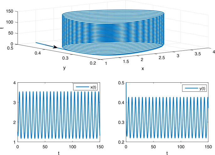
The phase trajectory and solution curves of model (A) with the initial value \((1.5,0.5)^{T}\)
-
(ii)
Let us further choose \(m(t)=0.5+0.1\sin (t)\). Then we have \(\omega =2\pi \), \(\widehat{c}=1>0\),
$$ \widehat{f}=2>\widehat{d}=0.6,\qquad \biggl(\frac{c}{a} \biggr)^{u} \biggl[1- \biggl(\frac{d}{f} \biggr)^{l} \biggr]\approx 0.282176< m^{l}=0.4. $$From Theorem 3.2, it follows that model (B) has at least one positive 2π-periodic solution (see Fig. 2).
Figure 2 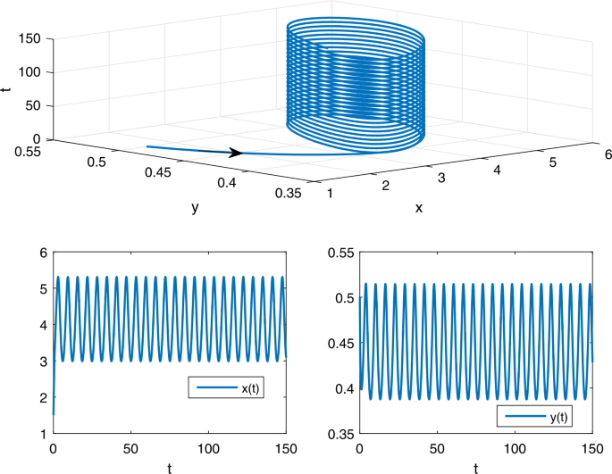
The phase trajectory and solution curves of model (B) with the initial value \((1.5,0.5)^{T}\)


Availability of data and materials
Not applicable.
References
Cushing, J.M.: Periodic time-dependent predator–prey system. SIAM J. Appl. Math. 32, 82–95 (1977)
Fan, M., Wang, Q., Zou, X.: Dynamics of a nonautonomous ratio-dependent predator–prey system. Proc. R. Soc. Edinb., Sect. A 133, 97–118 (2003)
Li, H., She, Z.: Uniqueness of periodic solutions of a nonautonomous density-dependent predator–prey system. J. Math. Anal. Appl. 442, 886–905 (2015)
Bohner, M., Fan, M., Zhang, J.: Existence of periodic solutions in predator–prey and competition dynamic systems. Nonlinear Anal., Real World Appl. 7, 1193–1204 (2006)
Bai, D., Yu, J., Fan, M., Kang, Y.: Dynamics for a non-autonomous predator–prey system with generalist predator. J. Math. Anal. Appl. 485, 123820 (2020)
Zhu, X., Ding, W.: Global stability of periodic solutions of predator–prey system with Holling type III functional response. J. Appl. Anal. Comput. 9, 1606–1615 (2019)
Fan, M., Kuang, Y.: Dynamics of a nonautonomous predator–prey system with the Beddington–DeAngelis functional response. J. Math. Anal. Appl. 295, 15–39 (2004)
Cui, J., Takeuchi, Y.: Permanence, extinction and periodic solution of predator–prey system with Beddington–DeAngelis functional response. J. Math. Anal. Appl. 317, 464–474 (2006)
Fazly, M., Hesaaraki, M.: Periodic solutions for predator–prey systems with Beddington–DeAngelis functional response on time scales. Nonlinear Anal., Real World Appl. 9, 1224–1235 (2008)
Li, H., She, Z.: Dynamics of a non-autonomous density-dependent predator–prey model with Beddington–DeAngelis type. Int. J. Biomath. 9, 1650050 (2016)
Jiang, X., Meng, G., She, Z.: Existence of periodic solutions in a nonautonomous food web with Beddington–DeAngelis functional response. Appl. Math. Lett. 71, 59–66 (2017)
Tripathi, J.P., Jana, D., Vyshnavi Devi, N., Tiwari, V., Abbas, S.: Intraspecific competition of predator for prey with variable rates in protected areas. Nonlinear Dyn. 102, 511–535 (2020)
Cai, M., Yan, S., Du, Z.: Positive periodic solutions of an eco-epidemic model with Crowley–Martin type functional response and disease in the prey. Qual. Theory Dyn. Syst. 19, 56 (2020)
Tripathi, J.P., Bugalia, S., Tiwari, V., Kang, Y.: A predator–prey model with Crowley–Martin functional response: a nonautonomous study. Nat. Resour. Model. 33, e12287 (2020)
Tripathi, J.P., Tyagi, S., Abbas, S.: Global analysis of a delayed density dependent predator–prey model with Crowley–Martin functional response. Commun. Nonlinear Sci. Numer. Simul. 30, 45–69 (2016)
Preisser, E.L., Bolnick, D.I.: The many faces of fear: comparing the pathways and impacts of nonconsumptive predator effects on prey populations. PLoS ONE 3, e2465 (2008)
Zanette, L.Y., White, A.F., Allen, M.C., Clinchy, M.: Perceived predation risk reduces the number of offspring songbirds produce per year. Science 334, 1398–1401 (2011)
Wang, X., Zanette, L., Zou, X.: Modelling the fear effect in predator–prey interactions. J. Math. Biol. 73, 1179–1204 (2016)
Chen, J., He, X., Chen, F.: The influence of fear effect to a discrete-time predator–prey system with predator has other food resource. Mathematics 9, 865 (2021)
Cong, P., Fan, M., Zou, X.: Dynamics of a three-species food chain model with fear effect. Commun. Nonlinear Sci. Numer. Simul. 99, 105809 (2021)
Sk, N., Tiwari, P.K., Pal, S.: A delay nonautonomous model for the impacts of fear and refuge in a three species food chain model with hunting cooperation. Math. Comput. Simul. 192, 136–166 (2022)
Liu, T., Chen, L., Chen, F., Li, Z.: Stability analysis of a Leslie–Gower model with strong Allee effect on prey and fear effect on predator. Int. J. Bifurc. Chaos 32, 2250082 (2022)
Qi, H., Meng, X., Hayat, T., Hobiny, A.: Influence of fear effect on bifurcation dynamics of predator–prey system in a predator-poisoned environment. Qual. Theory Dyn. Syst. 21, 27 (2022)
Gaines, R.E., Mawhin, J.L.: Coincidence Degree and Nonlinear Differential Equations. Springer, Berlin (1977)
Bai, D., Zeng, W., Wu, J., Kang, Y.: Dynamics of a non-autonomous biocontrol model on native consumer, biocontrol agent and their predator. Nonlinear Anal., Real World Appl. 55, 103136 (2020)
Bai, Z., Zhou, Y.: Existence of two periodic solutions for a non-autonomous SIR epidemic model. Appl. Math. Model. 35, 382–391 (2011)
Mandal, P.S., Abbas, S., Banerjee, M.: A comparative study of deterministic and stochastic dynamics for a non-autonomous allelopathic phytoplankton model. Appl. Math. Comput. 238, 300–318 (2014)
Guo, K., Song, K., Ma, W.: Existence of positive periodic solutions of a delayed periodic microcystins degradation model with nonlinear functional responses. Appl. Math. Lett. 131, 108056 (2022)
Beretta, E., Kuang, Y.: Global analysis in some delayed ratio-dependent predator–prey systems. Nonlinear Anal., Theory Methods Appl. 32, 381–408 (1998)
Acknowledgements
The authors would like to thank the reviewers and the editor for their careful reading, helpful comments, and suggestions that greatly improved the paper.
Funding
This paper is supported by Project funded by China Postdoctoral Science Foundation (No. 2022TQ0026), the Fundamental Research Funds for the Central Universities (No. FRF-TP-22-102A1), National Natural Science Foundation of China (No. 12201038 and No. 11971055), and Beijing Natural Science Foundation (No. 1202019).
Author information
Authors and Affiliations
Contributions
All authors jointly worked on the results. All authors read and approved the final version of the manuscript.
Corresponding author
Ethics declarations
Competing interests
The authors declare that they have no competing interests.
Additional information
Publisher’s Note
Springer Nature remains neutral with regard to jurisdictional claims in published maps and institutional affiliations.
Rights and permissions
Open Access This article is licensed under a Creative Commons Attribution 4.0 International License, which permits use, sharing, adaptation, distribution and reproduction in any medium or format, as long as you give appropriate credit to the original author(s) and the source, provide a link to the Creative Commons licence, and indicate if changes were made. The images or other third party material in this article are included in the article’s Creative Commons licence, unless indicated otherwise in a credit line to the material. If material is not included in the article’s Creative Commons licence and your intended use is not permitted by statutory regulation or exceeds the permitted use, you will need to obtain permission directly from the copyright holder. To view a copy of this licence, visit http://creativecommons.org/licenses/by/4.0/.
About this article

Cite this article
Guo, K., Ma, W. Existence of positive periodic solutions for a periodic predator–prey model with fear effect and general functional responses. Adv Cont Discr Mod 2023, 22 (2023). https://doi.org/10.1186/s13662-023-03770-8
Received:
Accepted:
Published:
DOI: https://doi.org/10.1186/s13662-023-03770-8