
Abstract
The impact of Newtonian heating on a time-dependent fractional magnetohydrodynamic (MHD) Maxwell fluid over an unbounded upright plate is investigated. The equations for heat, mass and momentum are established in terms of Caputo (C), Caputo–Fabrizio (CF) and Atangana–Baleanu (ABC) fractional derivatives. The solutions are evaluated by employing Laplace transforms. The change in the momentum profile due to variability in the values of parameters is graphically illustrated for all three C, CF and ABC models. The ABC model has proficiently revealed a memory effect.
1 Introduction
Over the past thirty years, fractional derivatives have fascinated multiple researchers as compared to classical derivatives. Also, fractional derivatives are more credible in mathematical modeling of real-world problems. The methodology of a fractional operator involves regular derivatives and the kernel of a fractional operator with a convolution relation. Initially, Caputo [1] and Riemann–Liouville adopted a power-law kernel to produce a fractional operator. However, this fractional operator faced a few obstructions in real-world applications. Caputo and Fabrizio [2] instead adopted a localized exponential kernel to construct a modern fractional operator. Furthermore, Atangana and Baleanu [3] suggested an advanced fractional operator by using an optimized Mittag–Leffler function, being a nonsingular and nonlocal kernel. This fractional operator counters local and singular kernel restrictions of the preceding fractional operators, keeping certain of their features. Applications of fractional calculus have not only been used in the disciplines of engineering and physical sciences but also in other disciplines, such as ecology, geology, viscoelasticity, economics, probability and statistics and fluid dynamics [4–11].
Among different kinds of rate-type fluids, the Maxwell fluid has gained attention in many research areas. It is a viscoelastic fluid that has properties both of viscosity and elasticity. Maxwell fluids are widely used in polymeric industries due to their lower complexity. The impact of MHD recounts the movement of a conducting flow under the influence of a magnetic field. MHD consequently intensifies conductivity during flow, being a sensation in chemical, mechanical and electrical engineering. Cao et al. [12] analyzed a fractional model of a MHD Maxwell nanofluid over a moving plate. Results for a Maxwell fluid on a vibrating plate utilizing CF derivatives and Laplace transforms were acquired by other investigators [13, 14]. Abro et al. [15] solved the model of a MHD Maxwell fluid for velocity and temperature in a porous medium by using the ABC definition. Bai et al. [16] conducted a thermal analysis in fractional MHD Maxwell flow with viscous dissipation. Asif et al. [17] used the CF definition in order to explore a Maxwell fluid with slip effects.
Normally, thermal convection discussion are connected with distinct physical state, for example, surface heat flux, ramped surface heating and uniform boundary temperature. However, the aforementioned conditions are not applicable for some real-life phenomena. For these phenomena, fluids are placed under Newtonian heating conditions. Newtonian heating expresses that the heat-transfer rate through a sidewall is proportional to the local sidewall temperature. Merkin [18] conducted an introductory study on Newtonian heating. Newtonian heating has several applications, including engine cooling, solar radiations, exploration and extraction processes of petroleum industries, and conjugate heat transport around fins. Nowadays, Newtonian heating has attracted many researchers as a result of its efficient prominence in various engineering systems like radiators. Riaz et al. [19, 20] considered a Maxwell fluid with the contribution of Newtonian heating via fractional operators. Imran et al. [21] employed a CF time derivative to investigate a Maxwell fluid with Newtonian heating on a moving plate. Imran et al. [22] analyzed exact solutions of a rate-type model with Newtonian heating by using Laplace, C and CF time derivatives. Also, they studied the comparison between them. Raza and Asad Ullah [23] used Newtonian heating conditions in a fractional Maxwell fluid and analyzed heat transfer by using C and CF derivatives. Vieru et al. [24] found the solutions for velocity, temperature, and concentration profile for flow under Newtonian heating conditions. Said Mad Zain et al. [25] generalized a fractional Bézier curve with shape parameters. Ghomanjani and Noeiaghdam [26] studied the application of a ball curve for solving fractional differential-algebraic equations.
The basic incentive of this paper was to observe the efficacy of fractional-order derivatives to reveal the memory effect for the Maxwell model under Newtonian heating conditions. The impact of emerging parameters onto momentum, mass and energy solutions are plotted from different graphs accompanied by real justifications. Finally, a comparison has been made among C, CF and ABC fractional models.
2 Mathematical model
Assume a Maxwell fluid upon an upright and unbounded plate under the impact of a magnetic field having strength \(B_{0}\). The plate is perpendicular to the y-axis and parallel to the x-axis. Initially, the fluid and the plate are stationary at a fixed temperature \(\tilde{\Upsilon }_{\infty } \). The local sidewall temperature ϒ̃ and the thermal transfer rate through the bounding wall to the fluid are in proportion to each other. The physical model is shown in Fig. 1 and is given in [19, 20].

Physical model
The governing equations are given by [19, 20]:
Suitable initial and boundary conditions are:
The dimensionless parameters to nondimensionalize the above equations are:
Therefore, the dimensionless momentum, energy and mass equations are:
The required nondimensional initial and boundary conditions are:
3 Preliminaries
3.1 Caputo derivative and its Laplace transform
The Caputo derivative and its Laplace transform are given below:
where \(\Gamma ( \cdot )\) represents the Gamma function.
3.2 Caputo–Fabrizio derivative and its Laplace transform
The Caputo–Fabrizio derivative and its Laplace transform are given below:
where \(N(\gamma )\) is the normalization function or a constant depending on γ. Here, consider \(N(\gamma ) = 1\).
3.3 Atangana–Baleanu derivative and its Laplace transform
The Atangana–Baleanu derivative and its Laplace transform are given below:
where \(AB(\gamma )\) represents the normalization function. Here, \(AB(\gamma ) = 1\).
5 Solutions for concentration profile
The concentration fields for integer-order, C and CF time-fractional derivatives have been already calculated by Riaz et al. [20].
6 Solutions for velocity profile
6.1 Integer-order solution
Theorem 1
Let \(\mathcal{L}\) be the Laplace operator, applying this operator to Eq. (4) along with initial and boundary conditions, the exact solution of velocity is given in Eq. (19).
Proof
Applying the Laplace transform to Eq. (4), we obtain:
After some simplifications, we obtain:
Equation (15) is a 2nd-order nonhomogeneous linear equation.
The standard solution of Eq. (15) is
where \(\bar{W}_{1} ( \zeta ,q )\) and \(\bar{W}_{2} ( \zeta ,q )\) are the complementary and particular solutions, respectively.
Here, \(a_{1} = \frac{\Pr - ( 1 + \lambda M )}{\lambda } \), \(a_{2} = \frac{M}{\lambda } \) and \(b_{1} = \frac{Sc - ( 1 + \lambda M )}{\lambda } \).
Putting Eqs. (17) and (18) into Eq. (16), we obtain:
After applying initial and boundary conditions to the above equation, we obtain the Laplace solution for velocity:
where \(a_{3} = \frac{1 + \lambda M}{2\lambda } \), \(a_{4} = \sqrt{\frac{ ( 1 + \lambda M )^{2} - 4\lambda M}{4\lambda ^{2}}}\), \(A_{1} = \frac{a_{1}}{2} - z\), \(A_{2} = \frac{a_{1}}{2} + z\), \(A_{3} = a_{1}^{2} - 4z^{2}\), \(A_{4} = 2z^{2} - a{}_{1}z\), \(A_{5} = 2z^{2} + a{}_{1}z\), \(z = \sqrt{\frac{a_{1}^{2} - 4a_{2}}{4}}\), \(B_{1} = \frac{b_{1}}{2} - z_{1}\), \(B_{2} = \frac{b_{1}}{2} + z_{1}\), \(B_{3} = z_{1}(b_{1} - 2z_{1})^{2}\), \(B_{4} = z_{1}(b_{1} + 2z_{1})^{2}\), \(B_{5} = b_{1}^{2} - 4z_{1}^{2}\) and \(z_{1} = \sqrt{\frac{b_{1}^{2} - 4a_{2}}{4}}\). □
6.2 Caputo fractional derivative
Theorem 2
Let \({}^{C}D_{t}^{\gamma } i(\zeta ,t)\) be the Caputo fractional derivative and L be the Laplace operator, applying these operators to Eq. (4) along with initial and boundary conditions, the exact solution of velocity is given in Eq. (26).
Proof
Applying the Caputo time derivative Eq. (7) to the nondimensional velocity Eq. (4) and taking the Laplace transform, we obtain:
The general solution of the nonhomogeneous linear equation, Eq. (22), is:
Here,
and
Substituting Eq. (24) and Eq. (25) into Eq. (23) and applying initial and boundary conditions, the Laplace solution of Eq. (23) is
where \(m_{1} = q + M\), \(p = \lambda ( q + M ) - \Pr \) and \(s = \lambda ( q + M ) - Sc\). □
6.3 Caputo–Fabrizio fractional derivative
Theorem 3
Let \({}^{CF}D_{t}^{\gamma } i(\zeta ,t)\) be the Caputo–Fabrizio fractional derivative and L be the Laplace operator, applying these operators to Eq. (4) along with initial and boundary conditions, the exact solution of velocity is given in Eq. (33).
Proof
Applying the Caputo–Fabrizio time derivative Eq. (9) and then its Laplace transform Eq. (10) to Eq. (4), we obtain:
After some calculations we obtain a second-order nonhomogeneous linear equation:
The solution of Eq. (29) is
where
and
Inserting the values of Eq. (31) and Eq. (32) into Eq. (30) and applying initial and boundary conditions, we have:
where \(m_{1} = q + M\), \(l = 1 - \gamma \), \(d = 1 - \gamma + \lambda \), \(p_{2} = m_{1}d - \Pr \) and \(s_{2} = m_{1}d - Sc\). □
6.4 Atangana–Baleanu fractional derivative
Theorem 4
Let \({}^{ABC}D_{t}^{\gamma } i(\zeta ,t)\) be the Atangana–Baleanu fractional derivative and L be the Laplace operator, applying these operators to Eq. (4) along with initial and boundary conditions, the exact solution of velocity is given in Eq. (40).
Proof
Applying the Atangana–Baleanu time derivative Eq. (11) and then its Laplace transform Eq. (12) to Eq. (4), we obtain:
Equation (36) is a 2nd-order nonhomogeneous linear equation. So, its exact solution is:
Here,
and
Putting values of the solution of \(\bar{W}_{1} ( \zeta ,q )\) and \(\bar{W}_{2} ( \zeta ,q )\) into Eq. (37) and after some simplifications, we obtain:
where \(m_{1} = q + M\), \(l = 1 - \gamma \), \(d = 1 - \gamma + \lambda \), \(p_{3} = m_{1}d - \Pr \) and \(s_{3} = m_{1}d - Sc\). □
Stehfest’s formula [22] is one of the simplest algorithms we use to determine the inverse Laplace transform:
where \(N_{1}\) is a natural number, \(\operatorname{Re} (\cdot)\) and i are the real part and the imaginary unit, respectively [22].
7 Limiting case
7.1 Case 1
By ignoring the concentration profile, we recover the results presented in Riaz and Iftikhar [19].
7.2 Case 2
By removing the magnetic field in Eq. (4), we obtain the results presented in Riaz et al. [20].
7.3 Case 3
By eliminating the concentration and magnetic field simultaneously we obtain the results shown in Raza and Asad Ullah [23].
8 Results and discussion
In this article, the effects of Newtonian heating on MHD Maxwell flow over a vertical plate are studied. The C, CF and ABC derivatives are interpolated to form three particular fractional models for flow, energy and mass equations. Fractional derivatives and Laplace transforms are applied to examine the solutions for nondimensional fractional models. Limiting cases of the fractional models are discussed. Several graphs are presented to illustrate the physical effects of parameters γ, λ, Sc, Pr, Gr, Gm and M on velocity.
-
1.
Effect of γ: Fig. 2 shows that the fluid velocity increases when the fractional parameter γ increases, as time varies. The rate of change increases, and the velocity profile increases. All curves, Caputo, Caputo–Fabrizio and Atangana–Baleanu, converge as y tends to infinity. For both large and small time and among all three MHD fractional Maxwell models, the fluid velocity is maximum for the Atangana–Baleanu case as it has a nonsingular and nonlocal kernel. For the Caputo fractional model, the fluid velocity is minimum, while for the Caputo–Fabrizio model, the fluid velocity is moderate among all three models because it has a nonsingular kernel and a maximum for the ABC model. The fractional-order derivative converts into a classical model as \(\alpha \rightarrow 1\).
Figure 2 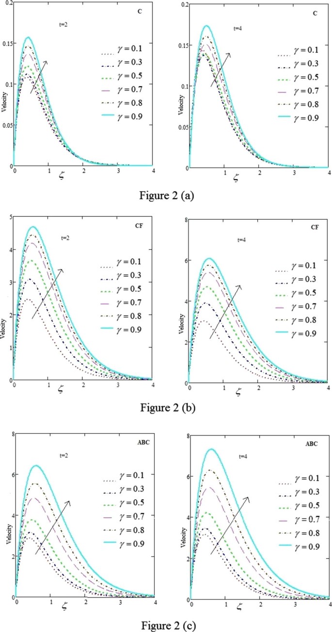
(a, b, c). Velocity curves belonging to C, CF and ABC for various values of γ, where \(M = 4\), \(\Pr = 6\), \(Sc = 8\), \(Gr = 6\), \(Gm = 8\) and \(\lambda = 0.2\)
-
2.
Effect of M: Fig. 3 reveals the deviation in velocity distribution under the effect of a magnetic field. The magnetic field causes a frictional force (Lorentz force) due to which the fluid velocity decreases. For different values of M, an increase in the Lorentz force effectively decreases flow-accelerating forces, and as a result, the velocity is decelerated. The fluid velocity is maximum, moderate and minimum for Atangana–Baleanu, Caputo–Fabrizio and Caputo models, respectively
Figure 3 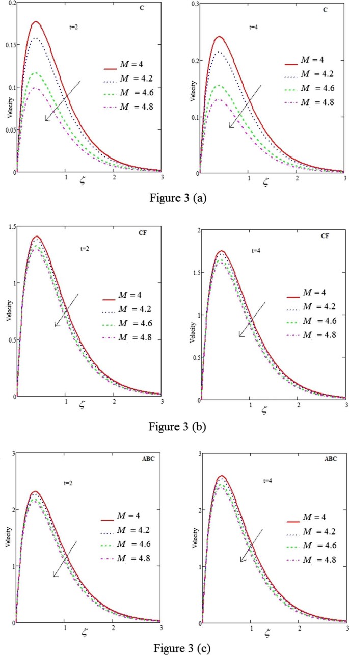
(a, b, c). Velocity curves belonging to C, CF and ABC for various values of M, where \(\gamma = 0.1\), \(\Pr = 6\), \(Sc = 8\), \(Gr = 6\), \(Gm = 8\) and \(\lambda = 0.2\)
-
3.
Effect of λ: Fig. 4 shows that as λ increases, the velocity profile decreases. The velocity function has also been determined for variable time. Relaxation time enhances the backward flow and reduces the velocity. Also, when λ rises, the thickness of the momentum boundary layer minimizes, which leads to a downshift of the flow. Since the increment in relaxation time suggests that fluid will acquire additional time to relax, it affirms a decrease in velocity.
Figure 4 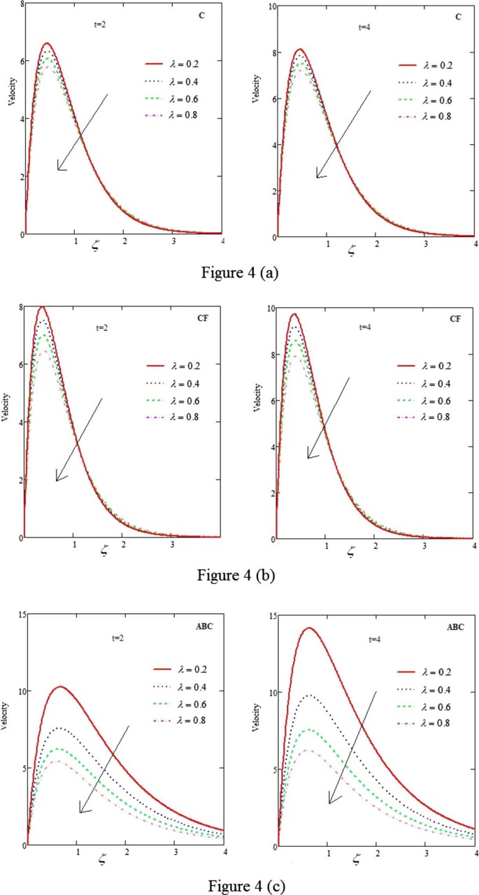
(a, b, c). Velocity curves belonging to C, CF and ABC for various values of λ, where \(\gamma = 0.1\), \(\Pr = 6\), \(Sc = 8\), \(Gr = 6\), \(Gm = 8\) and \(M = 4\)
-
4.
Effect of Sc: The fluid velocity decreases when Sc increases, as shown in Fig. 5. As the Maxwell fractional model concerns the effect of a magnetic field, this causes a decrease in molecular or mass diffusivity and hence velocity decreases. Moreover, Sc is also inversely proportional to the molecular diffusivity due to which the fluid velocity decreases. Among all three fractional solutions, the velocity profile is significant for the Atangana–Baleanu model.
Figure 5 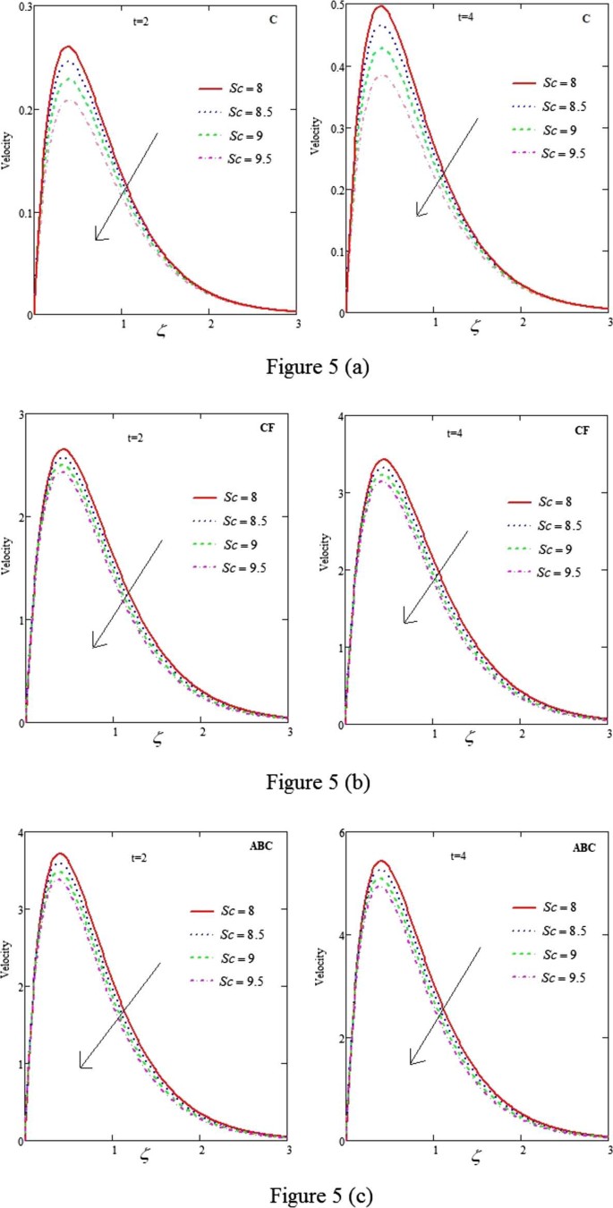
(a, b, c). Velocity curves belonging to C, CF and ABC for various values of Sc, where \(\gamma = 0.1\), \(\Pr = 6\), \(\lambda = 0.2\), \(Gr = 6\), \(Gm = 8\) and \(M = 4\)
-
5.
Effect of Gm: Fig. 6 shows that the fluid velocity increases with increasing Gm. Physically, the increment in buoyancy forces reduces the viscous force that leads to a further increase in the velocity field with higher values of Gm. Velocity curves show maximum behavior for the ABC model as compared to the other two models.
Figure 6 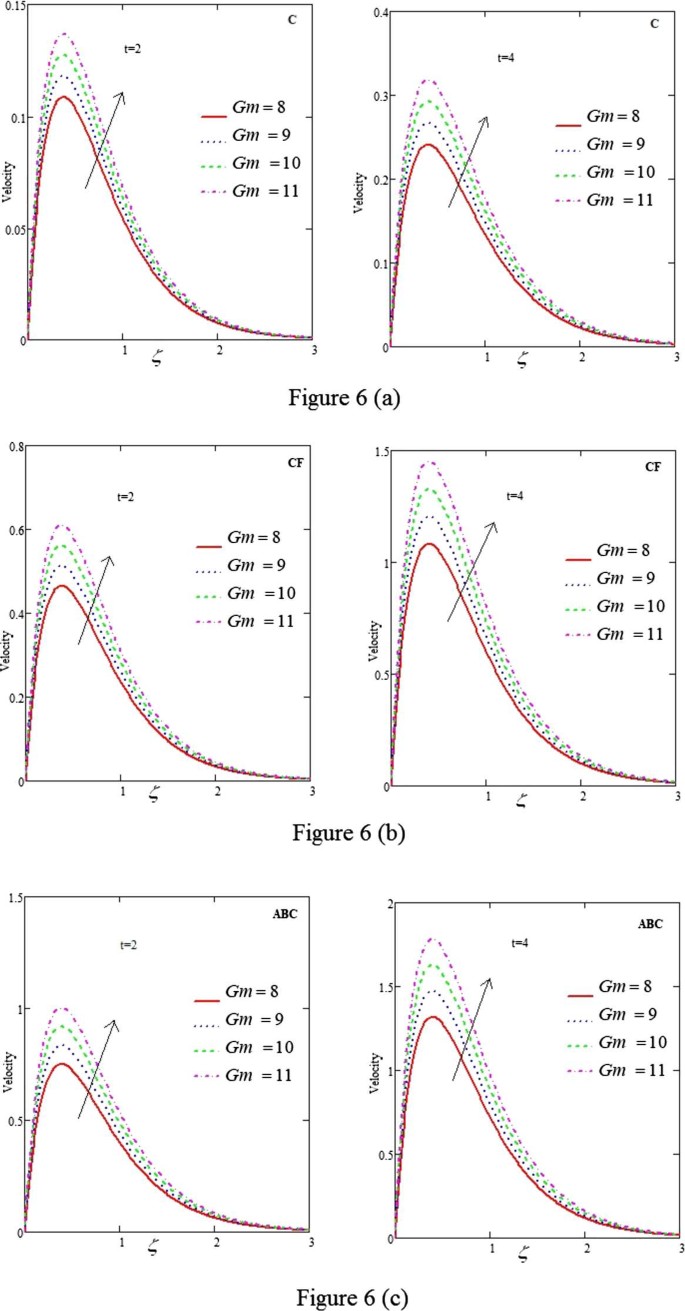
(a, b, c). Velocity curves belonging to C, CF and ABC for various values of Gm, where \(\gamma = 0.1\), \(\Pr = 6\), \(\lambda = 0.2\), \(Gr = 6\), \(Sc = 8\) and \(M = 4\)
-
6.
Effect of Gr: Fig. 7 describes the variability of the momentum profile with increasing values of Grashof number. Physically, large values of Gr correspond to a significant buoyancy force as it is related to strong convection currents. For increasing Gr, all buoyancy forces dominate frictional forces and hence the momentum profile is amplified.
Figure 7 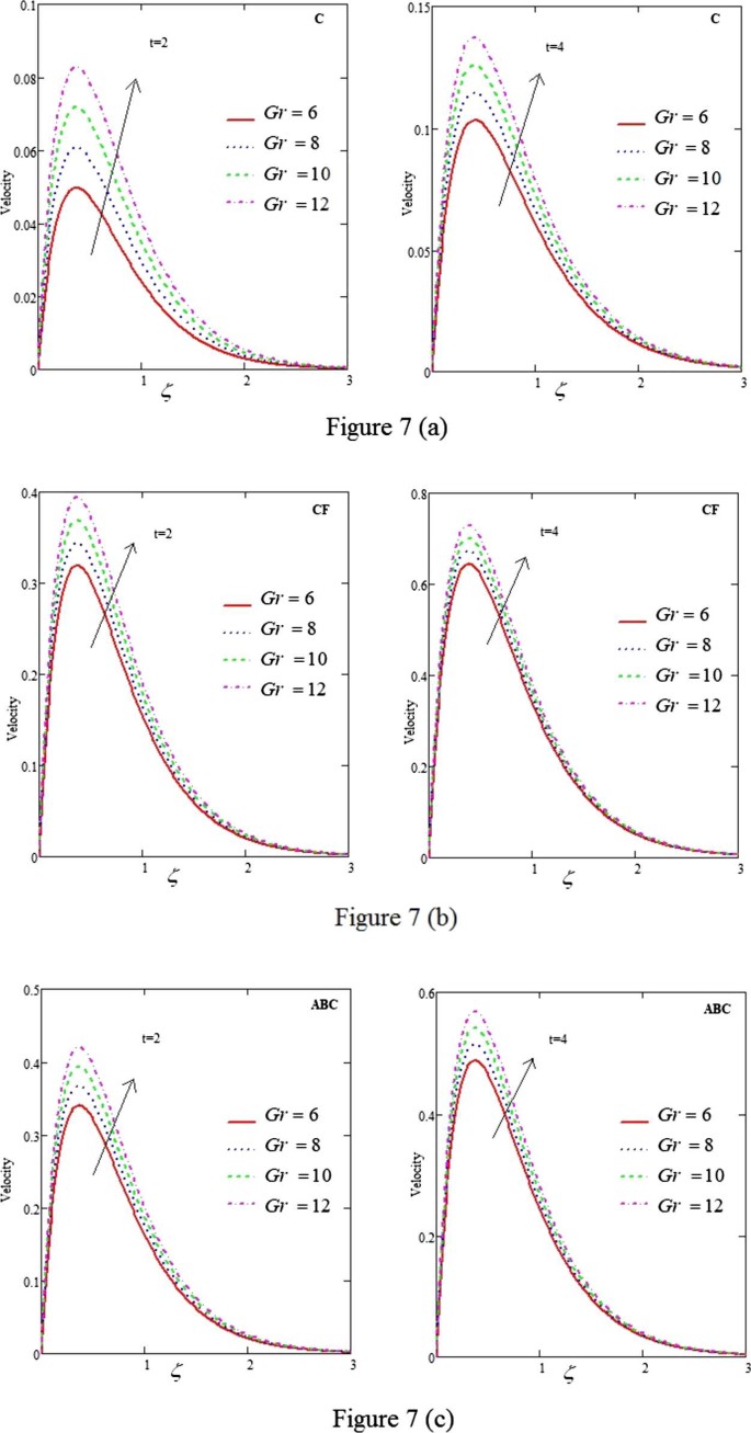
(a, b, c). Velocity curves belonging to C, CF and ABC for various values of Gr, where \(\gamma = 0.1\), \(\Pr = 6\), \(\lambda = 0.2\), \(Sc = 8\), \(Gm = 8\) and \(M = 4\)
-
7.
Effect of Pr: Fig. 8 illustrates the effects of Pr on the flow. It is noted that the flow declines as Pr increases. Clearly, as Pr increases, thermal diffusivity decreases. This causes an increase in viscosity, which results in a decrease in velocity. Moreover, the velocity profile of the MHD Maxwell fractional model is minimum for the Caputo case and maximum for the Atangana–Baleanu case.
Figure 8 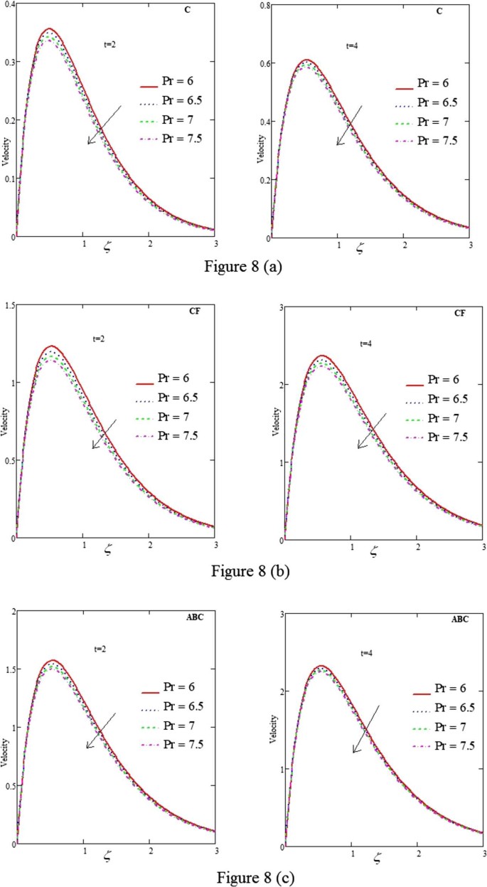
(a, b, c). Velocity curves belonging to C, CF and ABC for various values of Pr, where \(\gamma = 0.1\), \(Gr = 6\), \(\lambda = 0.2\), \(Sc = 8\), \(Gm = 8\) and \(M = 4\)
-
8.
Comparison among C, CF and ABC: Fig. 9 shows a comparison among the three fractional models. Clearly, velocity curves for ABC show a significant change for different values of the fractional parameter.
Figure 9 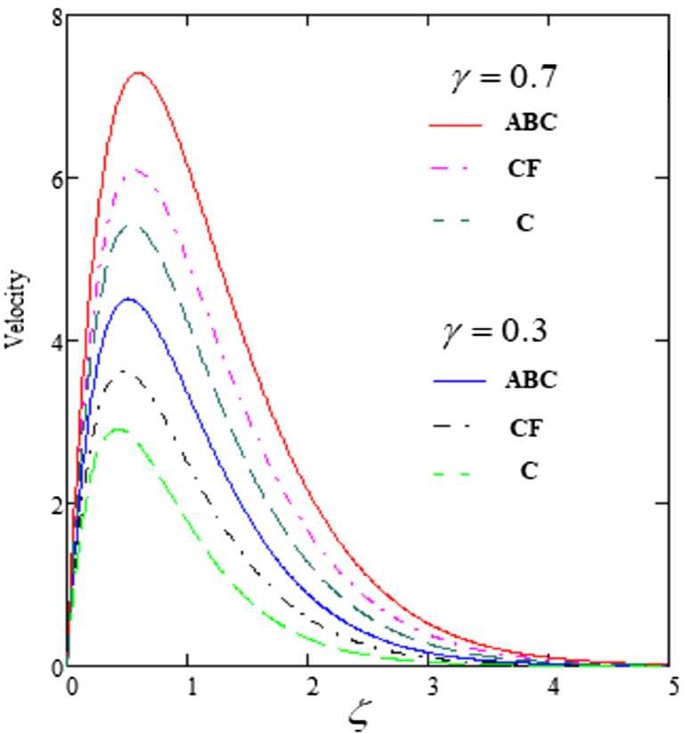
Velocity curves for C, CF and ABC for various values of γ
-
9.
Velocity profile without concentration: Fig. 10 presents the velocity curves for C, CF and ABC without concentration. It is observed that as the fractional parameter tends to 1 the fractional model approaches to an integer-order model [21].
Figure 10 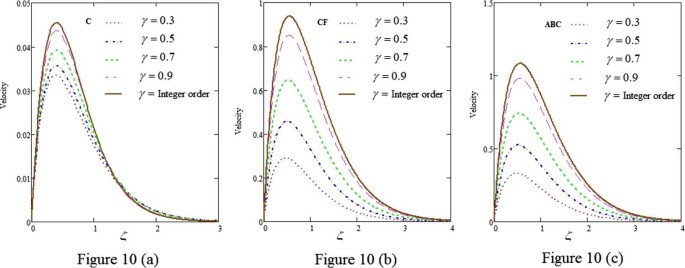
(a, b, c). Velocity curves for C, CF and ABC for various values of γ approaching to integer order


9 Conclusions
This article studies a time-dependent, Maxwell MHD fluid on an unbounded upright plate with Newtonian heating. The C, CF and ABC operators are used to construct a flow-directing equation for a rate-type fluid. Solutions of the model equations are presented from Laplace transforms. Several graphs are presented to illustrate the impact of various parameters on the solutions. Significant findings of this study are noted as follows:
-
1.
The velocity of the fluid increases with increasing fractional parameter for the Caputo, Caputo–Fabrizio and Atangana Baleanu models.
-
2.
The flow profile is maximum for the ABC model as compared to the C and CF models.
-
3.
As the magnetic field increases for variable time, the fluid velocity decreases for local, nonlocal and nonsingular kernels.
-
4.
An increment in the Maxwell parameter λ causes a decrease in the fluid velocity for all fractional models.
-
5.
The fluid velocity declines as the values of Pr and Sc increase, whereas, the fluid velocity exhibits a reverse profile for higher values of Gr and Gm.
Availability of data and materials
Not applicable.
Abbreviations
- W̃ :
-
Fluid velocity
- ϒ̃:
-
Fluid temperature
- Λ̃:
-
Fluid concentration
- \(\tilde{\Upsilon }_{\infty } \) :
-
Temperature of fluid far from the plate
- \(\tilde{\Upsilon }_{w}\) :
-
Temperature of fluid at the plate
- \(\tilde{\Lambda }_{\infty } \) :
-
Concentration of fluid far from the plate
- \(\tilde{\Lambda }_{w}\) :
-
Concentration level on the plate
- g :
-
Gravitational acceleration
- k :
-
Thermal conductivity of the fluid
- h :
-
Coefficient of heat transfer
- ρ :
-
Fluid density
- \(C_{p}\) :
-
Specific heat at constant temperature
- \(\beta _{\tilde{\Upsilon }} \) :
-
Volumetric coefficient of thermal expansion
- \(\beta _{\tilde{\Lambda }} \) :
-
Volumetric coefficient of mass expansion
- Pr:
-
Prandtl number
- Sc :
-
Schmidt number
- Gr :
-
Thermal Grashof number
- Gm :
-
Mass Grashof number
- \(B_{o}\) :
-
Magnitude of applied magnetic field
- M :
-
Hartmann number
- \(D_{m}\) :
-
Mass diffusivity
- λ :
-
Maxwell parameter
- υ :
-
Kinematic viscosity
- μ :
-
Dynamic viscosity
- q :
-
Laplace parameter
References
Podlubny, I.: Fractional Differential Equations: An Introduction to Fractional Derivatives, Fractional Differential Equations, to Methods of Their Solution and Some of Their Applications, vol. 198. Elsevier, Amsterdam (1998)
Caputo, M., Fabrizio, M.: A new definition of fractional derivative without singular kernel. Prog. Fract. Differ. Appl. 1, 1–13 (2015)
Atangana, A., Baleanu, D.: New fractional derivatives with nonlocal and non-singular kernel: theory and application to heat transfer model. Therm. Sci. 2, 763–769 (2016)
Saeed, S.T., Riaz, M.B., Baleanu, D., Abro, K.A.: A mathematical study of natural convection flow through a channel with non-singular kernels: an application to transport phenomena. Alex. Eng. J. 59, 2269–2281 (2020)
Riaz, M.B., Saeed, S.T., Baleanu, D.: Role of magnetic field on the dynamical analysis of second grade fluid: an optimal solution subject to non-integer differentiable operators. J. Appl. Comput. Mech. 7, 54–68 (2021)
Atangana, A.: On the new fractional derivative and application to nonlinear Fisher’s reaction–diffusion equation. Appl. Math. Comput. 273, 948–956 (2016)
Tarasova, V.V., Tarasov, V.E.: Economic interpretation of fractional derivatives. Prog. Fract. Differ. Appl. 3, 1–7 (2017)
Yang, X.J., Machado, J.A.T.: A new fractional operator of variable order: application in the description of anomalous diffusion. Physica A 481, 276–283 (2017)
Zhuravkov, M.A., Romanova, N.S.: Review of methods and approaches for mechanical problem solutions based on fractional calculus. Math. Mech. Solids 21, 595–620 (2016)
Imran, M.A., Aleem, M., Riaz, M.B., Ali, R., Khan, I.: A comprehensive report on convective flow of fractional (ABC) and (CF) MHD viscous fluid subject to generalized boundary conditions. Chaos Solitons Fractals 118, 274–289 (2019)
Du, M., Wang, Z., Hu, H.: Measuring memory with the order of fractional derivative. Sci. Rep. 3, 3431 (2013)
Cao, Z., Zhao, J., Wang, Z., Liu, F., Zheng, L.: MHD flow and heat transfer of fractional Maxwell viscoelastic nanofluid over a moving plate. J. Mol. Liq. 222, 1121–1127 (2016)
Khan, I., Shah, N.A., Mahsud, Y., Vieru, D.: Heat transfer analysis in a Maxwell fluid over an oscillating vertical plate using fractional Caputo–Fabrizio derivatives. Eur. Phys. J. Plus 132, 194 (2017)
Tahir, M., Imran, M.A., Raza, N., Abdullah, M., Aleem, M.: Wall slip and non-integer order derivative effects on the heat transfer flow of Maxwell fluid over an oscillating vertical plate with new definition of fractional Caputo–Fabrizio derivatives. Results Phys. 7, 1887–1898 (2017)
Abro, K.A., Khan, I., Tassaddiq, A.: Application of Atangana–Baleanu fractional derivative to convection flow of MHD Maxwell fluid in a porous medium over a vertical plate. Math. Model. Nat. Phenom. 13, 1 (2018)
Bai, Y., Jiang, Y., Liu, F., Zhang, Y.: Numerical analysis of fractional MHD Maxwell fluid with the effects of convection heat transfer condition and viscous dissipation. AIP Adv. 7, 125309 (2017)
Asif, N.A., Hammouch, Z., Riaz, M.B., Bulut, H.: Analytical solution of a Maxwell fluid with slip effects in view of the Caputo–Fabrizio derivative. Eur. Phys. J. Plus 133, 272 (2018)
Merkin, J.H.: Natural-convection boundary-layer flow on a vertical surface with Newtonian heating. Int. J. Heat Fluid Flow 15, 392–398 (1994)
Riaz, M.B., Iftikhar, N.: A comparative study of heat transfer analysis of MHD Maxwell fluid in view of local and nonlocal differential operators. Chaos Solitons Fractals 132, 109556 (2020)
Riaz, M.B., Atangana, A., Iftikhar, N.: Heat and mass transfer in Maxwell fluid in view of local and non-local differential operators. J. Therm. Anal. Calorim. 143, 4313–4329 (2021)
Imran, M.A., Riaz, M.B., Shah, N.A., Zafar, A.A.: Boundary layer flow of MHD generalized Maxwell fluid over an exponentially accelerated infinite vertical surface with slip and Newtonian heating at the boundary. Results Phys. 8, 1061–1067 (2018)
Asjad, M.I., Shah, N.A., Aleem, M., Khan, I.: Heat transfer analysis of fractional second-grade fluid subject to Newtonian heating with Caputo and Caputo–Fabrizio fractional derivatives: a comparison. Eur. Phys. J. Plus 132, 340 (2017)
Raza, N., Ullah, M.A.: A comparative study of heat transfer analysis of fractional Maxwell fluid by using Caputo and Caputo–Fabrizio derivatives. Can. J. Phys. 98, 89–101 (2019)
Vieru, D., Fetecau, C., Fetecau, C.: Time-fractional free convection flow near a vertical plate with Newtonian heating and mass diffusion. Therm. Sci. 19, 85–98 (2015)
Said Mad Zain, S.A.A.A., Misro, M.Y., Miura, K.T.: Generalized fractional Bézier curve with shape parameters. Mathematics 9, 2141 (2021)
Ghomanjani, F., Noeiaghdam, S.: Application of Said Ball curve for solving fractional differential-algebraic equations. Mathematics 9, 1926 (2021)
Acknowledgements
This Research was supported by Taif University Researchers Supporting Project Number (TURSP-2020/96), Taif University, Taif, Saudi Arabia. The authors are also grateful to the anonymous referees for their valuable suggestions that significantly improved this manuscript.
Funding
No external funding is available for this research.
Author information
Authors and Affiliations
Contributions
All the authors contributed equally to this work. All the authors read and approved the final manuscript.
Corresponding author
Ethics declarations
Competing interests
The authors declare that they have no competing interests.
Rights and permissions
Open Access This article is licensed under a Creative Commons Attribution 4.0 International License, which permits use, sharing, adaptation, distribution and reproduction in any medium or format, as long as you give appropriate credit to the original author(s) and the source, provide a link to the Creative Commons licence, and indicate if changes were made. The images or other third party material in this article are included in the article’s Creative Commons licence, unless indicated otherwise in a credit line to the material. If material is not included in the article’s Creative Commons licence and your intended use is not permitted by statutory regulation or exceeds the permitted use, you will need to obtain permission directly from the copyright holder. To view a copy of this licence, visit http://creativecommons.org/licenses/by/4.0/.
About this article

Cite this article
Iftikhar, N., Javed, F., Riaz, M.B. et al. Role of Newtonian heating on a Maxwell fluid via special functions: memory impact of local and nonlocal kernels. Adv Differ Equ 2021, 501 (2021). https://doi.org/10.1186/s13662-021-03658-5
Received:
Accepted:
Published:
DOI: https://doi.org/10.1186/s13662-021-03658-5