
Abstract
Motivated by the Hilfer and the Hilfer–Katugampola fractional derivative, we introduce in this paper a new Hilfer generalized proportional fractional derivative, which unifies the Riemann–Liouville and Caputo generalized proportional fractional derivative. Some important properties of the proposed derivative are presented. Based on the proposed derivative, we consider a nonlinear fractional differential equation with nonlocal initial condition and show that this equation is equivalent to the Volterra integral equation. In addition, the existence and uniqueness of solutions are proven using fixed point theorems. Furthermore, we offer two examples to clarify the results.
1 Introduction
Fractional calculus has been concerned with integrals and derivatives of arbitrary non-integer order of functions. In recent years, several researchers in the field of fractional calculus have brought attention to the search for the best fractional derivative, which will be used to model real world problems. Fractional calculus is as old as the classical calculus whose equations are often considered unable to model certain complex systems and it turned out that the methods used in the fractional calculus are splendid when modeling long-memory processes and many phenomena that occur in physics, chemistry, electricity, mechanics and many other disciplines [10, 13, 17, 21, 31, 32, 34, 35, 38–40].
However, scientists felt the need for other types of fractional operators restricted to Riemann–Liouville fractional operators and Caputo fractional derivatives until the turn of this century. Many scientists proposed a variety of new fractional operators which contributed to the growth of the field of fractional calculus [9, 14, 15, 24, 25, 27–29, 37]. It is worth noting that the fractional operators proposed in this work are unique instances of fractional integrals/derivatives in relation to another function described in [4, 5, 22, 41]. But all of these operators possess one of the most important peculiarities of fractional operators: nonlocality.
In [30], the authors introduced a local derivative with a non-integer order and called it a conformable derivative. The process of conceptualization of these local derivatives will lead to the rediscovery of the nonlocal fractional operators described in [28, 29]. We explain the key principles of the conformable derivative and suggest a derivative consistent with the left and right versions. Once again, the nonlocal fractional version as proposed in [1, 12] is found in [27].
In all types of fractional calculus or calculus with derivative, the order zero for a function should be equal to the function. The conformable derivative lacks this essential property of every derivative and in fact it is a deficit. In order to circumvent this deficit, the authors in [6, 7] redefined the conformal derivative to yield the function itself when this local derivative is of the order of zero. Following this was work by Jarad et al. [23] where the authors suggested the fractional version of the redefined conformable derivative. The existence and uniqueness of solutions belong to the most important qualitative properties of fractional differential equations. The existence and uniqueness of solutions to fractional differential equations that include different types of fractional derivatives and initial/boundary conditions were tackled by several mathematicians (see [2, 3, 8, 11, 16, 19, 20, 26, 42–45] and the references cited therein).
Motivated by [18, 36], we propose a new fractional derivative (simply known as Hilfer generalized proportional fractional derivative). Therefore, in the context of the defined derivative, we discuss the existence and uniqueness of solutions for a certain type of nonlinear fractional differential equations with nonlocal initial condition. The Hilfer generalized proportional fractional differential equation is of the following form:
where \(\mathcal{D}^{p,q,\rho }_{a^{+}}(\cdot )\) is the Hilfer generalized proportional fractional derivative of order \((0< p<1)\), \(\mathcal{I}^{1-\gamma , \rho }_{a^{+}}(\cdot )\) is the generalized proportional fractional integral of order \(1-\gamma >0\), \(c_{i}\in \mathbb{R}\), \(f: J\times \mathbb{R}\rightarrow \mathbb{R}\) is a continuous function and \(\tau _{i}\in J\) satisfying \(a<\tau _{1}<\cdots <\tau _{m}<T\) for \(i=1,\ldots, m\). To the best of our knowledge no one has discussed the existence and uniqueness of solutions of (1.1).
The rest of the paper is structured as follows. In Sect. 2, we shall review some basic definitions and theoretical results that we need to proceed. We describe our proposed derivatives in Sect. 3, the Hilfer generalized proportional derivatives along with some of the preliminary properties. In addition, we also investigate the comparability between an initial value problem and an integral equation of Volterra, from which we prove the existence and uniqueness of the solution using fixed point theorems of Banach and Kransnoselskii’s. Moreover, two examples were given to clarify the results. The conclusion of the paper is given in Sect. 4.
2 Preliminaries and theoretical results
We offer some preliminary details, results and definitions of fractional calculus in this section, which are important throughout this paper.
Let \(-\infty < a< b<\infty \) be finite and infinite intervals on \(\mathbb{R}_{+}\). Denote by \(\mathcal{C}[a, b]\), the spaces of the continuous function f on \([a, b]\) with norm defined by [32]
and \(\mathcal{AC}^{n}[a, b]\), the space of n times absolutely continuous differentiable functions, given by
The weighted space \(\mathcal{C}_{\gamma }[a, b]\) of a functions f on \((a, b]\) is defined by
with the norm
The weighted space \(\mathcal{C}_{\gamma }^{n}[a, b]\) of the functions f on \((a, b]\) is defined by
with the norm
Clearly, \(\mathcal{C}^{0}_{\gamma }[a, b]=\mathcal{C}_{\gamma }[a, b]\), if \(n=0\).
Definition 2.1
([32])
Suppose \(f\in L^{1}([a, b], \mathbb{R})\). Then the fractional operator
is referred to as the Riemann–Liouville integral of order p with the lower limit \(a^{+}\) of the function f, where \(\varGamma (\cdot )\) denotes the classical gamma function.
Definition 2.2
([32])
Let \(f\in \mathcal{C}([a, b])\). Then the fractional operator
is called the Riemann–Liouville fractional derivative of order p with the lower limit \(a^{+}\) of the function f, where \(\varGamma (\cdot )\) denotes the gamma function.
Definition 2.3
([32])
Let \(f\in \mathcal{C}^{n}([a, b])\). Then the fractional operator
is referred to the Caputo fractional derivative of order p with the lower limit \(a^{+}\) of the function f.
Definition 2.4
([23])
If \(\rho \in (0, 1]\) and \(p\in \mathbb{C}\), \(\operatorname{Re}(p)>0\). Then the fractional operator
is called the left-sided generalized proportional integral of order p of the function f.
Definition 2.5
([23])
The left generalized proportional fractional derivative of order p and \(\rho \in (0, 1]\) of a function f is defined by
where \(\varGamma (\cdot )\) is the Gamma function and \(n=[p]+1\).
Definition 2.6
([23])
Let \(\rho \in (0, 1]\). Then the fractional operator
is referred to as the left-sided generalized proportional fractional derivative in the sense of Caputo of order p of the function f, where \(\varGamma (\cdot )\) is the gamma function and \(n=[p]+1\).
Remark 2.7
Note that if \(\rho =1\) Definitions 2.4, 2.5 and 2.6 coincide with the classical definitions of the Riemann–Liouville fractional integral, the Riemann–Liouville fractional derivative and the Caputo fractional derivative (see Definitions 2.1, 2.2 and 2.3).
The following are certain important properties of the generalized proportional fractional integral and derivative.
Proposition 2.8
([23])
Let\(p, \delta \in \mathbb{C}\)such that\(\operatorname{Re}(p)\ge 0\)and\(\operatorname{Re}(\delta )>0\). Then for any\(\rho \in (0,1]\)we have
Theorem 2.9
([23])
Let\(\rho \in (0, 1]\), \(\operatorname{Re}(p)>0\)and\(\operatorname{Re}(q)>0\). If\(f\in \mathcal{C}([a, b], \mathbf{R})\), then
Theorem 2.10
([23])
Suppose\(\rho \in (0, 1]\)and\(0\leq m<[\operatorname{Re}(p)]+1\). If\(f\in L^{1}([a, b])\). Then
Corollary 2.11
([23])
If\(0<\operatorname{Re}(q)<\operatorname{Re}(p)\)and\(m-1<\operatorname{Re}(q)\leq m\). Then we get
Theorem 2.12
([23])
Let\(f\in L^{1}([a, b])\), \(\operatorname{Re}(p)>0\)and\(\rho \in (0, 1]\). Then
Lemma 2.13
([23])
If\(p>0\), \(\rho \in (0, 1]\)and\(m\in \mathbb{Z}_{+}\). Then
In particular, if\(m=1\), we obtain
Theorem 2.14
([23])
Let\(\operatorname{Re}(p)>0\), \(n=-[-\operatorname{Re}(p)]\), \(f\in L_{1}(a, b)\)and\((I_{a^{+}}^{p, \rho }f)(t)\in AC^{n}[a, b]\). Then
3 Main results
We introduce the Hilfer generalized proportional fractional derivative in this section and discuss some of its properties. Additionally, we demonstrate the equivalence between the proposed problem (1.1) and the integral equation of Volterra type. In addition, we prove the existence and uniqueness of solutions of problem (1.1) by employing the fixed point theorems.
Definition 3.1
Let \(n-1< p< n\), \(\rho \in (0, 1]\) and \(0\le q\le 1\), with \(n\in \mathbb{N}\). The left-sided/right-sided Hilfer generalized proportional fractional derivative of order p and type q of a function f is defined by
where \(D^{\rho }f(x)=(1-\rho )f(x)+\rho f^{\prime }(x)\) and \(\mathcal{I}\) is the generalized proportional fractional integral defined in Eq. (2.1).
In particular, if \(n=1\), Definition 3.1 is equivalent with
Thus, throughout this paper, we discuss the case where \(n=1\), \(0< p<1\), \(0\le q\le 1\) and \(\gamma =p+q-pq\).
Remark 3.2
It is worthwhile to specify that:
-
The derivative is used as an interpolator between the Riemann–Liouville and Caputo generalized proportional fractional derivative, respectively, since
$$ \mathcal{D}^{p,q,\rho }_{a^{\pm }}f= \textstyle\begin{cases} {D^{\rho }}\mathcal{I}_{a^{\pm }}^{(1-p),\rho }f,\quad q=0 \text{ ({see Definition 2.5})}, \\ \mathcal{I}_{a^{\pm }}^{(1-p),\rho }D^{\rho }f, \quad q=1\text{ ({see Definition 2.6})}. \end{cases} $$(3.3) -
The parameter γ satisfies
$$ 0< \gamma \le 1,\qquad \gamma \ge p,\qquad \gamma >q, \qquad 1-\gamma < 1-q(1-p). $$
Property 3.3
The operator \(\mathcal{D}_{a^{+}}^{p,q,\rho }\) can be simplified as
Proof
In view of Equation (3.2) and Definition 2.5,
□
We consider the following weighted spaces of continuous function on \((a, b]\):
and
Since \(\mathcal{D}_{a^{+}}^{p,q,\rho }=\mathcal{I}_{a^{+}}^{q(1-p),\rho } \mathcal{D}^{\gamma ,\rho }_{a^{+}}\),
Lemma 3.4
Suppose\(0< p<1\), \(\rho \in (0, 1]\)and\(0\le \gamma <1\). If\(f\in \mathcal{C}_{\gamma }[a, b]\)then
Proof
Considering \(f\in \mathcal{C}[a, b]\), it implies that \(f\in \mathcal{C}_{\gamma }[a, b]\) and \((x-a)^{\gamma }\in \mathcal{C}[a, b]\). Therefore, there exists \(M>0\) for which
and
It follows from Proposition 2.8, that
which implies that the right-hand side →0 as \(x\rightarrow a^{+}\). □
Lemma 3.5
Let\(0< p<1\), \(\rho \in (0, 1]\), \(0\le q\le 1\)and\(\gamma =p+q-pq\). If\(f\in \mathcal{C}_{1-\gamma }^{\gamma }[a, b]\)then
and
Proof
Making use of Theorem 2.9 and Property 3.3,
Furthermore, in view of Theorem 2.9 and Eq. (3.2), we can see that
□
Lemma 3.6
Suppose\(f\in L^{1}(a, b)\)such that\(\mathcal{D}_{a^{+}}^{q(1-p),\rho }f\)exists in\(L^{1}(a, b)\). Then
Proof
It follows from Definition 2.5 and Eq. (3.2) that
□
Lemma 3.7
Let\(0< p<1\), \(\rho \in (0, 1]\), and\(0\le \gamma <1\). If\(f\in \mathcal{C}_{\gamma }[a, b]\)and\(\mathcal{I}_{a^{+}}^{1-p,\rho }f\in \mathcal{C}^{1}_{\gamma }[a, b] \), then
for all\(x\in (a, b]\).
Proof
The proof is similar to the ones in [23]. □
Lemma 3.8
Let\(0< p<1\), \(\rho \in (0, 1]\), \(0\le q\le 1\)and\(\gamma =p+q-pq\). If\(f\in \mathcal{C}_{1-\gamma }[a, b]\)and\(\mathcal{D}_{a^{+}}^{p,q,\rho }f\)then\(\mathcal{D}_{a^{+}}^{p,q,\rho }\mathcal{I}_{a^{+}}^{p,\rho }f\)exists in\((a, b)\)and
Proof
Now, using Lemmas 3.4, 3.6 and 3.7, we have
□
Lemma 3.9
Let\(0< p<1\), \(\rho \in (0, 1]\), \(0\le q\le 1\)and\(0<\gamma <1\). If\(f\in \mathcal{C}_{1-\gamma }[a, b]\)and\(\mathcal{I}_{a^{+}}^{1-\gamma ,\rho }f\), then
Proof
It follows from Definition 3.1 and Lemma 3.7 that
□
3.1 Equivalent mixed-type Volterra integral equation
The following lemma shows the equivalence between the proposed problem (1.1) and the Volterra integral equation.
Lemma 3.10
Let\(0< p<1\), \(0\le q\leq 1\)and\(\gamma =p+q-pq\)and let\(f:J\times \mathbb{R}\rightarrow \mathbb{R}\)be a function such that\(f\in \mathcal{C}_{1-\gamma }[J, \mathbb{R}]\)for any\(x\in \mathcal{C}_{1-\gamma }[J, \mathbb{R}]\). If\(x\in \mathcal{C}_{1-\gamma }^{\gamma }[J, \mathbb{R}]\)thenxsatisfies problem (1.1) if and only ifxsatisfies the mixed-type integral equation:
where
Proof
Suppose, \(x\in \mathcal{C}_{1-\gamma }^{\gamma }[J, \mathbb{R}]\) be a solution of (1.1). We show that x is also a solution of (3.4). In view of Lemma 3.9, we have
Now, substituting \(t=\tau _{i}\) and multiplying both sides by \(c_{i}\) in (3.6), we get
which implies that
From the initial condition \(\mathcal{I}^{1-\gamma , \rho }_{a^{+}}x(a) =\sum_{i=1}^{m}c_{i}x( \tau _{i})\), we get
Therefore, the result follows by substituting (3.9) in (3.6). This shows that \(x(t)\) satisfies (3.4).
Conversely, suppose that \(x\in \mathcal{C}_{1-\gamma }^{\gamma }\) satisfies Eq. (3.4), then we show that x also satisfies Eq. (1.1). Applying \(\mathcal{D}_{a^{+}}^{\gamma ,\rho }\) to both sides of (3.4) and in view of Proposition 2.8, Lemma 2.10 and Definition 3.1, we have
Since \(\mathcal{D}_{a^{+}}^{p,q,\rho }x\in \mathcal{C}_{1-\gamma }[J, \mathbb{R}]\), by the definition of \(\mathcal{C}_{1-\gamma }^{\gamma }[J, \mathbb{R}]\) Eq. (3.10) implies that
For \(f\in \mathcal{C}_{1-\gamma }[J, \mathbb{R}]\) and from Lemma 2.12, we can see that \(\mathcal{I}_{a^{+}}^{1-q(1-p),\rho }f\in \mathcal{C}_{1-\gamma ,\rho }[J, \mathbb{R}]\), this implies that \(\mathcal{I}_{a^{+}}^{1-q(1-p),\rho }f\in \mathcal{C}^{1}_{1-\gamma }[J, \mathbb{R}]\) from the definition of \(\mathcal{C}^{n}_{\gamma }[J, \mathbb{R}]\).
Applying \(\mathcal{I}_{a^{+}}^{q(1-p),\rho }\) on both sides of (3.10) and in view of Proposition 2.8, Lemma 3.7 and Definition 3.1,
Hence, its remains to show that if \(x\in \mathcal{C}_{1-\gamma }^{\gamma }[J, \mathbb{R}]\) satisfies (3.4), it also satisfies the initial condition. So, by applying \(\mathcal{I}_{a^{+}}^{1-\gamma ,\rho }\) to both sides of (3.4) and using Proposition 2.8, Theorem 2.9 and 2.11, we obtain
Taking the limit as \(t\rightarrow a^{+}\) in Eq. (3.12) and the fact that \(1-q<1-p(1-r)\) give
Substituting \(t=\tau _{i}\) and multiplying through by \(c_{i}\) in (3.4),
which implies that
Thus
So, in view of (3.13) and (3.16), we have
Hence, the proof is completed. □
Remark 3.11
As shown below, the proposed Hilfer generalized proportional fractional derivative (see Definition 3.1) unifies the existing ones of Riemann–Liouville, the generalized proportional and the Hilfer fractional derivatives. We present the approximate numerical solution of Eq. (3.4) and present these solutions in Figs. 1–3.

Graph of \(x(t)\), for the Hilfer fractional derivatives (\(\rho =1\)) and Hilfer generalized proportional fractional derivatives (\(\rho \in (0,1)\))
3.2 Uniqueness result
This subsection will a detailed proof of the uniqueness of solutions of the proposed problem (1.1) using the concepts of the Banach contraction principle. Thus, we need the following assumptions.
- \((H_{1})\):
-
Let \(f:J\times \mathbb{R}\rightarrow \mathbb{R}\) be a function such that \(f\in \mathcal{C}^{q(1-p)}_{1-\gamma }[J, \mathbb{R}]\) for any \(x\in \mathcal{C}^{\gamma }_{1-\gamma }[J, \mathbb{R}]\).
- \((H_{2})\):
-
There exists a constant \(K>0\) such that
$$ \bigl\vert f(t,u)-f(t,\bar{u}) \bigr\vert \leq K \vert u-\bar{u} \vert , $$for any \(u,\bar{u}\in \mathbb{R}\) and \(t\in J\).
- \((H_{3})\):
-
Suppose that
$$ K\psi < 1, $$where
$$ \psi =\frac{\mathcal{B}(\gamma , p)}{\rho ^{p}\varGamma (p)} \Biggl( \vert \varLambda \vert \sum _{i=1}^{m}c_{i}(\tau _{i}-a)^{p+\gamma -1} +(T-a)^{p} \Biggr) $$(3.18)and \(\mathcal{B}(\gamma , p)\) is the Beta function defined by [32]
$$ \mathcal{B}(\gamma , p)= \int _{0}^{1}x^{\gamma -1}(1-x)^{p-1} \,dx,\quad \operatorname{Re}( \gamma ),\operatorname{Re}(p)>0. $$
Theorem 3.12
Let\(0< p<1\), \(0\leq q\leq 1\)and\(\gamma =p+q-pq\). Suppose that the assumptions\((H_{1})\)–\((H_{3})\)are satisfied. Then problem (1.1) has a unique solution in the space\(\mathcal{C}^{\gamma }_{1-\gamma }[J, \mathbb{R}]\).
Proof
Define the operator \(T:\mathcal{C}_{1-\gamma }[J, \mathbb{R}]\rightarrow \mathcal{C}_{1- \gamma }[J, \mathbb{R}]\) by
It follows that the operator T is well defined. Now for any \(x_{1},x_{2}\in \mathcal{C}_{1-\gamma }[J, \mathbb{R}]\) and \(t\in J\), this gives
Since \(|e^{\frac{(\rho -1)}{\rho }t}|<1\), we get
Therefore,
Hence, it follows from (3.18) that T is a contraction map. Thus, as a consequence of the Banach contraction principle, problem (1.1) has a unique solution. □
3.3 Existence result
In this subsection, we prove the existence of solutions of problem (1.1) using the concepts of Kransnoselskii’s fixed point theorem [33].
- \((H_{4})\):
-
Suppose that
$$ K\Delta < 1, $$where
$$ \Delta =\frac{\mathcal{B}(\gamma , p)}{\rho ^{p}\varGamma (p)} \vert \varLambda \vert \sum _{i=1}^{m}c_{i}(\tau _{i}-a)^{p+\gamma -1}. $$(3.23)
Theorem 3.13
Let\(0< p<1\), \(0\leq q\leq 1\)and\(\gamma =p+q-pq\). Suppose that the hypotheses\((H_{1})\), \((H_{2})\)and\((H_{4})\)are satisfied. Then problem (1.1) has at least one solution in the space\(\mathcal{C}^{\gamma }_{1-\gamma }[J, \mathbb{R}]\).
Proof
We have \(\|\eta \|_{\mathcal{C}_{1-\gamma }[J, \mathbb{R}]}=\sup_{t\in J}|(t-a)^{1-\gamma }\eta (t)|\) and choose \(\kappa \ge M\|\eta \|_{\mathcal{C}_{1-\gamma }[J, \mathbb{R}]}\), where
we consider \(\mathbf{B}_{\kappa }=\{x\in \mathbb{C}[J, \mathbb{R}]: \|x\|_{ \mathcal{C}_{1-\gamma }[J, \mathbb{R}]}\le \kappa \}\). Define the operators \(\mathbb{T}_{1}\) and \(\mathbb{T}_{2}\) on \(\mathbf{B}_{\kappa }\) by
for all \(t\in [a, T]\). Now, for every \(x,y\in \mathbf{B}_{\kappa }\),
This implies that \(\mathbb{T}_{1}x+\mathbb{T}_{2}y\in \mathbf{B}_{\kappa }\).
Step 2. We show that \(\mathbb{T}_{2}\) is a contraction.
Now, let \(x,y\in \mathcal{C}_{1-\gamma }[J, \mathbb{R}]\) and \(t\in J\), then
Hence, it follows from \((H_{4})\) that \(\mathbb{T}_{2}\) is a contraction.
Step 3. We show that the operator \(\mathbb{T}_{1}\) is continuous and compact.
Clearly, the operator \(\mathbb{T}_{1}\) is continuous, due to the fact that the function f is continuous. Thus, for any \(x\in \mathcal{C}_{1-\gamma }[J, \mathbb{R}]\), we have
This shows that the operator \(\mathbb{T}_{1}\) is uniformly bounded on \(\mathbf{B}_{\kappa }\). Thus, it remains to shows that \(\mathbb{T}_{1}\) is compact. Denoting \(\sup_{(t, x)\in J\times \mathbf{B}_{\kappa }}|f(t, x(t))|= \delta <\infty \) and for any \(a<\tau _{1}<\tau _{2}<T\),
As a consequences of Arzelá–Ascoli theorem, the operator \(\mathbb{T}_{1}\) is compact on \(\mathbf{B}_{\kappa }\). Thus, problem (1.1) has at least one solution. □
3.4 Examples
Example 3.14
Consider the fractional differential equation which involves the Hilfer generalized proportional derivative of the form
By comparing (1.1) with (3.28), we get \(p=\frac{2}{3}\), \(q=\frac{1}{2}\), \(\rho =1\), \(\gamma =\frac{5}{6}\), \(a=0\), \(T=2\), \(c_{1}=2\) since \(m=1\), \(\tau _{1}=\frac{2}{5}\in J\) and \(f: J\times \mathbb{R}\rightarrow \mathbb{R}\) is a function defined by
Thus, f is continuous and for all \(u,v\in \mathbb{R}_{+}\) and \(t\in J\), we have \(|f(t, u)-f(t, v)|\leq \frac{1}{25}|u-v|\). Thus, it follows that conditions \((H_{1})\) and \((H_{3})\) are true with \(K=\frac{1}{25}\). Therefore, by simple calculation, we can see that \(|\varLambda |\approx 0.8325\) and \(\psi \approx 3.3628\), which implies that
Hence, all the assumptions of Theorem 3.12 are satisfied. So, problem (1.1) has a unique solution on J.
Similarly, we find that \(\Delta \approx 1.3413>0\) and \(K\Delta \approx 0.0537<1\). Since all the hypotheses of Theorem 3.13 hold, we conclude that problem (1.1) has at least one solution on J.
Example 3.15
Consider the Hilfer generalized proportional fractional differential equation described by
Repeating application of the same procedure as Example 3.14 above, we get the values \(|\varLambda |\approx 0.9943\), \(\psi \approx 10.5950\) and \(\Delta \approx 4.6839\). Thus
According to Theorem 3.12, problem (1.1) has a unique solution on J. In addition,
hence, by Theorem 3.13, problem (1.1) has at least one solution on J.
It should be noted here that the proposed Hilfer generalized proportional derivative (3.1) unifies the existing ones in the sense of Riemann–Liouville and Caputo generalized proportional fractional derivative, respectively. In addition:
-
If \(\rho \rightarrow 1\) and \(q\in [0, 1]\), the formulation for this problem, reduce to Hilfer fractional derivative [18, 32, 44] (see Fig. 1).
-
If \(\rho \in (0, 1)\) and \(q\in [0, 1]\), we obtain the proposed Hilfer generalized proportional fractional derivative, which we can see that it covers the classical Hilfer fractional derivative, as shown in Fig. 1.
-
If \(\rho \rightarrow 1\) and \(q=0\), the formulation for this problem reduces to the Riemann–Liouville fractional derivative [32] (see Fig. 2).
Figure 2 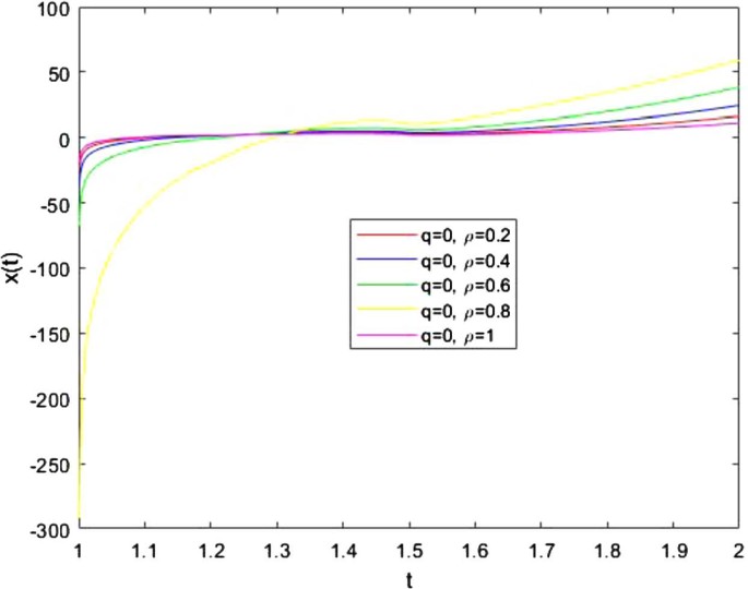
Graph of \(x(t)\), for the Riemann–Liouville fractional derivatives (\(q=0\), \(\rho =1\)), and generalized proportional fractional derivatives (\(q=0\), \(\rho \in (0,1)\))
-
If \(\rho \rightarrow 1\) and \(q=1\), we obtain the Caputo fractional derivative [32].
-
If \(\rho \in (0, 1)\) and \(q=0\), we obtain the Riemann–Liouville generalized proportional fractional derivative [23], which we can see from Fig. 2 to cover the Riemann–Liouville fractional derivative.
-
If \(\rho \in (0, 1)\) and \(q=1\), we obtain the Caputo generalized proportional fractional derivative [23].
-
If \(q,\rho \in (0, 1)\), it is easily to observe from Fig. 3 that the newly proposed derivative unifies the ones in the setting of the Hilfer, Riemann–Liouville and generalized proportional fractional derivatives.
Figure 3 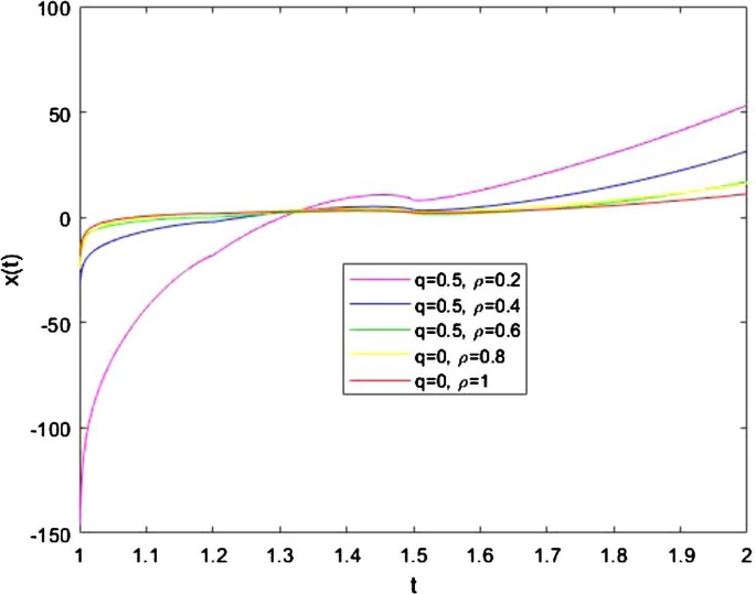
Graph of \(x(t)\), for the Riemann–Liouville fractional derivatives (\(q=0\), \(\rho =1\)), generalized proportional fractional derivatives (\(q=0\), \(\rho =0.8\)) and Hilfer generalized proportional fractional derivatives (\(q\in (0,1)\), \(\rho \in (0,1)\))


4 Conclusions
In this paper, we defined the proportional fractional derivatives in the Hilfer setting. We used some known theorems from the fixed point theory that enabled us to prove the existence and uniqueness of solutions to a specific type of fractional initial value problem involving the Hilfer proportional fractional derivative. Furthermore, to show the effectiveness of our results, we presented some examples. In fact, the Hilfer proportional derivative contains three parameters. The existence of more parameters is useful especially when one considers the stability and other qualitative aspects of differential equations involving fractional derivative.
References
Abdeljawad, T.: On conformable fractional calculus. J. Comput. Appl. Math. 279, 57–66 (2015)
Ahmed, I., Kumam, P., Jarad, F., Borisut, P., Sitthithakerngkiet, K., Ibrahim, A.: Stability analysis for boundary value problems with generalized nonlocal condition via Hilfer–Katugampola fractional derivative. Adv. Differ. Equ. 2020(1), 225 (2020)
Ahmed, I., Kumam, P., Shah, K., Borisut, P., Sitthithakerngkiet, K., Demba, M.A.: Stability results for implicit fractional pantograph differential equations via ϕ-Hilfer fractional derivative with a nonlocal Riemann–Liouville fractional integral condition. Mathematics 8(1), 94 (2020)
Almeida, R.: A Caputo fractional derivative of a function with respect to another function. Commun. Nonlinear Sci. Numer. Simul. 44, 460–481 (2017)
Anatoly, A.K.: Hadamard-type fractional calculus. J. Korean Math. Soc. 38(6), 1191–1204 (2001)
Anderson, D.: Second-order self-adjoint differential equations using a proportional-derivative controller. Commun. Appl. Nonlinear Anal. 24(1), 17–48 (2017)
Anderson, D.R., Ulness, D.J.: Newly defined conformable derivatives. Adv. Dyn. Syst. Appl. 10(2), 109–137 (2015)
Asawasamrit, S., Kijjathanakorn, A., Ntouyas, S.K., Tariboon, J.: Nonlocal boundary value problems for Hilfer fractional differential equations. Bull. Korean Math. Soc. 55(6), 1639–1657 (2018)
Atangana, A.: Derivative with a New Parameter: Theory, Methods and Applications. Academic Press, San Diego (2015)
Atangana, A.: Fractional Operators with Constant and Variable Order with Application to Geo-Hydrology. Academic Press, San Diego (2017)
Atangana, A., Baleanu, D.: Application of fixed point theorem for stability analysis of a nonlinear Schrodinger with Caputo–Liouville derivative. Filomat 31(8), 2243–2248 (2017)
Atangana, A., Baleanu, D., Alsaedi, A.: New properties of conformable derivative. Open Math. 13, 889–898 (2015)
Atangana, A., Goufo, E.F.D.: Cauchy problems with fractal-fractional operators and applications to groundwater dynamics. Fractals (2020, in press). https://doi.org/10.1142/S0218348X20400435
Atangana, A., Koca, I.: New direction in fractional differentiation. Math. Nat. Sci. 1, 18–25 (2017)
Atangana, A., Secer, A.: A note on fractional order derivatives and table of fractional derivatives of some special functions. In: Abstract and Applied Analysis, vol. 2013. Hindawi (2013)
Borisut, P., Kumam, P., Ahmed, I., Sitthithakerngkiet, K.: Nonlinear Caputo fractional derivative with nonlocal Riemann–Liouville fractional integral condition via fixed point theorems. Symmetry 11(6), 829 (2019)
Debnath, L.: Recent applications of fractional calculus to science and engineering. Int. J. Math. Math. Sci., 54, 3413–3442 (2003)
Furati, K.M., Kassim, M.D., et al.: Existence and uniqueness for a problem involving Hilfer fractional derivative. Comput. Math. Appl. 64(6), 1616–1626 (2012)
Gambo, Y.Y., Jarad, F., Baleanu, D., Abdeljawad, T.: On Caputo modification of the Hadamard fractional derivatives. Adv. Differ. Equ. 2014, 10 (2014)
Harikrishnan, S., Shah, K., Baleanu, D., Kanagarajan, K.: Note on the solution of random differential equations via ψ-Hilfer fractional derivative. Adv. Differ. Equ., 2018, 224 (2018)
Hilfer, R., et al.: Applications of Fractional Calculus in Physics, vol. 35. World Scientific, Singapore (2000)
Jarad, F., Abdeljawad, T.: Generalized fractional derivatives and Laplace transform. Discrete Contin. Dyn. Syst., Ser. S 13(3), 709–722 (2020)
Jarad, F., Abdeljawad, T., Alzabut, J.: Generalized fractional derivatives generated by a class of local proportional derivatives. Eur. Phys. J. Spec. Top. 226(16–18), 3457–3471 (2017)
Jarad, F., Abdeljawad, T., Baleanu, D.: Caputo-type modification of the Hadamard fractional derivatives. Adv. Differ. Equ. 2012(1), 142 (2012)
Jarad, F., Abdeljawad, T., Baleanu, D.: On the generalized fractional derivatives and their Caputo modification. J. Nonlinear Sci. Appl. 10(5), 2607–2619 (2017)
Jarad, F., Harikrishnan, S., Shah, K., Kanagarajan, K.: Existence and stability results to a class of fractional random implicit differential equations involving a generalized Hilfer fractional derivative. Discrete Contin. Dyn. Syst., Ser. S 13(3), 723 (2020)
Jarad, F., Uğurlu, E., Abdeljawad, T., Baleanu, D.: On a new class of fractional operators. Adv. Differ. Equ. 2017, 247 (2017)
Katugampola, U.N.: New approach to a generalized fractional integral. Appl. Math. Comput. 218(3), 860–865 (2011)
Katugampola, U.N.: A new approach to generalized fractional derivatives. Bull. Math. Anal. Appl. 6(4), 1–15 (2014)
Khalil, R., Al Horani, M., Yousef, A., Sababheh, M.: A new definition of fractional derivative. J. Comput. Appl. Math. 264, 65–70 (2014)
Khan, M.A., Atangana, A.: Modeling the dynamics of novel coronavirus (2019-ncov) with fractional derivative. Alex. Eng. J. (2020, in press). https://doi.org/10.1016/j.aej.2020.02.033
Kilbas, A., Srivastava, H., Trujillo, J.: Theory and Applications of Fractional Derivatial Equations. North-Holland Mathematics Studies, vol. 204. North-Holland, Amsterdam (2006)
Krasnoselskii, M.: Two remarks about the method of successive approximations. Usp. Mat. Nauk 10, 123–127 (1955)
Magin, R.L.: Fractional Calculus in Bioengineering, vol. 2. Begell House, Redding (2006)
Mainardi, F.: Fractional Calculus and Waves in Linear Viscoelasticity: An Introduction to Mathematical Models. World Scientific, Singapore (2010)
Oliveira, D., de Oliveira, E.C.: Hilfer–Katugampola fractional derivatives. Comput. Appl. Math. 37(3), 3672–3690 (2018)
Osler, T.J.: The fractional derivative of a composite function. SIAM J. Math. Anal. 1(2), 288–293 (1970)
Owolabi, K.M., Atangana, A., Akgul, A.: Modelling and analysis of fractal-fractional partial differential equations: application to reaction–diffusion model. Alex. Eng. J. (2020, in press). https://doi.org/10.1016/j.aej.2020.03.022
Podlubny, I.: Fractional Differential Equations: An Introduction to Fractional Derivatives, Fractional Differential Equations, to Methods of Their Solution and Some of Their Applications, vol. 198. Elsevier, Amsterdam (1998)
Riaz, M.B., Atangana, A., Abdeljawad, T.: Local and nonlocal differential operators: a comparative study of heat and mass transfer in mhd oldroyd-b fluid with ramped wall temperature. Fractals (2020, in press). https://doi.org/10.1142/S0218348X20400332
Samko, S.G., Kilbas, A.A., Marichev, O.I., et al.: Fractional Integrals and Derivatives, vol. 1993. Gordon & Breach, Yverdon (1993)
Shah, K., Vivek, D., Kanagarajan, K.: Dynamics and stability of ψ-fractional pantograph equations with boundary conditions. Bol. Soc. Parana. Mat. 22(2), 1–13 (2018)
Shammakh, W., Alzumi, H.Z.: Existence results for nonlinear fractional boundary value problem involving generalized proportional derivative. Adv. Differ. Equ. 2019, 94 (2019)
Vivek, D., Kanagarajan, K., Elsayed, E.: Some existence and stability results for Hilfer-fractional implicit differential equations with nonlocal conditions. Mediterr. J. Math. 15(1), 15 (2018)
Vivek, D., Shah, K., Kanagarajan, K.: Existence theory and continuation analysis of nonlinear pantograph equations via Hilfer–Hadamard fractional derivative. Dyn. Contin. Discrete Impuls. Syst., Ser. A Math. Anal. 25, 397–417 (2018)
Acknowledgements
The authors acknowledge the financial support provided by the Center of Excellence in Theoretical and Computational Science (TaCS-CoE), KMUTT. The first and last authors were supported by the “Petchra Pra Jom Klao Ph.D. Research Scholarship from King Mongkut’s University of Technology Thonburi”. (For Ph.D. Petchra Pra Jom Klao Doctoral Scholarship) (Grant No. 13/2561). Moreover, this research work was financially supported by King Mongkut’s University of Technology Thonburi through the KMUTT 55th Anniversary Commemorative Fund.
Availability of data and materials
Data sharing is not applicable to this paper, as no data set was generated or analyzed during the current study.
Funding
Petchra Pra Jom Klao Doctoral Scholarship for Ph.D. program of King Mongkut’s University of Technology Thonburi (KMUTT). The Center of Excellence in Theoretical and Computational Science (TaCS-CoE), KMUTT.
Author information
Authors and Affiliations
Contributions
In writing this article the authors have contributed equally. Both authors read and approved the final manuscript.
Corresponding author
Ethics declarations
Competing interests
The authors declare no conflict of interest.
Rights and permissions
Open Access This article is licensed under a Creative Commons Attribution 4.0 International License, which permits use, sharing, adaptation, distribution and reproduction in any medium or format, as long as you give appropriate credit to the original author(s) and the source, provide a link to the Creative Commons licence, and indicate if changes were made. The images or other third party material in this article are included in the article’s Creative Commons licence, unless indicated otherwise in a credit line to the material. If material is not included in the article’s Creative Commons licence and your intended use is not permitted by statutory regulation or exceeds the permitted use, you will need to obtain permission directly from the copyright holder. To view a copy of this licence, visit http://creativecommons.org/licenses/by/4.0/.
About this article

Cite this article
Ahmed, I., Kumam, P., Jarad, F. et al. On Hilfer generalized proportional fractional derivative. Adv Differ Equ 2020, 329 (2020). https://doi.org/10.1186/s13662-020-02792-w
Received:
Accepted:
Published:
DOI: https://doi.org/10.1186/s13662-020-02792-w