
Abstract
In this paper, we use an Ornstein–Uhlenbeck process to describe the environmental stochasticity and propose a stochastic predator–prey model with modified Leslie–Gower and Holling-type II schemes. For each species, sharp sufficient conditions for persistence in the mean and extinction are respectively obtained. The results demonstrate that the persistence and extinction of the species have close relationships with the environmental stochasticity. In addition, the theoretical results are numerically illustrated by some simulations.
1 Introduction
The well-known predator–prey framework with modified Leslie–Gower and Holling-type II schemes (PPFMLHS) formulated by Aziz-Alaoui and Okiye [1] can be illustrated as follows:
where a, c, f and h are assumed to be positive constants. a means the intraspecific competition strength, c measures the per capita reduction rate, h characterises the safeguard of the environment and f possesses the like signification of c. In the past two decades, model (1) and its generalisations have been subjected to intensive research, and a mass of attractive features have been provided. For example, Aziz-Alaoui and Okiye [1] tested the boundedness and global stability of model (1); Guo and Song [2] dissected model (1) perturbed by the impulse; Abid et al. [3] probed into the optimal control of model (1); see [3–15] for more related outcomes.
The parameters in model (1) are hypothesised to be deterministic, which neglects the environmental perturbations, and hence model (1) cannot accurately depict the real situations. A mass of scholars (see [16–23]) introduced stochasticity into deterministic systems to dissect the functions of stochasticity on population dynamics. Particularly, under the hypothesis that the growth rates in model (1) are disturbed by the random perturbations with \(r_{i}\rightarrow r_{i}+\sigma _{i}\frac{\mathrm{d}B_{i}(t)}{dt}\), several authors (see [16–18, 20]) tested the following stochastic PPFMLHS:
where \(\sigma _{i}^{2}\) means the intensity of white noise, \(B_{i}(t)\) is a standard Brownian motion defined on \((\varOmega ,\mathcal{F}_{t}, P)\), a given complete probability space. Ji et al. [17, 18] probed into several dynamical characteristics of system (2) and offered extinct and persistent conditions for the system. Liu et al. [20] examined the persistence and extinction of model (2) with impulsive toxicant input.
Model (2) hypothesises that the growth rate in the random environments is linear with respect to the Gaussian white noise
Integrating on the interval \([0,T]\) results in
Therefore, the variance of the average per capita growth rate \(\overline{r}_{i}\) over an interval of length T tends to ∞ as \(T \rightarrow 0\). This is insufficient to describe the real situation. Several authors (see [24, 25]) have claimed that using the mean-reverting Ornstein–Uhlenbeck process is a more appropriate approach to incorporate the environmental perturbations. On account of this approach, one has
i.e.
where \(r_{i0}=\tilde{r}_{i}(0)\), \(\sigma _{i}(t)=\frac{\xi _{i}}{\sqrt{2\alpha _{i}}}\sqrt{1-e^{-2 \alpha _{i} t}}\), \(\alpha _{i}>0\) characterises the speed of reversion, \(\xi _{i}^{2}\) means the intensity of stochastic perturbations. We then derive the following stochastic PPFMLHS:
As far as we know, little research has been conducted to explore model (3). For this reason, we delve into the properties of model (3).
The arrangement of this paper is as follows. In Sect. 2, the persistence and extinction threshold for each population are proffered. In Sect. 3, some numerical simulations are performed to evidence the theoretical outcomes. In Sect. 4, a number of concluding remarks are put forward.
2 Main results
Define
Lemma 1
For arbitrary\((x(0),y(0))\in R_{+}^{2}\), model (3) possesses a unique solution\((x(t),y(t))\in R_{+}^{2}\)for all\(t\geq 0\)a.s. (almost surely).
Proof
Pay attention to the following system:
and \(u(0)=\ln {x(0)}\), \(v(0)=\ln {y(0)}\). Due to the fact that the coefficients of system (4) adhere to the Lipschitz condition, system (4) possesses a unique local solution \((u(t), v(t))\) on \([0, \tau _{*})\) (see Theorems 3.15–3.17 in [26]), where \(\tau _{*}\) means the explosion time. Then we can deduce from Itô’s formula that on \([0, \tau _{*})\) model (3) possesses a unique solution \((x(t),y(t))=(e^{u(t)},e^{v(t)})\) which is positive. Now we validate \(\tau _{*}= +\infty \). Focus on the following systems:
On the basis of the comparison theorem [27], for \(t\in [0,\tau _{*})\),
In accordance to Theorem 2.2 in [22],
and
Due to the fact that \(\varPhi (t)\), \(\psi (t)\), \(\varphi (t)\) are global, we can deduce that \(\tau _{*}=+\infty \). □
Lemma 2
([28])
Let\(\varGamma (t)\in C(\varOmega \times [0,+\infty ),[0,+\infty ))\).
- (I)
If one can find out three positive constantsκ, μand\(\mu _{0}\)such that, for all\(t \geq \kappa \), \(\ln {\varGamma (t)}\leq \mu {t}-\mu _{0}{\int _{0}^{t} \varGamma (s) \,\mathrm{d}s}+F(t)\), where\(F(t)/t\rightarrow 0\)as\(t\rightarrow +\infty \), then\(\limsup_{t \to +\infty }{t^{-1}\int _{0}^{t}\varGamma (s) \,\mathrm{d}s} \leq \frac{\mu }{\mu _{0}}\)a.s.
- (II)
If one can find out three positive constantsκ, μand\(\mu _{0}\)such that, for all\(t \geq \kappa \), \(\ln {\varGamma (t)}\geq \mu {t}-\mu _{0}{\int _{0}^{t}\varGamma (s) \,\mathrm{d}s}+F(t)\), where\(F(t)/t\rightarrow 0\)as\(t\rightarrow +\infty \), then\(\liminf_{t\to +\infty }{t^{-1}\int _{0}^{t} \varGamma (s) \,\mathrm{d}s} \geq \frac{\mu }{\mu _{0}}\)a.s.
Lemma 3
If\(\bar{b}_{1}>0\)and\(\bar{b}_{2}>0\), then\(\lim_{t\to +\infty }t^{-1}\ln {y(t)}=0\)a.s.
Proof
Choose sufficiently large T which fulfils that, for \(t \geq T\),
For \(t \geq T\), one can deduce from (9) that
where
It then follows from \(L_{1}(t)\geq 1\) that
where
Thus (11) implies that
where
For this reason,
We then deduce from \(\lim_{t\to +\infty }t^{-1}\int _{0}^{t} {\sigma _{i}(s)\,\mathrm{d}B_{i}(s)}=0\) (\(i=1, 2\)) that if \(\bar{b}_{2}>0\),
This, together with (12), indicates
Taking advantage of Itô’s formula to (6) deduces
namely,
For arbitrary \(\varepsilon >0\), one can find out \(T>0\) such that, for \(t\geq T\),
We then deduce from (13) that, for \(t\geq T\),
Choose \(0<\varepsilon <\bar{b}_{2}\). Making use of (I) and (II) in Lemma 2 yields that
We then deduce from the arbitrariness of ε that
which indicates that \(\lim_{t\to +\infty }{t^{-1}\ln {\psi (t)}}=0\) a.s. In accordance to (8),
□
Theorem 1
([28])
For model (3), the following conclusions hold:
- (i)
If\(\bar{b}_{1}<0\), \(\bar{b}_{2}<0\), then bothxandybecome extinct, i.e. \(\lim_{t\to +\infty }x(t)=0\), \(\lim_{t\to +\infty }y(t)=0\)a.s.
- (ii)
If\(\bar{b}_{1} < 0\), \(\bar{b}_{2} >0\), thenxbecomes extinct andyis persistent in the mean, i.e. \(\lim_{t\to +\infty }{t^{-1}\int _{0}^{t} y(s)\,\mathrm{d}s}=h\bar{b}_{2}/f\)a.s.
- (iii)
If\(\bar{b}_{1} > 0\), \(\bar{b}_{2}<0\), thenybecomes extinct andxis persistent in the mean, i.e. \(\lim_{t\to +\infty }{t^{-1}\int _{0}^{t}x(s)\,\mathrm{d}s}= \bar{b}_{1}/a\)a.s.
- (iv)
When\(\bar{b}_{1}>0\), \(\bar{b}_{2}>0\), (a) if\(\bar{b}_{1}< c\bar{b}_{2}/f\), thenxbecomes extinct andyis persistent in the mean, i.e. \(\lim_{t\to +\infty }{t^{-1}\int _{0}^{t}y(s)\,\mathrm{d}s}=h\bar{b}_{2}/f\)a.s.; (b) if\(\bar{b}_{1} >c\bar{b}_{2}/f\), then\(\lim_{t\to +\infty }{t^{-1}\int _{0}^{t} x(s)\,\mathrm{d}s}=\bar{b}_{1}/a-c \bar{b}_{2}/(af)\), \(\lim_{t\to +\infty }{t^{-1}\int _{0}^{t}{\frac{y(s)}{h+x(s)}} \,\mathrm{d}s}=\bar{b}_{2}/f\)a.s.
Proof
(i). Taking advantage of Itô’s formula to (3) results in
As a consequence,
We then deduce from (18) that, for sufficiently large t,
In accordance to \(\lim_{t\to +\infty }t^{-1}\int _{0}^{t}\sigma _{1}(s)\,\mathrm{d}B_{1}(s)=0\) and \(\bar{b}_{1}+\varepsilon <0\), we derive \(\lim_{t\to +\infty }x(t)=0\) a.s. Analogously, \(\bar{b}_{2}<0\) means that \(\lim_{t\to +\infty }y(t)=0\) a.s.
(ii). Note that \(\bar{b}_{1}<0\), hence (i) indicates that \(\lim_{t\to +\infty }x(t)=0\). As a result, for sufficiently large t,
Making use of Lemma 2 to (21) and (22) results in
We then deduce from the arbitrariness of ε that \(\lim_{t\to +\infty }{t^{-1}\int _{0}^{t}y(s)\,\mathrm{d}s}=h\bar{b}_{2}/f\) a.s.
(iii). Since \(\bar{b}_{2}<0\), then analogous to the proof of (i), one can validate that \(\lim_{t\to +\infty }y(t)=0\). The proof of (iii) is analogous to that of (ii), thus is left out.
(iv). (a). Compute that \(\text{(18)}\times f-\text{(19)}\times c\),
On the basis of Lemma 3, for arbitrary \(\varepsilon >0\), we can find out \(T>0\) such that, for \(t\geq T\), \(ct^{-1}\ln {\frac{y(t)}{y(0)}}\leq \varepsilon /5\). For this reason,
As a result, for \(t\geq T\),
Choose \(0<\varepsilon < c\bar{b}_{2}-f\bar{b}_{1}\). Consequently, \(\lim_{t\to +\infty }x(t)=0\). The proof of
is analogous to that of (ii) and thereby is left out.
(b). On the basis of (19),
We then deduce from Lemma 3 and \(\lim_{t\to +\infty }t^{-1}\int _{0}^{t}\sigma _{2}(s)\,\mathrm{d}B_{2}(s)=0\) that
As a consequence, for any \(\varepsilon >0\), we can find out \(T>0\) such that, for \(t\geq T\),
Applying (26) to (18) gives that, for \(t\geq T\),
Choose \(0<\varepsilon <(\bar{b}_{1}-c\bar{b}_{2}/f)/2\). On the basis of Lemma 2,
We then deduce from the arbitrariness of ε that \(\lim_{t\to +\infty }{t^{-1}\int _{0}^{t}x(s)\,\mathrm{d}s}=\bar{b}_{1}/a-c \bar{b}_{2}/(af)\). □
3 Discussions and numerical simulations
Now we test the functions of the mean-reverting Ornstein–Uhlenbeck process on the persistence and extinction of model (3). There are two key parameters in the Ornstein–Uhlenbeck process: the speed of reversion \(\alpha _{i}\) and the intensity of the perturbation \(\xi _{i}\). In light of Theorem 1, the persistence and extinction of system (3) are entirely dominated by the signs of \(\bar{b}_{1}\), \(\bar{b}_{2}\) and \(\bar{b}_{1}-c\bar{b}_{2}/f\). Clearly,
For this reason, with the rise of \(\alpha _{i}\) (respectively, \(\xi _{i}\)), species i tends to be persistent (respectively, extinct), \(i=1,2\). Furthermore, due to the fact that \(\frac{\partial (\bar{b}_{1}-c\bar{b}_{2}/f)}{\partial \alpha _{2}}<0\) (respectively, \(\frac{\partial (\bar{b}_{1}-c\bar{b}_{2}/f)}{\partial (\xi _{2}^{2})}>0\)), thus sufficiently large \(\alpha _{2}\) (respectively, \(\xi _{2}\)) could make the prey population extinct (respectively, persistent) provided \(\bar{b}_{1}>0\) and \(\bar{b}_{2}>0\).
Now we numerically validate the above outcomes (here we only provide the functions of \(\alpha _{i}\) since the functions of \(\xi _{i}\) can be proffered analogously). On the basis of the Milstein method offered in [29], model (3) can be discretized as follows:
where \(\xi ^{k}\), \(\eta ^{k}\), \(k = 1, 2, \ldots , K\), mean independent Gaussian random variables.
Choose \(r_{1}=0.6\), \(r_{2}=0.4\), \(r_{10}=0.3\), \(r_{20}=0.2\), \(\xi _{1}^{2}=1.43\), \(\xi _{2}^{2}=0.63\), \(a=0.4\), \(c=0.36\), \(f=0.25\), \(h=1\) (these and the following parameter values are hypothesised). Now, we let \(\alpha _{1}\) and \(\alpha _{2}\) vary.
Choose \(\alpha _{1} =0.55\), \(\alpha _{2}= 0.35\). Then \(\bar{b}_{1}=-0.05\), \(\bar{b}_{2}=-0.05\). On the basis of (i) in Theorem 1, both x and y become extinct. See Fig. 1.
Figure 1 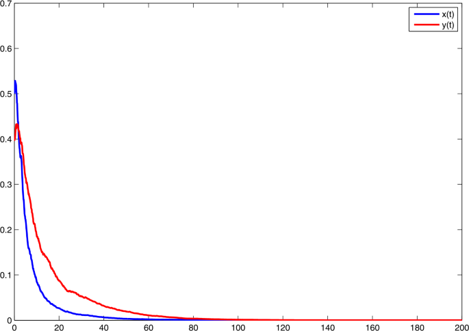
Solutions of model (3) with \(r_{1}=0.6\), \(r_{2}=0.4\), \(r_{10}=0.3\), \(r_{20}=0.2\), \(\xi _{1}^{2}=1.43\), \(\xi _{2}^{2}=0.63\), \(a=0.4\), \(c=0.36\), \(f=0.25\), \(h=1\). With \(\alpha _{1} =0.55\), \(\alpha _{2}= 0.35\)
Choose \(\alpha _{1}=0.55\), \(\alpha _{2}=0.525\). Then \(\bar{b}_{1}=-0.05\), \(\bar{b}_{2}=0.1\). On the basis of (ii) in Theorem 1, x becomes extinct and \(\lim_{t\to +\infty }{t^{-1}\int _{0}^{t}y(s)\,\mathrm{d}s}=h\bar{b}_{1}/f=0.4\). See Fig. 2.
Figure 2 
Solutions of model (3) with \(r_{1}=0.6\), \(r_{2}=0.4\), \(r_{10}=0.3\), \(r_{20}=0.2\), \(\xi _{1}^{2}=1.43\), \(\xi _{2}^{2}=0.63\), \(a=0.4\), \(c=0.36\), \(f=0.25\), \(h=1\). With \(\alpha _{1} =0.55\), \(\alpha _{2}= 0.525\)
Choose \(\alpha _{1}=0.65\), \(\alpha _{2}=0.35\). Then \(\bar{b}_{1}=0.05\), \(\bar{b}_{2}=-0.05\). On the basis of (iii) in Theorem 1, y becomes extinct and \(\lim_{t\to +\infty }{t^{-1}\int _{0}^{t}x(s)\,\mathrm{d}s}=\bar{b}_{1}/a=0.125\). See Fig. 3. Comparing Fig. 1 with Fig. 2, one could perceive that with the rise of \(\alpha _{2}\), the predator population inclines to be persistent. Analogously, comparing Fig. 1 with Fig. 3, one could perceive that with the rise of \(\alpha _{1}\), the prey population inclines to be persistent.
Figure 3 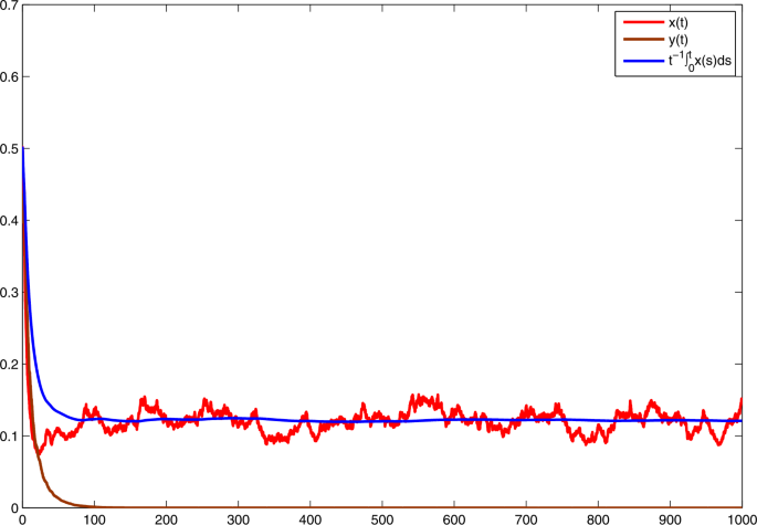
Solutions of model (3) with \(r_{1}=0.6\), \(r_{2}=0.4\), \(r_{10}=0.3\), \(r_{20}=0.2\), \(\xi _{1}^{2}=1.43\), \(\xi _{2}^{2}=0.63\), \(a=0.4\), \(c=0.36\), \(f=0.25\), \(h=1\). With \(\alpha _{1} =0.65\), \(\alpha _{2}= 0.35\)
Choose \(\alpha _{1}=0.715\), \(\alpha _{2}=0.7875\). Then \(\bar{b}_{1}=0.1\), \(\bar{b}_{1}=0.2\), \(\bar{b}_{1}< c\bar{b}_{2}/f=0.288\). On the basis of (a) in Theorem 1, x becomes extinct and \(\lim_{t\to +\infty }{t^{-1}\int _{0}^{t}y(s)\,\mathrm{d}s} =h\bar{b}_{2}/f=0.8\). See Fig. 4.
Figure 4 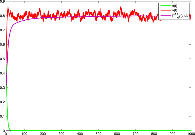
Solutions of model (3) with \(r_{1}=0.6\), \(r_{2}=0.4\), \(r_{10}=0.3\), \(r_{20}=0.2\), \(\xi _{1}^{2}=1.43\), \(\xi _{2}^{2}=0.63\), \(a=0.4\), \(c=0.36\), \(f=0.25\), \(h=1\). With \(\alpha _{1} =0.715\), \(\alpha _{2}= 0.7875\)
Choose \(\alpha _{1} =0.715\), \(\alpha _{2}= 0.45\). Then \(\bar{b}_{1}=0.1\), \(\bar{b}_{2}=0.05\), \(\bar{b}_{1}>c\bar{b}_{2}/f=0.072\). On the basis of (b) in Theorem 1, \(\lim_{t\to +\infty }{t^{-1}\int _{0}^{t}x(s)\,\mathrm{d}s}=\bar{b}_{1}/a-c \bar{b}_{2}/(af)=0.07\). \(\lim_{t\to +\infty }{t^{-1}\int _{0}^{t}{\frac{y(s)}{h+x(s)}} \,\mathrm{d}s}=\bar{b}_{2}/f=0.2\). See Fig. 5. In comparison with Fig. 4, one could perceive that with the rise of \(\alpha _{2}\), the prey population inclines to become extinct.
Figure 5 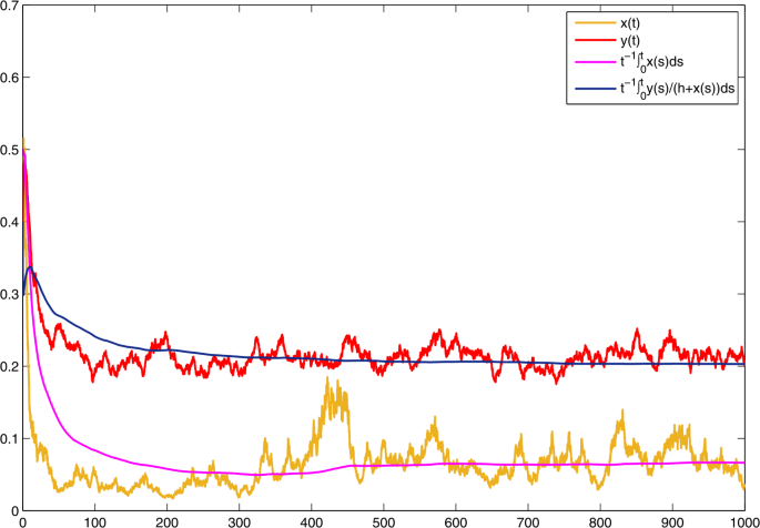
Solutions of model (3) with \(r_{1}=0.6\), \(r_{2}=0.4\), \(r_{10}=0.3\), \(r_{20}=0.2\), \(\xi _{1}^{2}=1.43\), \(\xi _{2}^{2}=0.63\), \(a=0.4\), \(c=0.36\), \(f=0.25\), \(h=1\). With \(\alpha _{1} =0.715\), \(\alpha _{2}= 0.45\)


4 Concluding remarks
In the present article, we took advantage of a mean-reverting Ornstein–Uhlenbeck process to portray the random perturbations in the environment and formulated a stochastic PPFMLHS which might be more appropriate than model (2). We offered the persistence-and-extinction threshold of the model and uncovered some significant functions of Ornstein–Uhlenbeck process: sufficiently large \(\alpha _{i}\) (the speed of reversion) could make species i persistent; furthermore, in some cases sufficiently large \(\alpha _{2}\) could make species 1 (the prey population) become extinct.
Several problems remain to be solved. First, the present article tests the predator–prey framework, it would be interesting to dissect the food-chain framework (see [30]). Second, the present article probed into the white noises, one could examine other random noises such as the telephone noise (see [31]), the Lévy noise (see [32]) etc. When the telephone noise is considered, model (3) is replaced with
where \(\lambda (t)\) is a Markov chain with finite states. When the Lévy noise is considered, model (3) is replaced with
where \(\mu (t^{-})\) means the left limit of \(\mu (t)\), Γ̃ is the compensating measure of a Poisson measure Γ, \(\varXi \subseteq (0,+\infty )\) adheres to \(\gamma (\varXi )<+\infty \), where γ is the characteristic measure of Γ̃. Finally, one could take the intraspecific competition of the predator population into account, which was neglected in model (3).
References
Aziz-Alaoui, M.A., Okiye, M.D.: Boundedness and global stability for a predator–prey model with modified Leslie–Gower and Holling-type II schemes. Appl. Math. Lett. 16, 1069–1075 (2003)
Guo, H.J., Song, X.Y.: An impulsive predator–prey system with modified Leslie–Gower and Holling type II schemes. Chaos Solitons Fractals 36, 1320–1331 (2008)
Abid, W., Yafia, R., Aziz-Alaoui, M.A., Aghriche, A.: Dynamics analysis and optimality in selective harvesting predator–prey model with modified Leslie–Gower and Holling-type II. Nonauton. Dyn. Syst. 6, 1–17 (2019)
Banerjee, M., Banerjee, S.: Turing instabilities and spatio-temporal chaos in ratio-dependent Holling–Tanner model. Math. Biosci. 236, 64–76 (2012)
Chen, F.D., Chen, L.J., Xie, X.D.: On a Leslie–Gower predator–prey model incorporating a prey refuge. Nonlinear Anal., Real World Appl. 10, 2905–2908 (2009)
Tian, Y.L., Weng, P.X.: Stability analysis of diffusive predator–prey model with modified Leslie–Gower and Holling-type III schemes. Appl. Math. Comput. 218, 3733–3745 (2011)
Song, X.Y., Li, Y.F.: Dynamic behaviors of the periodic predator–prey model with modified Leslie–Gower Holling-type II schemes and impulsive effect. Nonlinear Anal., Real World Appl. 9, 64–79 (2008)
Yafia, R., Adnani, F., Alaoui, H.T.: Limit cycle and numerical simulations for small and large delays in a predator–prey model with modified Leslie–Gower and Holling-type II schemes. Nonlinear Anal., Real World Appl. 9, 2055–2067 (2008)
Nie, L.F., Teng, Z.D., Hu, L., Peng, J.G.: Qualitative analysis of a modified Leslie–Gower and Holling-type II predator–prey model with state dependent impulsive effects. Nonlinear Anal., Real World Appl. 11, 1364–1373 (2010)
Nindjin, A.F., Aziz-Alaoui, M.A., Cadivel, M.: Analysis of a predator–prey model with modified Leslie–Gower and Holling-type II schemes with time delay. Nonlinear Anal., Real World Appl. 7, 1104–1118 (2006)
Ali, N., Jazar, M.: Global dynamics of a modified Leslie–Gower predator–prey model with Crowley–Martin functional responses. Appl. Math. Comput. 43, 271–293 (2013)
Ghaziania, R.K., Alidousti, J., Eshkaftaki, A.B.: Stability and dynamics of a fractional order Leslie–Gower prey-predator model. Appl. Math. Model. 40, 2075–2086 (2016)
Zhou, J., Kim, C., Shi, J.G.: Positive steady state solutions of a diffusive Leslie–Gower predator–prey model with Holling type II functional response and cross-diffusion. Dyn. Syst. 34, 3875–3899 (2014)
Cao, J.Z., Yuan, R.: Bifurcation analysis in a modified Leslie–Gower model with Holling type II functional response and delay. Nonlinear Dyn. 84, 1341–1352 (2016)
Guan, X.N., Wang, W.M., Cai, Y.L.: Spatiotemporal dynamics of a Leslie–Gower predator–prey model incorporating a prey refuge. Nonlinear Anal., Real World Appl. 12, 2385–2395 (2011)
Xu, Y., Liu, M., Yang, Y.: Analysis of a stochastic two-predators one-prey system with modified Leslie–Gower and Holling-type II schemes. J. Appl. Anal. Comput. 7, 713–727 (2017)
Ji, C.Y., Jiang, D.Q., Shi, N.Z.: Analysis of a predator–prey model with modified Leslie–Gower and Holling type II schemes with stochastic perturbation. J. Math. Anal. Appl. 359, 482–498 (2009)
Ji, C.Y., Jiang, D.Q., Shi, N.Z.: A note on a predator–prey model with modified Leslie–Gower and Holling-type II schemes with stochastic perturbation. J. Math. Anal. Appl. 377, 435–440 (2011)
Zou, X.L., Fan, D.J., Wang, K.: Stationary distribution and stochastic Hopf bifurcation for a predator–prey system with noises. Discrete Contin. Dyn. Syst., Ser. B 18, 1507–1519 (2013)
Liu, M., Du, C.X., Deng, M.L.: Persistence and extinction of a modified Leslie–Gower Holling-type II stochastic predator–prey model with impulsive toxicant input in polluted environments. Nonlinear Anal. Hybrid Syst. 27, 177–190 (2018)
Beddington, J.R., May, R.M.: Harvesting natural populations in a randomly fluctuating environment. Science 197, 463–465 (1977)
Jiang, D.Q., Shi, N.Z.: A note on non-autonomous logistic equation with random perturbation. J. Math. Anal. Appl. 303, 164–172 (2005)
Li, X.Y., Mao, X.R.: Population dynamical behavior of non-autonomous Lotka–Volterra competitive system with random perturbation. Discrete Contin. Dyn. Syst. 24, 523–545 (2009)
Zhao, Y., Yuan, S.L., Ma, J.L.: Survival and stationary distribution analysis of a stochastic competitive model of three species in a polluted environment. Bull. Math. Biol. 77, 1285–1326 (2015)
Cai, Y.L., Jiao, J.J., Gui, Z.J., Liu, Y.T., Wang, W.M.: Environmental variability in a stochastic epidemic model. Appl. Math. Comput. 329, 210–226 (2018)
Mao, X.R., Yuan, C.G.: Stochastic Differential Equations with Markovian Switching. Imperial College Press, London (2006)
Ikeda, N., Wantanabe, S.: Stochastic Differential Equations and Diffusion Processes. North-Holland, Amsterdam (1981)
Liu, M., Wang, K., Wu, Q.: Survival analysis of stochastic competitive models in a polluted environment and stochastic competitive exclusion principle. Bull. Math. Biol. 73, 1969–2012 (2011)
Higham, D.J.: An algorithmic introduction to numerical simulation of stochastic differential equations. SIAM Rev. 43, 525–546 (2011)
Liu, M., Bai, C.Z.: Analysis of a stochastic tri-trophic food-chain model with harvesting. J. Math. Biol. 73, 597–625 (2016)
Liu, M.: Dynamics of a stochastic regime-switching predator–prey model with modified Leslie–Gower Holling-type II schemes and prey harvesting. Nonlinear Dyn. 96, 417–442 (2019)
Bao, J.H., Mao, X.R., Yin, G., Yuan, C.G.: Competitive Lotka–Volterra population dynamics with jumps. Nonlinear Anal., Real World Appl. 74, 6601–6616 (2011)
Acknowledgements
The authors thank the editor and referees for their careful reading and valuable comments. The authors also thank Prof. Ronghua Tan for the writing instructions.
Availability of data and materials
All data generated or analysed during this study are included in this published article.
Funding
ML thanks the National Natural Science Foundation of China (No. 11771174) and the Natural Science Foundation of Jiangsu Province, China (No. BK20170067), and ZJL thanks the National Natural Science Foundation of China (No. 11871201) and the Natural Science Foundation of Hubei Province, China (No. 2019CFB241). The above foundation items will be used to pay the publication charge.
Author information
Authors and Affiliations
Contributions
DXZ mainly finished the writing of the whole content of the paper. ML and ZJL mainly finished the establishment of model and development. All authors read and approved the final manuscript.
Corresponding author
Ethics declarations
Competing interests
The authors declare that they have no competing interests.
Rights and permissions
Open Access This article is licensed under a Creative Commons Attribution 4.0 International License, which permits use, sharing, adaptation, distribution and reproduction in any medium or format, as long as you give appropriate credit to the original author(s) and the source, provide a link to the Creative Commons licence, and indicate if changes were made. The images or other third party material in this article are included in the article’s Creative Commons licence, unless indicated otherwise in a credit line to the material. If material is not included in the article’s Creative Commons licence and your intended use is not permitted by statutory regulation or exceeds the permitted use, you will need to obtain permission directly from the copyright holder. To view a copy of this licence, visit http://creativecommons.org/licenses/by/4.0/.
About this article

Cite this article
Zhou, D., Liu, M. & Liu, Z. Persistence and extinction of a stochastic predator–prey model with modified Leslie–Gower and Holling-type II schemes. Adv Differ Equ 2020, 179 (2020). https://doi.org/10.1186/s13662-020-02642-9
Received:
Accepted:
Published:
DOI: https://doi.org/10.1186/s13662-020-02642-9