
Abstract
This paper studies the analytical, semi-analytical, and numerical solutions of the Cahn–Allen equation, which plays a vital role in describing the structure of the dynamics for phase separation in Fe–Cr–X (\(X=Mo,Cu\)) ternary alloys. The modified Khater method, the Adomian decomposition method, and the quintic B-spline scheme are implemented on our suggested model to get distinct kinds of solutions. These solutions describe the dynamics of the phase separation in iron alloys and are also used in solidification and nucleation problems. The applications of this model arise in many various fields such as plasma physics, quantum mechanics, mathematical biology, and fluid dynamics. The comparison between the obtained solutions is represented by using figures and tables to explain the value of the error between exact and numerical solutions. All solutions are verified by using Mathematica software.
1 Introduction
The nonlinear partial differential equation (NLPDE) have been considered a fundamental icon in many research ideas. It has been used to formulate many natural, engineering, mechanical, and physical phenomena; this happens because it contains beforehand unknown multi-variable functions and its derivatives. During the last decade, many aspects have been formulated in NLPDE form. Study and investigation of the solitary wave for these models are considered as one of the basic interests of many researchers. The obtained solutions are used to motivate the semi-analytical and numerical schemes to be more accurate. Moreover, the solitary wave is a kind of wave which propagates without any time evolution in shape or size. Many analytical, semi-analytical and numerical schemes have been derived from investigating the physical dynamics of these models such as the Adomian decomposition method, the simplest equation method, modified tanh-function method, B-spline method, iterative method [1–14].
In this context, many nonlinear evolutions equations which represent many important phenomena have been studied and one investigated its properties and dynamical behavior such as by the Benjamin–Bona–Mahony equation, Bateman–Burgers equation, Benjamin–Ono equation, Boomeron equation, Calabi flow equation, Cauchy momentum equation, complex Monge–Ampère equation, Davey–Stewartson equation [15–30].
This research paper focuses on studying the Cahn–Allen equation which is considered as one of the essential models in the plasma physics, quantum mechanics, mathematical biology, and fluid dynamics and describes the dynamics of the phase separation in iron alloys. Moreover, it is also used in solidification and nucleation problems. The Allen–Cahn equation was derived to describe the process of phase separation in multicomponent alloy systems, including order–disorder transitions where it is a reaction–diffusion equation of mathematical physics. This model is given by
where \(\varUpsilon _{\varXi }\), f, Θ, q, \(\varXi _{0}\), m represent the mobility, the free energy density, the control on the state variable at the portion of the boundary \(\partial _{\varXi } \varOmega \), the source control at \(\partial _{q} \varOmega \), the initial condition, and the outward normal to ∂Ω, respectively. This model is also the \(L^{2}\) gradient flow of the Ginzburg–Landau–Wilson free energy functional and close to the Cahn–Hilliard equation.
The Cahn–Allen equation (a.k.a. as Allen–Cahn equation or the Nagumo equation) is given by
where
According to the interfaces that travel upwards in the vertical y direction with a constant speed c, we can rewrite Eq. (2) as
According to the De Giorgi conjecture, the natural extension of Eq. (4) has the following form:
Thus, it is given in the simple form of
The strategy of this paper is summarized as follows: In Sect. 2, we apply the modified Khater method, Adomian decomposition method, and B-spline schemes [31–35] to the Cahn–Allen model [36–39]. In Sect. 3, we study our obtained solutions, showing a novel comparison between our solutions and the other existing results in the available literature. In Sect. 4, we draw a conclusion of all major results.
2 Application
In this section, the analytical, semi-analytical and numerical schemes are applied to our suggested model. Using the wave transformation \(\varXi =\varXi (x,t)=\varXi (\Im )\), \(\Im =k x+\omega t\) on Eq. (6) yields
Using the balance homogeneous rule between the highest order derivatives and nonlinear terms leads to \(n=1\).
2.1 Analytical solution
Applying the modified Khater method on Eq. (7) leads to formulating the general solution form of the Cahn–Allen equation,
where K is arbitrary constant and \(f(\Im )\) is a solution function of the following auxiliary equation:
where β, α, σ are arbitrary constants, which will be determined. Substituting Eq. (8) along with (9) into Eq. (7) and collecting all coefficients of the same power of \(k^{f(\Im )}\) gives an algebraic equation system. Solving the obtained system yields
Thus, the solitary wave solutions of the Cahn–Allen equation according to Family I are given as follows.
When \(\beta ^{2}-4 \alpha \sigma <0\) and \(\sigma \neq 0\)
When \(\beta ^{2}-4 \alpha \sigma >0\) and \(\sigma \neq 0\)
When \(\alpha \sigma <0\) and \(\sigma \neq 0\) and \(\alpha \neq 0\) and \(\beta =0\)
When \(\alpha \sigma >0\) and \(\sigma \neq 0\) and \(\alpha \neq 0\) and \(\beta =0\)
When \(\beta =0\) and \(\alpha =-\sigma \)
When \(\alpha = 0\) and \(\beta \neq 0\) and \(\sigma \neq 0\)
When \(\beta =0\) and \(\alpha =\sigma \)
Meanwhile, the solitary wave solutions of the Cahn–Allen equation according to Family II are given as follows.
When \(\beta ^{2}-4 \alpha \sigma <0\) and \(\sigma \neq 0\)
When \(\beta ^{2}-4 \alpha \sigma >0\) and \(\sigma \neq 0\)
When \(\alpha \sigma <0\) and \(\sigma \neq 0\) and \(\alpha \neq 0\) and \(\beta =0\)
When \(\beta =0\) and \(\alpha =-\sigma \)
When \(\beta =\frac{\alpha }{2}= \kappa \) and \(\sigma =0\)
When \(\beta =0\) and \(\alpha =\sigma \)
When \(\sigma =0\) and \(\beta \neq 0\) and \(\alpha \neq 0\)
2.2 Semi-analytical solution
Applying the Adomian decomposition method on Eq. (7) allows rewriting it as
where L, R, N represent a differential operator, a linear operator and nonlinear term, respectively. Using the inverse operator \(L^{-1}\) on (31), yields
Under the condition \([ \alpha =-1, \beta =0, \sigma =4, \omega =-\frac{3}{8}, k=-\frac{1}{4 \sqrt{2}} ]\) on Eq. (14), we get
So we obtain
According to Eqs. (34)–(36), we get the semi-analytical solution of Eq. (6),
2.3 Numerical solution
This part discusses the numerical solution of the Cahn–Allen equation by using the quintic B-spline. Based on the quintic B-spline, the suggested solution of the ordinary differential of the Cahn–Allen equation is given as
where \(c_{i}\), \(B_{i}\) meet the conditions
and
where \(i \in [-2,n+2]\). Thus, the approximate solution is given as
Substituting Eq. (41) and its derivatives into Eq. (6) yields a system of equations. Solving this system gives the value of \(c_{i}\). Substituting the values of \(c_{i}\), \(B_{i}\) into Eq. (38), one obtains
3 Results and discussion
This section discusses and studies the solutions obtained in (2.1), (2.2), (2.3) to show the novel aspects of our obtained solutions. This study is organized as follows:
- 1.
In Sect. 2.1, the modified Khater method is applied to the Cahn–Allen to get the analytical wave solutions of this equation to study the structure of the dynamics for phase separation in Fe–Cr–X (\(X=Mo, Cu\)) ternary alloys. We compare our obtained solutions with that obtained in [37].
In that paper, Hosseini, Bekir, and Ansari have used the modified Kudryashov method to get the analytical wave solutions of the Cahn–Allen equation, and by focusing on their solutions, we find Eq. (30) is similar to \(u_{1,2}(x,t)\) when \([-\alpha =d, \beta =1, e=a ]\). On the other side, all other obtained solutions in our paper are considered as a different form of solutions of that obtained in [37]. Also, we can see that the modified Khater method gives many different forms of solutions, not like the modified Kudryashov method, and that is considered as a good advantage of the method itself. Moreover, we sketch some results in Figs. 1–6 of our solutions to show more physical properties of the phase separation in Fe–Cr–X (\(X=Mo, Cu\)) ternary alloys.
Figure 1 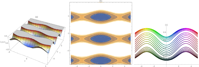
Solitary wave of the Cahn–Allen equation by using Eq. (12) in three- (a), two- (c) dimensional and contour plot (b), when \([\sigma =1, \alpha =2, \beta =3 ]\), which shows the structure of the dynamics for phase separation in Fe–Cr–X (\(X=Mo, Cu\)) ternary alloys
Figure 2 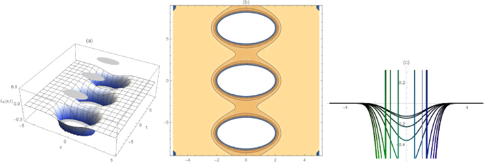
Solitary wave of the Cahn–Allen equation by using Eq. (13) in three- (a), two- (c) dimensional and contour plot (b), when \([\sigma =1, \alpha =2, \beta =3 ]\), which shows the structure of the dynamics for phase separation in Fe–Cr–X (\(X=Mo, Cu\)) ternary alloys
Figure 3 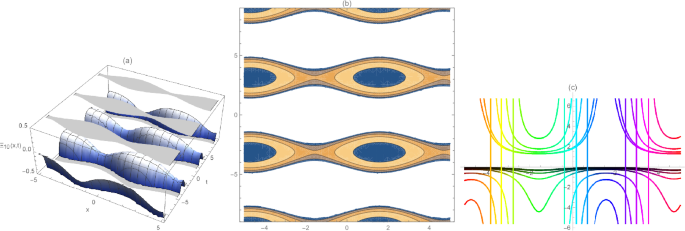
Solitary wave of the Cahn–Allen equation by using Eq. (19) in three- (a), two- (c) dimensional and contour plot (b), when \([\sigma =1, \alpha =0, \beta =3 ]\), which shows the structure of the dynamics for phase separation in Fe–Cr–X (\(X=Mo, Cu\)) ternary alloys
Figure 4 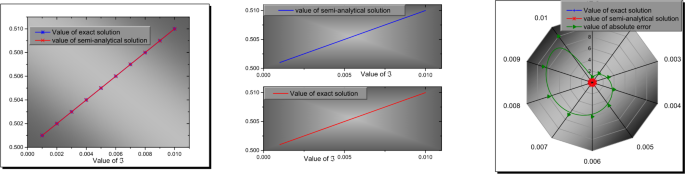
Semi-analytical wave solution of the Cahn–Allen equation by using Eq. (37) in combined, separated, and radar plots
Figure 5 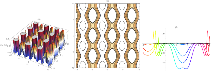
Semi-analytical wave solution of the Cahn–Allen equation by using Eq. (37) in three- (d), two- (f) dimensional, and contour (e) plots when \(x \in [-10,10]\), \(t \in [-10,10]\)
Figure 6 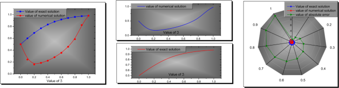
Numerical wave solution of the Cahn–Allen equation in combined, separated, and radar plots
- 2.
In Sect. 2.2, the Adomian decomposition method is applied to get the semi-analytical solutions, and by using one of the obtained analytical solution we explain the comparison between these solutions in Table 1.
Table 1 Comparison between analytical and semi-analytical solutions of the Cahn–Allen equation to calculate the values of absolute error, which explains the accuracy of both kinds of solutions - 3.
In Sect. 2.3, we apply the quintic B-spline to get the numerical solution of the Cahn–Allen equation. We explain the comparison between these solutions in Table 2.
Table 2 Comparison between analytical and numerical solutions of the Cahn–Allen equation to discuss the absolute error between both of them that explains the convergence between these solutions - 4.
According to Tables 1 and 2, we can see the superiority of the Adomian decomposition method on the quintic B-spline where the absolute error between the analytical and semi-analytical solutions is smaller than that obtained between analytical and numerical solutions.


4 Conclusion
In this paper, the modified auxiliary equation, the Adomian decomposition method, and the B-spline scheme were successfully implemented on the Cahn–Allen equation to get the analytical, semi-analytical, and numerical solutions that show the structure of the dynamics for phase separation in Fe–Cr–X (\(X=Mo, Cu\)) ternary alloys. Some solutions are sketched to represent and explain the physical properties of them. Moreover, the comparison between these distinct solutions is given in the tables to show the absolute error between exact, semi-analytical, and numerical solutions. These tables show the superiority of the Adomian decomposition method on the quintic B-spline, since the absolute error obtained by the first method is smaller than that obtained by the second method. The solutions were represented, allowing a physical interpretation and better interpretation of their properties. In summary, this paper studied the Cahn–Allen equation and found relevant solutions that provide new explanations of real-world industrial phenomena. As we see in our paper, some numerical schemes can also be applied to this equation, such as in [23–25], and studying and using these methods to our model will be our future work.
References
Fu, Q., Chen, M., Hu, S., McElroy, C.A., Mathijssen, R.H., Sparreboom, A., Baker, S.D.: Development and validation of an analytical method for regorafenib and its metabolites in mouse plasma. J. Chromatogr. B 1090, 43–51 (2018)
Karimi, K., Taherzadeh, M.J.: A critical review of analytical methods in pretreatment of lignocelluloses: composition, imaging, and crystallinity. Bioresour. Technol. 200, 1008–1018 (2016)
Barg, S., Flager, F., Fischer, M.: An analytical method to estimate the total installed cost of structural steel building frames during early design. J. Build. Eng. 15, 41–50 (2018)
Cieślik, B.M., Namieśnik, J., Konieczka, P.: Review of sewage sludge management: standards, regulations and analytical methods. J. Clean. Prod. 90, 1–15 (2015)
Lupoi, J.S., Singh, S., Parthasarathi, R., Simmons, B.A., Henry, R.J.: Recent innovations in analytical methods for the qualitative and quantitative assessment of lignin. Renew. Sustain. Energy Rev. 49, 871–906 (2015)
Sheikholeslami, M., Ganji, D.: Nanofluid convective heat transfer using semi analytical and numerical approaches: a review. J. Taiwan Inst. Chem. Eng. 65, 43–77 (2016)
Guan, X., Tang, J., Shi, D., Wang, Q., et al.: A semi-analytical method for transverse vibration of sector-like thin plate with simply supported radial edges. Appl. Math. Model. 60, 48–63 (2018)
Ebrahimi, F., Salari, E.: Size-dependent free flexural vibrational behavior of functionally graded nanobeams using semi-analytical differential transform method. Composites, Part B, Eng. 79, 156–169 (2015)
Wang, Q., Qin, B., Shi, D., Liang, Q.: A semi-analytical method for vibration analysis of functionally graded carbon nanotube reinforced composite doubly–curved panels and shells of revolution. Compos. Struct. 174, 87–109 (2017)
Bhatti, M.M., Abbas, M.A., Rashidi, M.M.: A robust numerical method for solving stagnation point flow over a permeable shrinking sheet under the influence of MHD. Appl. Math. Comput. 316, 381–389 (2018)
Solís-Pérez, J., Gómez-Aguilar, J., Atangana, A.: Novel numerical method for solving variable-order fractional differential equations with power, exponential and Mittag-Leffler laws. Chaos Solitons Fractals 114, 175–185 (2018)
Grylonakis, E.-N., Filelis-Papadopoulos, C.K., Gravvanis, G.A., Fokas, A.S.: An iterative spatial–stepping numerical method for linear elliptic PDEs using the Unified Transform. J. Comput. Appl. Math. 352, 194–209 (2019)
Haji, T.K., Marshall, A.M., Franza, A.: Mixed empirical–numerical method for investigating tunnelling effects on structures. Tunn. Undergr. Space Technol. 73, 92–104 (2018)
Chen, S., Liu, F., Turner, I., Anh, V.: A fast numerical method for two-dimensional Riesz space fractional diffusion equations on a convex bounded region. Appl. Numer. Math. 134, 66–80 (2018)
Lu, D., Seadawy, A.R., Khater, M.M.: Structures of exact and solitary optical solutions for the higher-order nonlinear Schrödinger equation and its applications in mono–mode optical fibers. Mod. Phys. Lett. B 33(23), 1950279 (2019)
Ali, A.T., Khater, M.M., Attia, R.A., Abdel-Aty, A.-H., Lu, D.: Abundant numerical and analytical solutions of the generalized formula of Hirota–Satsuma coupled KdV system. Chaos Solitons Fractals 109473 (2019)
Rezazadeh, H., Korkmaz, A., Khater, M.M., Eslami, M., Lu, D., Attia, R.A.: New exact traveling wave solutions of biological population model via the extended rational sinh–cosh method and the modified Khater method. Mod. Phys. Lett. A 33(28), 1950338 (2019)
Tang, Y., Tao, S., Guan, Q.: Lump solitons and the interaction phenomena of them for two classes of nonlinear evolution equations. Comput. Math. Appl. 72(9), 2334–2342 (2016)
Wazwaz, A.-M.: New \((3+ 1)\)-dimensional nonlinear evolution equations with Burgers and Sharma–Tasso–Olver equations constituting the main parts. Proc. Rom. Acad., Ser. A 16(1), 32–40 (2015)
Hajipour, M., Jajarmi, A., Baleanu, D., Sun, H.: On an accurate discretization of a variable-order fractional reaction–diffusion equation. Commun. Nonlinear Sci. Numer. Simul. 69, 119–133 (2019)
Khater, M.M.A., Baleanu, D.: On new analytical and semi-analytical wave solutions of the quadratic–cubic fractional nonlinear Schrödinger equation. Chaos, Interdiscip. J. Nonlinear Sci. (Submitted) (2019)
Khater, M.M.A., Baleanu, D.: On the new explicit computational and numerical solutions of the fractional nonlinear space–time Telegraph equation. Mod. Phys. Lett. A (Submitted) (2019)
Hajipour, M., Jajarmi, A., Baleanu, D.: On the accurate discretization of a highly nonlinear boundary value problem. Numer. Algorithms 79(3), 679–695 (2018)
Hajipour, M., Jajarmi, A., Malek, A., Baleanu, D.: Positivity-preserving sixth-order implicit finite difference weighted essentially non-oscillatory scheme for the nonlinear heat equation. Appl. Math. Comput. 325, 146–158 (2018)
Kumar, D., Singh, J., Tanwar, K., Baleanu, D.: A new fractional exothermic reactions model having constant heat source in porous media with power, exponential and Mittag-Leffler laws. Int. J. Heat Mass Transf. 138, 1222–1227 (2019)
Singh, J., Kumar, D., Baleanu, D.: On the analysis of fractional diabetes model with exponential law. Adv. Differ. Equ. 2018(1), 231 (2018)
Kumar, D., Singh, J., Baleanu, D.: A new analysis of the Fornberg–Whitham equation pertaining to a fractional derivative with Mittag-Leffler-type kernel. Eur. Phys. J. Plus 133(2), 70 (2018)
Kumar, D., Singh, J., Purohit, S.D., Swroop, R.: A hybrid analytical algorithm for nonlinear fractional wave–like equations. Math. Model. Nat. Phenom. 14(3), 304 (2019)
Kumar, D., Tchier, F., Singh, J., Baleanu, D.: An efficient computational technique for fractal vehicular traffic flow. Entropy 20(4), 259 (2018)
Goswami, A., Singh, J., Kumar, D., et al.: An efficient analytical approach for fractional equal width equations describing hydro–magnetic waves in cold plasma. Phys. A, Stat. Mech. Appl. 524, 563–575 (2019)
Khater, M., Attia, R.A., Lu, D.: Explicit Lump Solitary Wave of Certain Interesting \((3+ 1)\)-Dimensional Waves in Physics via Some Recent Traveling Wave Methods. Entropy 21(4), 397 (2019)
Khater, M.M., Lu, D., Attia, R.A.: Dispersive long wave of nonlinear fractional Wu–Zhang system via a modified auxiliary equation method. AIP Adv. 9(2), 025003 (2019)
Khater, M.M., Lu, D., Attia, R.A.: Lump soliton wave solutions for the \((2+ 1)\)-dimensional Konopelchenko–Dubrovsky equation and KdV equation. Mod. Phys. Lett. B 33, 1950199 (2019)
Attia, R.A., Lu, D., Khater, M.M.A.: Chaos and relativistic energy–momentum of the nonlinear time fractional Duffing equation. Math. Comput. Appl. 24(1), 10 (2019)
Khater, M., Attia, R., Lu, D.: Modified Auxiliary Equation Method versus Three Nonlinear Fractional Biological Models in Present Explicit Wave Solutions. Math. Comput. Appl. 24(1), 1 (2019)
Prakash, A., Kaur, H.: Analysis and numerical simulation of fractional order Cahn–Allen model with Atangana–Baleanu derivative. Chaos Solitons Fractals 124, 134–142 (2019)
Hosseini, K., Bekir, A., Ansari, R.: New exact solutions of the conformable time-fractional Cahn–Allen and Cahn–Hilliard equations using the modified Kudryashov method. Optik 132, 203–209 (2017)
Bulut, H., Atas, S.S., Baskonus, H.M.: Some novel exponential function structures to the Cahn–Allen equation. Cogent Phys. 3(1), 1240886 (2016)
Ji, B., Liao, H.-l., Zhang, L.: Simple maximum–principle preserving time-stepping methods for time-fractional Allen–Cahn equation (2019). arXiv:1906.11693. Preprint
Acknowledgements
Mostafa Khater would like to dedicate this paper to his mother, son (Adam) and the soul of his father; their love, support, and constant care will never be forgotten.
Availability of data and materials
Not applicable.
Funding
Not applicable.
Author information
Authors and Affiliations
Contributions
All authors conceived of the study, participated in its design and coordination, drafted the manuscript, participated in the sequence alignment, and read and approved the final manuscript.
Corresponding author
Ethics declarations
Competing interests
The authors declare that they have no competing interests.
Additional information
Publisher’s Note
Springer Nature remains neutral with regard to jurisdictional claims in published maps and institutional affiliations.
Rights and permissions
Open Access This article is licensed under a Creative Commons Attribution 4.0 International License, which permits use, sharing, adaptation, distribution and reproduction in any medium or format, as long as you give appropriate credit to the original author(s) and the source, provide a link to the Creative Commons licence, and indicate if changes were made. The images or other third party material in this article are included in the article’s Creative Commons licence, unless indicated otherwise in a credit line to the material. If material is not included in the article’s Creative Commons licence and your intended use is not permitted by statutory regulation or exceeds the permitted use, you will need to obtain permission directly from the copyright holder. To view a copy of this licence, visit http://creativecommons.org/licenses/by/4.0/.
About this article

Cite this article
Khater, M.M.A., Park, C., Lu, D. et al. Analytical, semi-analytical, and numerical solutions for the Cahn–Allen equation. Adv Differ Equ 2020, 9 (2020). https://doi.org/10.1186/s13662-019-2475-8
Received:
Accepted:
Published:
DOI: https://doi.org/10.1186/s13662-019-2475-8