Family of odd point non-stationary subdivision schemes and their applications

Abstract

The $(2s-1)$-point non-stationary binary subdivision schemes (SSs) for curve design are introduced for any integer $s\geq 2$. The Lagrange polynomials are used to construct a new family of schemes that can reproduce polynomials of degree $(2s-2)$. The usefulness of the schemes is illustrated in the examples. Moreover, the new schemes are the non-stationary counterparts of the stationary schemes of (Daniel and Shunmugaraj in 3rd International Conference on Geometric Modeling and Imaging, pp. 3–8, 2008; Hassan and Dodgson in Curve and Surface Fitting: Sant-Malo 2002, pp. 199–208, 2003; Hormann and Sabin in Comput. Aided Geom. Des. 25:41–52, 2008; Mustafa et al. in Lobachevskii J. Math. 30(2):138–145, 2009; Siddiqi and Ahmad in Appl. Math. Lett. 20:707–711, 2007; Siddiqi and Rehan in Appl. Math. Comput. 216:970–982, 2010; Siddiqi and Rehan in Eur. J. Sci. Res. 32(4):553–561, 2009). Furthermore, it is concluded that the basic shapes in terms of limiting curves produced by the proposed schemes with fewer initial control points have less tendency to depart from their tangent as well as their osculating plane compared to the limiting curves produced by existing non-stationary subdivision schemes.

1 Introduction

The importance of SSs cannot be denied because they play a vital role in computer-aided geometric designing (CAGD), geometric modeling, computer graphics, medical image processing, scientific visualization, reverse engineering, robotics, etc. Nowadays, SSs can be distinguished in various types: they can range from uniform to non-uniform; from binary to an arbitrary arity; from interpolatory to approximating; from stationary to non-stationary. It seems that stationary SSs have interesting features, but reconstruction of special types of limit curves of various shapes, including polynomial functions, conic sections such as circles, ellipses, and spiral curves, could not be accomplished without the non-stationary SSs.

In literature, several articles have been published during the last couple of decades. In 2003, Jena et al. [13] constructed a 4-point interpolating non-stationary SS generating limit curves of $C^{1}$-continuity. In 2007, Beccari et al. [2] derived a non-stationary binary 4-point uniform tension controlled interpolating SS reproducing conics, and they also proposed another ternary 4-point $C^{2}$-continuous interpolating non-stationary SS with tension control [3] in the same year. In 2009, Daniel and Shunmugaraj [6] introduced a 6-point binary interpolating non-stationary SS that is $C^{2}$ limit curve. Conti and Romani [4] presented and investigated a 6-point interpolatory non-stationary subdivision SS capable of reproducing important curves in 2010. In 2007, Daniel and Shunmugaraj [7] introduced some 4-point ternary interpolating non-stationary schemes. In 2013, Li et al. [16] developed a new technique to establish a non-stationary SS that can generate functions in a finite-dimensional subspace of exponential polynomials. Mustafa et al. [19] introduced a subdivision-regularization framework for preventing over-fitting of data by a model in 2013. In 2016, Salam et al. [23] presented two non-stationary forms of Chaikin perturbation SS, and Tan et al. [27] derived a 3-point approximating non-stationary SS. For more recent work on SSs, one may be referred to [1, 15, 17, 18, 21].

Another aim of this research is to discuss and compare the limit curves of our proposed SSs. Also, we have measured curvature and torsion to find the rate at which limiting curves approach to deviate from their tangents. It is observed that the limit curves of our approximating schemes are near to the initial control polygons and for a certain range of parameter limit curves pass through the initial polygons. Moreover, the proposed SSs are non-stationary counterparts of the stationary SSs of [5, 11, 12, 22, 24,25,26].

The plan of this article is as follows: Sect. 2 is devoted to the introduction of some basic identities and definitions. We also derived some lemmas that are applied for construction of $(2 s-1)$-point non-stationary. Construction and smoothness of the proposed SSs are discussed in Sect. 3. Section 4 deals with various properties such as the shape of the limit curve, curvature, and torsion, while Sect. 5 is concerned with the conclusion.

2 Preliminaries and definition

A general form of univariate binary subdivision scheme S which maps a polygon $\alpha ^{j}=\{\alpha ^{j}_{i}\}_{i\in \mathbb{Z}}$ to a refined polygon $\alpha ^{j+1}=\{\alpha ^{j+1}_{i}\}_{i\in \mathbb{Z}}$ is defined by

$$ q_{2i+\gamma }^{j+1}=\sum^{s}_{k=0} \alpha _{i+\gamma }^{j}q_{i+k}^{j},\quad \gamma =0,1, $$

(1)

where $s > 0$, $\mathbb{Z}$ is the set of integers. The set of coefficients $\{\alpha ^{j}_{i,\gamma }, \gamma =0,1\}_{k=0}^{s}$ is called subdivision mask. This scheme is formally denoted by $q^{j+1}=Sq^{j}$.

A necessary condition for uniform convergence of the subdivision scheme (1) is

$$ \sum^{s}_{k=0} \alpha ^{j}_{i,\gamma } \cong 1, \quad \gamma =0,1. $$

(2)

For the given s, we define Lagrange fundamental polynomials of degree $2s-2$ and $2s-3$ corresponding to nodes $\{t\}^{s-1}_{-(s-1)}$ and $\{t\}^{s-2}_{-(s-1)}$, respectively, and they are

$$ L_{t}^{2s-2}(x)=\prod _{j=-(s-1),t\neq j}^{s-1} \frac{(x-j)}{(t-j)}, $$

(3)

where $t= -(s-1),-(s-2),\ldots ,(s-1)$, and

$$ L_{t}^{2s-3}(x)=\prod _{j=-(s-2),t\neq j}^{s-1} \frac{(x-j)}{(t-j)}, $$

(4)

where $t=-(s-2),-(s-3),\ldots ,(s-1)$.

Lemma 1

([20])

If $t=-(s-1),\ldots,(s-1)$, then the following implication holds:

$$ \prod_{j=-(s-1), j\neq t}^{s-1}(t-j)=(-1)^{s-t-1}(s+t-1)!(s-t-1)!. $$

(5)

Lemma 2

([20])

If $t=-(s-2),\ldots ,(s-1)$, then following implication holds:

$$ \prod_{j=-(s-2), j\neq t}^{s-1}(t-j)=(-1)^{s-t-1}(s+t-2)!(s-t-1)!. $$

(6)

Lemma 3

([20])

If $L^{2s-2}_{t} (x )$ is a Lagrange fundamental polynomial of degree $(2s-2)$ corresponding to nodes $\{t\}^{s-1}_{-(s-1)}$ defined by (3), then

$$ L^{2s-2}_{t} \biggl(\frac{1}{4} \biggr)= \frac{(-1)^{t}(4s-3)!}{2^{6s-6}(2s-2)!(1-4t)(s-t-1)!(s+t-1)!}, $$

(7)

where $t= -(s-1), \ldots , (s-1)$.

Lemma 4

([20])

If $L^{2s-3}_{t}(x)$ is a Lagrange fundamental polynomial of degree $(2s-3)$ defined by (4) corresponding to the nodes $\{t\}^{s-1}_{-(s-2)}$, then we get

$$ L^{2s-3}_{t} \biggl(\frac{1}{4} \biggr)= \frac{(-1)^{t}(4s-5)(4s-7)!}{2^{6s-10}(1-4t)(2s-4)!(s+t-2)!(s-t-1)!}, $$

(8)

where $t=-(s-2),\ldots,(s-1)$.

Lemma 5

If $t=-(s-2),\ldots ,(s-1)$, then the following implication holds:

$$\begin{aligned} \beta _{t}^{k} =& \frac{\sin (\frac{\theta }{2^{k+1}} (\prod_{ {j=-(s-2)},{j\neq t}}^{s-1} (\frac{1}{4}-j ) ) )}{ \sin (\frac{\theta }{2^{k+1}} (\prod_{j=-(s-2), j\neq t} ^{s-1}(t-j) ) )} \\ =&\frac{\sin (\frac{\theta }{2^{k+1}} (\frac{(-1)^{s-1}(4s-5)(4s-7)!}{2^{6s-10}(2s-4)!(1-4t)} ) )}{ \sin (\frac{\theta }{2^{k+1}} ( -1 ) ^{s-t-1} ((s-t-1)!(s+t-2)! ) )}. \end{aligned}$$

(9)

Proof

Since

$$\begin{aligned} \prod_{j=-(s-2)}^{s-1} \biggl(\frac{1}{4}-j \biggr) =& \biggl(\frac{1}{4} \biggr) ^{2s-2} \bigl\{ (4s-7) (4s-11) \cdots (5) (1) (-3)\cdots (-4s+13) \\ &{}\times (-4s+9) (-4s+5)\bigr\} , \end{aligned}$$

then

$$ \prod_{j=-(s-2), j\neq t}^{s-1} \biggl(\frac{1}{4}-j \biggr)= \frac{1}{4^{2s-3}(1-4t)}\prod_{t=-s+2}^{s-1} (1-4t ). $$

This implies

$$\begin{aligned} \prod_{j=-(s-2), j\neq t}^{s-1} \biggl(\frac{1}{4}-j \biggr) =& \frac{(-1)^{s-1}}{4^{2s-3}(1-4t)}\biggl\{ (4s-7) \\ &{}\times \frac{(4s-8)}{(4s-8)} \frac{(4s-9)}{(4s-9)} \frac{(4s-10)}{(4s-10)} (4n-11) \\ &{}\times \frac{(4s-12)}{(4s-12)}\cdots \biggl(\frac{8}{8} \biggr) \biggl( \frac{7}{7} \biggr) \biggl(\frac{6}{6} \biggr) (5 ) \biggl( \frac{4}{4} \biggr) \biggl(\frac{3}{3} \biggr) \\ &{}\times \biggl(\frac{2}{2} \biggr) (1 ) \biggl(\frac{2}{2} \biggr) (3) \biggl(\frac{4}{4} \biggr) \biggl(\frac{5}{5} \biggr) \biggl(\frac{6}{6} \biggr) (7) \cdots (4s-13) \\ &{}\times \frac{(4s-12)}{(4s-12)}\frac{(4s-11)}{(4s-11)} \frac{(4s-10)}{(4s-10)}(4s-9) \\ &{}\times \frac{(4s-8)}{(4s-8)}\frac{(4s-7)}{(4s-7)} \frac{(4s-6)}{(4s-6)} (4s-5) \frac{(4s-4)}{(4s-4)}\biggr\} . \end{aligned}$$

This leads to

$$ \prod_{{j=-(s-2)},{j\neq t}}^{s-1} \biggl( \frac{1}{4}-j \biggr)= \frac{(-1)^{s-1}(4s-5)(4s-7)!}{2^{6s-10}(1-4t)(2s-4)!}. $$

(10)

Using (6) and (10), we get (9). This completes the proof. □

Theorem 6

If $L^{2s-2}_{t}(x)$ and $L^{2s-3}_{t}(x)$ are Lagrange fundamental polynomials of degree $(2s-2)$ and $(2s-3)$ corresponding to the nodes $\{t\}^{s-1}_{-(s-1)}$ and $\{t\}^{s-1}_{-(s-2)}$, respectively, then the following implication holds:

$$\begin{aligned} \lambda _{t}^{k} =&\frac{\sin (\frac{\theta }{2^{k+1}} (L _{t}^{2s-2}(\frac{1}{4})-L_{t}^{2s-3}(\frac{1}{4}) ) )}{ \sin (\frac{\theta }{2^{k+1}} (L_{-s+1}^{2s-2}(\frac{1}{4}) ) )} \\ =&\frac{\sin (\frac{\theta }{2^{k+1}} (\frac{(-1)^{t}(4s-4)!}{2^{6s-6}(2s-2)!(s-t-1)!(s+t-1)!} ) )}{ \sin (\frac{\theta }{2^{k+1}} (\frac{(-1)^{-s+1}(4s-3)!}{2^{6s-6}(4s-3)(2s-2)!(2s-2)!} ) )}, \end{aligned}$$

(11)

where $t=-(s-2),\ldots ,(s-1)$.

Proof

Since

$$ L_{t}^{2s-2} \biggl(\frac{1}{4} \biggr)-L_{t}^{2s-3} \biggl(\frac{1}{4} \biggr) = \frac{(-1)^{t}(4s-4)!}{2^{6s-6}(2s-2)!(s-t-1)!(s+n-1)!} $$

(12)

and substituting $t=-(s-1)$ in (7), we have

$$ L_{-(s-1)}^{2s-2} \biggl(\frac{1}{4} \biggr)= \frac{(-1)^{-s+1}(4s-3)!}{2^{6s-6}(4s-3)(2s-2)!(2s-2)!}. $$

(13)

Using (12) and (13), we get (11), which completes the proof. □

3 The $(2 s-1)$-point non-stationary SS

In this section, we present general explicit formulae to construct the mask of a $(2s-1)$-point non-stationary binary approximating subdivision scheme.

Now, for $s\geq 2$, the mask of $(2s-1)$-point binary approximating schemes SS can be generated by

$$ \textstyle\begin{cases} p_{2i}^{k+1}=\sum_{t=-(s-1)}^{s-1} \eta _{-t}^{k} p_{i+t} ^{k}, \\ p_{2i+1}^{k+1}=\sum_{t=-(s-1)}^{s-1} \eta _{t}^{k} p_{i+t} ^{k}, \end{cases} $$

(14)

can be generated by

$$ \textstyle\begin{cases} \eta _{-s+1}^{k}= \frac{\sin (\frac{\theta \mu }{2^{k+1}} )}{ \sin (\frac{\theta }{2^{k+1}} )}, \quad \mu < 1, \\ \eta _{t}^{k}=\beta _{t}^{k}+\lambda _{t}^{k}\mu , \quad t=-s+2,\ldots,s-1, \end{cases} $$

(15)

where

$$\begin{aligned}& \beta _{t}^{k} =\frac{\sin (\frac{\theta }{2^{k+1}} \frac{(-1)^{s-1}(4s-5)(4s-7)!}{2^{6s-10}(1-4t)(2s-4)!} )}{ \sin (\frac{\theta }{2^{k+1}}(-1)^{s-t-1}(s-t-1)!(s+t-2)! )}, \\& \lambda _{m}^{k} =\frac{\sin (\frac{\theta }{2^{k+1}} \frac{(-1)^{t}(4s-4)!}{2^{6s-6}(2s-2)!(s-t-1)!(s+t-1)!} )}{ \sin (\frac{\theta }{2^{k+1}} \frac{(-1)^{-s+1}(4s-4)!}{2^{6s-4}((2s-2)!)^{2}} )}, \end{aligned}$$

and μ and θ are free parameters.

Here we see that some of the schemes are special cases of the scheme proposed above. Some of new non-stationary schemes are also given below.

• Substituting $s=2$ in (14) and (15), we get a new 3-point symmetric binary approximating SS with free parameters μ and θ:

  $$ \begin{aligned} &p^{k+1}_{2i} =\eta _{1}^{k}p^{k}_{i-1}+\eta _{0}^{k}p^{k}_{i} +\eta _{-1}^{k}p^{k}_{i+1}, \\ &p^{k+1}_{2i+1} =\eta _{-1}^{k}p^{k}_{i-1}+ \eta _{0}^{k}p^{k}_{i} +\eta _{1}^{k}p^{k}_{i+1}, \end{aligned} $$

  (16)

  where

  $$\begin{aligned}& \eta _{-1}^{k}=\frac{\sin (\frac{\theta \mu }{2^{k+1}} )}{ \sin (\frac{\theta }{2^{k+1}} )}, \\& \eta _{0}^{k}=\frac{\sin (\frac{1}{4}\frac{3\theta }{2^{k+1}} )}{ \sin (\frac{\theta }{2^{k+1}} )}-\frac{\sin (\frac{1}{16}\frac{3 \theta }{2^{k+1}} )}{\sin (\frac{1}{32} \frac{3\theta }{2^{k+1}} )}\mu , \\& \eta _{1}^{k}=\frac{\sin (\frac{1}{4}\frac{\theta }{2^{k+1}} )}{ \sin (\frac{\theta }{2^{k+1}} )}+ \mu . \end{aligned}$$

• Substituting $s=3$ in (14) and (15), we get a new 5-point symmetric binary approximating SS with free parameters μ and θ:

  $$ \begin{aligned} &p^{k+1}_{2i}=\eta _{2}^{k}p^{k}_{i-2}+\eta _{1}^{k}p^{k}_{i-1}+\eta _{0} ^{k}p^{k}_{i} +\eta _{-1}^{k}p^{k}_{i+1}+ \eta _{-2}^{k}p^{k}_{i+2}, \\ &p^{k+1}_{2i+1}=\eta _{-2}^{k}p^{k}_{i-2}+ \eta _{-1}^{k}p^{k}_{i-1}+\eta _{0}^{k}p^{k}_{i} +\eta _{1}^{k}p^{k}_{i+1}+\eta _{2}^{k}p^{k}_{i+2}, \end{aligned} $$

  (17)

  where

  $$\begin{aligned}& \eta _{-2}^{k}=\frac{\sin (\frac{\theta \mu }{2^{k+1}} )}{ \sin (\frac{\theta }{2^{k+1}} )}, \\& \eta _{-1}^{k}=-\frac{\sin (\frac{1}{64} \frac{21\theta }{2^{k+1}} )}{\sin (\frac{6\theta }{2^{k+1}} )}- \frac{\sin (\frac{1}{512}\frac{35\theta }{2^{k+1}} )}{ \sin (\frac{1}{2048}\frac{35\theta }{2^{k+1}} )}\mu , \\& \eta _{0}^{k}=\frac{\sin (\frac{1}{64} \frac{105\theta }{2^{k+1}} )}{\sin (\frac{2\theta }{2^{k+1}} )}+ \frac{\sin (\frac{1}{1024}\frac{105\theta }{2^{k+1}} )}{ \sin (\frac{1}{2048}\frac{35\theta }{2^{k+1}} )}\mu , \\& \eta _{1}^{k}=\frac{\sin (\frac{1}{64} \frac{35\theta }{2^{k+1}} )}{\sin (\frac{2\theta }{2^{k+1}} )}- \frac{\sin (\frac{1}{512}\frac{35\theta }{2^{k+1}} )}{ \sin (\frac{1}{2048}\frac{35\theta }{2^{k+1}} )}\mu , \\& \eta _{2}^{k}=-\frac{\sin (\frac{1}{64} \frac{15\theta }{2^{k+1}} )}{\sin (\frac{6\theta }{2^{k+1}} )}+ \mu . \end{aligned}$$

3.1 Convergence and smoothness of the proposed SS

In this section, we use asymptotic equivalence method to find the smoothness of the normalized SSs (16) and (17).

Definition 1

Two binary SSs $\{S_{\alpha _{j}}\}$ and $\{S_{\beta _{j}}\}$ are asymptotically equivalent if

$$ \sum^{\infty }_{j=1}\Vert S_{\alpha _{j}} - S_{\beta _{j}} \Vert < \infty , $$

where $\Vert S_{\alpha _{j}} \Vert _{\infty } =\max \{ \sum_{i\in \mathbb{Z}}\vert \alpha ^{(j)}_{2i}\vert , \vert \alpha ^{(j)}_{2i+1}\vert \}$.

Theorem 7

([9])

Consider $\{S_{\alpha _{j}}\}$ is a non-stationary SS and $\{S_{\beta _{j}}\}$ is a stationary SS. Let $\{S_{\alpha _{j}}\}$ and $\{S_{\beta _{j}}\}$ be the two asymptotically equivalent SSs having finite masks of the same support. If $\{S_{\beta _{j}}\}$ is $C^{m}$ and $\sum^{ \infty }_{j=0}2^{mj}\Vert S_{\alpha _{j}} - S_{\beta _{j}} \Vert < \infty$, then the non-stationary SS $\{S_{a_{j}}\}$ is $C^{m}$.

Some estimates of stencils $\eta ^{j}_{i}$, $i=0,1$, and $\lambda ^{j} _{i}$, $i=-1,0,1,2$, are required to find smoothness of the proposed schemes which are given in the following lemmas.

Lemma 8

For some $k\geq 0$ and $0<\theta <\frac{\pi }{2}$,

$$\begin{aligned} (\mathrm{a})&\quad \mu \leq \eta _{-1}^{k}\leq \frac{\mu }{\cos (\frac{ \theta }{2^{k+1}} )}; \\ (\mathrm{b})&\quad \biggl(\frac{3}{4}-2\mu \biggr)\leq \eta _{0}^{k}\leq \biggl(\frac{3}{4 \cos (\frac{\theta }{2^{k+1}} )} -2\cos \biggl( \frac{1}{32}\frac{3 \theta }{2^{k+1}} \biggr)\mu \biggr); \\ (\mathrm{c})&\quad \biggl(\frac{1}{4}+\mu \biggr)\leq \eta _{1}^{k}\leq \biggl(\frac{1}{4 \cos (\frac{\theta }{2^{k+1}} )}+\mu \biggr). \end{aligned}$$

Proof

We give the proof of (a). Note that

$$ \eta _{-1}^{k}= \frac{\sin (\frac{\theta \mu }{2^{k+1}} )}{ \sin (\frac{\theta }{2^{k+1}} )}\geq \frac{\frac{\theta \mu }{2^{k+1}}}{\frac{\theta }{2^{k+1}}}= \mu $$

and

$$ \eta _{-1}^{k}\leq \frac{\sin (\frac{\theta \mu }{2^{k+1}} )}{ \sin (\frac{\theta }{2^{k+1}} ) } \leq { \frac{\frac{ \theta \mu }{2^{k+1}}}{\frac{\theta }{2^{k+1}}\cos ( {\frac{ \theta }{2^{k+1}}} )}} \leq \frac{\mu }{\cos (\frac{ \theta }{2^{k+1}} )}. $$

This completes the proof of (a) the proofs of (b) and (c) are obtained in a similar way. □

By Lemma 8, we get the following lemma.

Lemma 9

$$\begin{aligned} (\mathrm{a})&\quad \bigl\vert \eta _{-1}^{k}-\mu \bigr\vert \leq C_{0} \frac{1}{2^{3k}}, \\ (\mathrm{b})&\quad \biggl\vert \eta _{0}^{k}- \biggl( \frac{3}{4}-2\mu \biggr) \biggr\vert \leq C_{1} \frac{1}{2^{3k}}, \\ (\mathrm{c})&\quad \biggl\vert \eta _{1}^{k}- \biggl( \frac{1}{4}+\mu \biggr) \biggr\vert \leq C_{2} \frac{1}{2^{3k}}, \end{aligned}$$

where $C_{0}$, $C_{1}$, and $C_{2}$ are some constants independent of k.

Proof

We give the proof of (a). By (a) of Lemma 8, we have

$$\begin{aligned} \bigl\vert \eta _{-1}^{k}-\mu \bigr\vert \leq &\mu \biggl(\frac{1-\cos (\frac{ \theta }{2^{k+1}} )}{\cos (\frac{\theta }{2^{k+1}} )} \biggr) \\ \leq &\frac{2\mu }{\cos (\frac{\theta }{2^{k+1}} )}\sin ^{2} \biggl(\frac{\theta }{2^{k+2}} \biggr) \\ \leq &\frac{2\mu \theta ^{2}}{16\cos (\theta )} \frac{1}{2^{3k}}\leq C_{0} \frac{1}{2^{3k}}. \end{aligned}$$

This proves (a). The proofs of (b) and (c) are similar. □

Remark 1

The proposed 3-point SS (16) is a non-stationary counterpart of the following stationary SS:

$$ \textstyle\begin{cases} p^{k+1}_{2i}= (\frac{1}{4}+\mu )p^{k}_{i-1}+ (\frac{3}{4}-2 \mu )p^{k}_{i}+\mu p^{k}_{i+1}, \\ p^{k+1}_{2i+1}=\mu p^{k}_{i-1}+ (\frac{3}{4}-2\mu )p^{k} _{i}+ (\frac{1}{4}+\mu )p^{k}_{i+1}, \end{cases} $$

(18)

as the stencils of the normalized SS (16) converge to the stencils of (18): $\eta _{-1}^{k}\rightarrow \mu$, $\eta _{0}^{k}\rightarrow (\frac{3}{4}-2\mu )$, and $\eta _{1}^{k}\rightarrow (\frac{1}{4}+\mu )$ as $k\rightarrow \infty$. The proofs of these convergences follow from Lemma 9.

Remark 2

Similarly, for $n=2$ and $\mu =-3\omega$, $\mu =\frac{1}{16}$, $\mu =\frac{-3}{32}$, $\mu =\frac{1}{24}+\frac{1}{4}w$, $\mu = \frac{1}{32}$, and $\mu =\frac{-3}{32}+w$, in (14) and (15), we get non-stationary counterparts of the stationary 3-point schemes of [5, 11, 12, 22, 24, 26] respectively.

Lemma 10

The Laurent polynomial $\alpha (z)$ of scheme (18) can be written as

$$\begin{aligned} \alpha (z) =&\biggl\{ \mu + \biggl(\frac{1}{4}+\mu \biggr)z+ \biggl( \frac{3}{4}-2 \mu \biggr)z^{2} + \biggl(\frac{3}{4}-2\mu \biggr)z^{3} \\ &{}+ \biggl(\frac{1}{4}+\mu \biggr)z^{4}+\mu z^{5} \biggr\} , \end{aligned}$$

and a subdivision scheme $S_{\alpha }$ corresponding to the symbol $\alpha (z)$is $C^{2}$ for $\mu \in (0,\frac{1}{8} )$ and $C^{3}$ for $\mu =\frac{1}{16}$.

Proof

Consider

$$ c(z)=\frac{8 \alpha (z)}{(1+z)^{3}}= \bigl(8\mu +(2-16\mu )z+8\mu z ^{2} \bigr). $$

Note that, for $\mu \in (0,\frac{1}{8} )$,

$$\begin{aligned} \biggl\Vert \frac{1}{2}S_{c} \biggr\Vert =& \frac{1}{2}\max \biggl\{ \sum_{j \in \mathbb{Z}} \vert c_{2j} \vert ,\sum_{j \in \mathbb{Z}} \vert c _{2j+1} \vert \biggr\} \\ =&\frac{1}{2}\max \bigl\{ 2 \vert 8\mu \vert , \vert 2-16 \mu \vert \bigr\} < 1. \end{aligned}$$

So the scheme is $C^{2}$-continuous for $\mu \in (0,\frac{1}{8} )$. In order to prove $C^{3}$ smoothness, we put $\mu =\frac{1}{16}$ in $c(z)$, that is,

$$ c(z)=\frac{1}{2} \bigl(1+2z+z^{2} \bigr). $$

If

$$ d(z)=\frac{2c(z)}{(1+z)}= (1+z ), $$

then $\Vert \frac{1}{2}S_{d} \Vert =\frac{1}{2}\max \{\sum_{j \in \mathbb{Z}} \vert d_{2j} \vert ,\sum_{j \in \mathbb{Z}} \vert d _{2j+1} \vert \}=\max \{\frac{1}{2},\frac{1}{2} \}<1$. Hence by ([10], Corollary 4.11) the stationary SS $S_{\alpha }$ is $C^{3}$. □

Theorem 11

The stationary SSs (16) and (18) are asymptotically equivalent, that is,

$$ \sum_{k=0}^{\infty } \Vert S_{\alpha ^{k}}-S_{\alpha } \Vert _{ \infty }< \infty . $$

Proof

From (16) and (18), we have

$$\begin{aligned} \sum_{k=0}^{\infty }\|S_{\alpha ^{k}}-S_{\alpha } \|_{\infty } =&\sum_{k=0}^{\infty }\biggl\{ \bigl\vert \eta _{-1}^{k}-\mu \bigr\vert + \biggl\vert \eta _{0}^{k}- \biggl(\frac{3}{4}-2\mu \biggr) \biggr\vert \\ &{}+ \biggl\vert \eta _{1}^{k}- \biggl( \frac{1}{4}+\mu \biggr) \biggr\vert \biggr\} . \end{aligned}$$

From (a) of Lemma 9, it follows that

$$ \sum_{k=0}^{\infty } \bigl\vert \eta _{-1}^{k}-\mu \bigr\vert \leq \sum _{k=0}^{\infty }C _{0}\frac{1}{2^{3k}}< \infty . $$

Similarly, from (a) and (b) of Lemma 9, we have

$$ \sum_{k=0}^{\infty } \biggl\vert \eta _{0}^{k}- \biggl(\frac{3}{4}-2\mu \biggr) \biggr\vert < \infty , \qquad \sum_{k=0}^{\infty } \biggl\vert \eta _{1}^{k}- \biggl(\frac{1}{4}+ \mu \biggr) \biggr\vert < \infty . $$

Hence

$$ \sum_{k=0}^{\infty } \Vert S_{\alpha ^{k}}-S_{\alpha } \Vert _{ \infty }< \infty . $$

 □

Theorem 12

The non-stationary SS (16) is $C^{2}$ for $\mu \in (0, \frac{1}{8} )$ and $C^{3}$ for $\mu =\frac{1}{16}$.

Proof

Since $S_{\alpha }$ is $C^{3}$ by Lemma 10 and also SSs (17) and (18) are asymptotically equivalent by Theorem 11, now by ([10], Theorem 8(a)), it is sufficient to prove that

$$ \sum_{k=0}^{\infty }2^{3k} \Vert S_{\alpha ^{k}}-S_{\alpha } \Vert _{\infty }< \infty , $$

where

$$\begin{aligned} \|S_{\alpha ^{k}}-S_{\alpha }\|_{\infty } =& \max \biggl\{ \sum _{j\in \mathbb{Z}} \bigl\vert \alpha _{2j}^{k}- \alpha _{2j} \bigr\vert , \sum_{j\in \mathbb{Z}} \bigl\vert \alpha _{2j+1}^{k}-\alpha _{2j+1} \bigr\vert \biggr\} \\ =& \bigl\vert \eta _{-1}^{k}-\mu \bigr\vert + \biggl\vert \eta _{0}^{k}- \biggl(\frac{3}{4}-2 \mu \biggr) \biggr\vert + \biggl\vert \eta _{1}^{k}- \biggl( \frac{1}{4}+\mu \biggr) \biggr\vert . \end{aligned}$$

This implies

$$\begin{aligned} \sum_{k=0}^{\infty }2^{3k} \|S_{\alpha ^{k}}-S_{\alpha }\|_{\infty } =& \sum _{k=0}^{\infty }2^{3k} \bigl\vert \eta _{-1}^{k}-\mu \bigr\vert \\ &{}+\sum_{k=0}^{\infty }2^{3k} \biggl\vert \eta _{0}^{k}- \biggl(\frac{3}{4}-2 \mu \biggr) \biggr\vert \\ &{}+\sum_{k=0}^{\infty }2^{3k} \biggl\vert \eta _{1}^{k}- \biggl(\frac{1}{4}+ \mu \biggr) \biggr\vert . \end{aligned}$$

Since by (a), (b), and (c) of Lemma 9, we have

$$ \sum_{k=0}^{\infty }2^{3k} \bigl\vert \eta _{-1}^{k}-\mu \bigr\vert < \infty ,\qquad \sum _{k=0}^{\infty }2^{3k} \biggl\vert \eta _{0}^{k}- \biggl(\frac{3}{4}-2 \mu \biggr) \biggr\vert < \infty $$

and

$$ \sum_{k=0}^{\infty }2^{3k} \biggl\vert \eta _{1}^{k}- \biggl(\frac{1}{4}+ \mu \biggr) \biggr\vert < \infty , $$

it follows that

$$ \sum_{k=0}^{\infty }2^{3k} \Vert S_{\alpha ^{k}}-S_{\alpha } \Vert _{\infty }< \infty . $$

 □

Here we will discuss the convergence and smoothness of 5-point SS (17). The proofs of lemmas given below are similar to the proofs of Lemmas 8 and 9.

Lemma 13

For some $k\geq 0$ and $0<\theta <\frac{\pi }{2}$,

$$\begin{aligned} (\mathrm{a}) &\quad \mu \leq \eta _{-2}^{k}\leq \frac{\mu }{\cos (\frac{ \theta }{2^{k+1}} )}; \\ (\mathrm{b}) &\quad {-}\frac{7}{128\cos (\frac{6\theta }{2^{k+1}} )} -\frac{4 \mu }{\cos (\frac{1}{2048}\frac{35\theta }{2^{k+1}} )} \leq \eta _{-1}^{k}\leq -\frac{7}{128}-4\mu ; \\ (\mathrm{c}) &\quad \frac{105}{128}+6\mu \leq \eta _{0}^{k} \leq \frac{105}{128 \cos (\frac{2\theta }{2^{k+1}} )} +\frac{6\mu }{\cos (\frac{1}{2048}\frac{35\theta }{2^{k+1}} )}; \\ (\mathrm{d}) &\quad \frac{35}{128}-4\mu \leq \eta _{1}^{k} \leq \frac{105}{128}-4 \mu \cos \biggl(\frac{1}{512}\frac{35\theta }{2^{k+1}} \biggr); \\ (\mathrm{e}) &\quad {-}\frac{5}{128\cos (\frac{6\theta }{2^{k+1}} )}+ \mu \leq \eta _{2}^{k} \leq -\frac{5}{128}+\mu . \end{aligned}$$

By Lemma 13, we get the following lemma.

Lemma 14

$$\begin{aligned} (\mathrm{a})&\quad \bigl\vert \eta _{-2}^{k}-\mu \bigr\vert \leq D_{0}\frac{1}{2^{4k}}, \\ (\mathrm{b})&\quad \biggl\vert \eta _{-1}^{k}- \biggl(- \frac{7}{128}-4\mu \biggr) \biggr\vert \leq D_{1} \frac{1}{2^{4k}}, \\ (\mathrm{c})&\quad \biggl\vert \eta _{0}^{k}- \biggl( \frac{105}{128}+6\mu \biggr) \biggr\vert \leq D_{2} \frac{1}{2^{4k}}, \\ (\mathrm{d})&\quad \biggl\vert \eta _{1}^{k}- \biggl( \frac{35}{128}-4\mu \biggr) \biggr\vert \leq D_{3} \frac{1}{2^{4k}}, \\ (\mathrm{e})&\quad \biggl\vert \eta _{2}^{k}- \biggl(- \frac{5}{128}+\mu \biggr) \biggr\vert \leq D_{4} \frac{1}{2^{4k}}, \end{aligned}$$

where $D_{0}$, $D_{1}$, $D_{2}$, $D_{3}$, and $D_{4}$ are some constants independent of k.

Remark 3

For $\mu =u$, the proposed 5-point SS (17) is a non-stationary counterpart of the following stationary SS:

$$ \textstyle\begin{cases} p^{k+1}_{2i}= (-\frac{5}{128}+\mu )p^{k}_{i-2}+ (\frac{35}{128}-4 \mu )p^{k}_{i-1}, + (\frac{105}{128}+6\mu )p^{k} _{i} \\ \hphantom{p^{k+1}_{2i}={}}{}+ (-\frac{7}{128}-4\mu )p^{k}_{i+1} +\mu p^{k}_{i+2}, \\ p^{k+1}_{2i+1}=\mu p^{k}_{i-2}+ (-\frac{7}{128}-4\mu )p ^{k}_{i-1}+ (\frac{105}{128}+6\mu )p^{k}_{i} \\ \hphantom{p^{k+1}_{2i+1}={}}{}+ (\frac{35}{128}-4\mu )p^{k}_{i+1} + (- \frac{5}{128}+\mu )p^{k}_{i+2}, \end{cases} $$

(19)

because the stencils of SS (17) converge to the stencils of SS (19): $\eta _{-2}^{k}\rightarrow \mu$, $\eta _{-1}^{k}\rightarrow (-\frac{7}{128}-4\mu )$, $\eta _{o}^{k}\rightarrow (\frac{105}{128}+6 \mu )$, $\eta _{1}^{k}\rightarrow (\frac{35}{128}-4\mu )$, and $\eta _{2}^{k}\rightarrow (-\frac{5}{128}+\mu )$ as $k\rightarrow \infty$. The proofs of these convergences follow from Lemma 14.

Remark 4

Similarly, for $\mu =\frac{35}{2048}$, in (17), we get a non-stationary counterpart of the stationary SS of [24].

Lemma 15

The Laurent polynomial $\alpha (z)$ of SS (19) can be written as

$$\begin{aligned} \alpha (z) =&\mu + \biggl(-\frac{5}{128}+\mu \biggr)z+ \biggl(- \frac{7}{128}-4\mu \biggr)z^{2} \\ &{}+ \biggl(\frac{35}{128}-4\mu \biggr)z^{3} + \biggl( \frac{105}{128}+6 \mu \biggr)z^{4} \\ &{}+ \biggl(\frac{105}{128}+6\mu \biggr)z^{5} + \biggl( \frac{35}{128}-4 \mu \biggr)z^{6} \\ &{}+ \biggl(-\frac{7}{128}-4\mu \biggr)z^{7}+ \biggl(- \frac{5}{128}+ \mu \biggr)z^{8}+\mu z^{9}, \end{aligned}$$

and subdivision scheme $S_{\alpha }$ corresponding to the symbol $\alpha (z)$ is $C^{4}$ for $\mu \in (-\frac{9}{512}, - \frac{5}{512} )$.

Proof

Consider

$$\begin{aligned} e(z) =&\frac{32\alpha (z)}{(1+z)^{5}} \\ =&32\biggl\{ \mu - \biggl(\frac{5}{128}+4\mu \biggr)z+ \biggl( \frac{18}{128}+6 \mu \biggr)z^{2} \\ &{}- \biggl(\frac{5}{128}+4\mu \biggr)z^{3}+\mu z^{4}\biggr\} . \end{aligned}$$

Note that, for $\mu \in (-\frac{9}{512}, -\frac{5}{512} )$,

$$\begin{aligned} \biggl\Vert \frac{1}{2}S_{e} \biggr\Vert =& \frac{1}{2}\max \biggl\{ \sum_{j \in \mathbb{Z}} \vert e_{2j} \vert ,\sum_{j \in \mathbb{Z}} \vert e _{2j+1} \vert \biggr\} \\ =&\frac{1}{2}\max\biggl\{ \vert 32\mu \vert +64 \biggl\vert \frac{18}{128}+6 \mu \biggr\vert , \\ & 64 \biggl\vert -\frac{5}{128}-4\mu \biggr\vert \biggr\} < 1. \end{aligned}$$

So by ([10], Corollary 4.11) the SS $S_{\alpha }$ is $C^{4}$. □

In the following result, we show that SSs (17) and (19) are asymptotically equivalent.

Theorem 16

SSs (17) and (19) are asymptotically equivalent, that is,

$$ \sum_{k=0}^{\infty } \Vert S_{\alpha ^{k}}-S_{\alpha } \Vert _{ \infty }< \infty . $$

Proof

From (17) and (19), we have

$$\begin{aligned} \sum_{k=0}^{\infty }\|S_{\alpha ^{k}}-S_{\alpha } \|_{\infty } =&\sum_{k=0}^{\infty }\biggl\{ \bigl\vert \eta _{-2}^{k}-\mu \bigr\vert \\ &{}+ \biggl\vert \eta _{-1}^{k}- \biggl(- \frac{7}{128}-4\mu \biggr) \biggr\vert + \biggl\vert \eta _{0}^{k}- \biggl(\frac{105}{128}+6\mu \biggr) \biggr\vert \\ &{}+ \biggl\vert \eta _{1}^{k}- \biggl( \frac{35}{128}-4\mu \biggr) \biggr\vert + \biggl\vert \eta _{2}^{k}- \biggl(-\frac{5}{128}+\mu \biggr) \biggr\vert \biggr\} . \end{aligned}$$

From (a) of Lemma 14, it follows that

$$ \sum_{k=0}^{\infty } \bigl\vert \eta _{-1}^{k}-\mu \bigr\vert \leq \sum _{k=0} ^{\infty }D_{0}\frac{1}{2^{4k}}< \infty . $$

Similarly, from (b), (c), (d), and (e) of Lemma 14, we have

$$\begin{aligned}& \sum_{k=0}^{\infty } \biggl\vert \eta _{-1}^{k}- \biggl(-\frac{7}{128}-4 \mu \biggr) \biggr\vert < \infty , \\& \sum_{k=0}^{\infty } \biggl\vert \eta _{0}^{k}- \biggl(\frac{105}{128}+6 \mu \biggr) \biggr\vert < \infty , \\& \sum_{k=0}^{\infty } \biggl\vert \eta _{1}^{k}- \biggl(\frac{35}{128}-4 \mu \biggr) \biggr\vert < \infty , \end{aligned}$$

and

$$ \sum_{k=0}^{\infty } \biggl\vert \eta _{2}^{k}- \biggl(-\frac{5}{128}+\mu \biggr) \biggr\vert < \infty . $$

Hence

$$ \sum_{k=0}^{\infty } \Vert S_{\alpha ^{k}}-S_{\alpha } \Vert _{ \infty }< \infty . $$

 □

Theorem 17

The non-stationary SS (17) is $C^{4}$ for $\mu \in (- \frac{9}{512}, -\frac{5}{512} )$.

The proof of the above theorem is similar to the proof of Theorem 12.

4 Results and comparisons

Here we discuss visual quality of limit curves obtained by the proposed SSs. Then we have measured the curvature and torsion which compare the accuracy of various shapes achieved by non-stationary SSs.

In Fig. 1, basic shapes (circle, ellipse, parabola, and hyperbola) are obtained from the proposed SSs (16) and (17) as limiting curves by taking 3, 4, and 6 equidistance control points.

Figure 1

In (a)–(c), the initial polygon is showed by dotted lines and continuous curves show the circles and ellipses produced by SS (17) by using 3, 4, and 5 control points. (d)–(e) indicate conics generated by SS (16) and (17), respectively

As SSs (16) and (17) are parametric, therefore it is natural to see the result of values of such variables on the deviation of a limiting curve from its tangent. In Fig. 2 and Fig. 3, we show the rate at which limiting curves tend to depart from their tangents. In Figs. 2(g) and 3(o), it is noticed that the limiting curves, obtained by SSs (16) and (17) at parametric values $\mu = 1/16$ and $-8.6/512$ respectively, have very little tendency to depart from their tangents compared to the other parametric values.

Figure 2

Four subdivision levels of SS (16) have been used to the control polygon. The results after different values of μ are shown on the left together with their corresponding curvature on the right

Figure 3

Four subdivision levels of SS (17) have been used to the control polygon. The results after different values of μ are shown on the left together with their corresponding curvature on the right

Comparison of curvature/torsion of schemes (16) and (17) with the well-known schemes of [2, 3, 5,6,7,8, 13, 14] is given in Figs. 4–8. The following general characteristics of the SSs are observed from these figures:

• Proposed SSs (16) and (17) need at least three control points to produce a circle.

• The SS of [6] needs at least five control points to create a closed curve.

• Figure 4 is achieved by applying three control points. It is showed that the limiting circle obtained by SS (16) has less tendency to depart from its tangent compared to the limiting circle obtained by the existing SS [2, 3, 5, 7, 8, 13, 14].

  Figure 4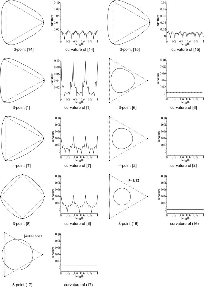

  

  Comparison of existing and proposed SS when three control points are sampled from circle. Left: Limit curves obtained after the 5th iteration, the corresponding curvature is shown in the right column, respectively

• In Fig. 5, four control points are sampled to achieve a limiting circle. It is showed that the limiting circle obtained by SSs (16), (17), and [13] has less tendency to depart from its tangent compared to the limiting curves produced by [2, 3, 5, 7, 8, 14].

  Figure 5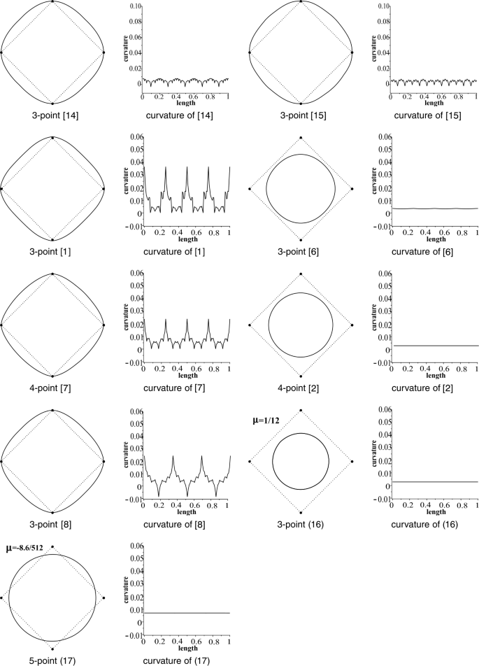

  

  Comparison of existing and proposed SS when four control points are sampled from circle. Left: Limit curves obtained after the 5th iteration, the corresponding curvature is shown in the right column, respectively

• In Fig. 6, five control points are applied to generate a limiting circle. It is observed that the limiting curves obtained by SSs (16), (17), [7], and [13] have less tendency to depart from their tangents compared to the limiting curves produced by [2, 3, 5, 8, 14].

  Figure 6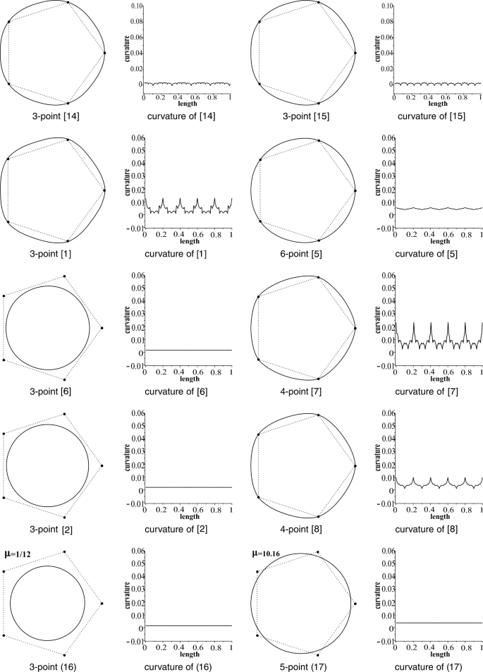

  

  Comparison of existing and proposed SS when five control points are sampled from circle. Left: Limit curves obtained after the 5th iteration, the corresponding curvature is shown in the right column, respectively

• Figures 7 and 8 indicate that curvature and torsion behavior of limiting curves are closely related.

  Figure 7

  

  Results after the 5th iteration of 3-point schemes of [5, 6, 13] and (16) are shown on the left when the initial control points are sampled from Helix. The corresponding curvature and torsion are shown in the center and right columns, respectively

  Figure 8

  

  Results after the 5th iteration of 4-point and 5-point schemes of [8, 14], (17) are shown on the left when the initial control points are sampled from Helix. The corresponding curvature and torsion are shown in the center and right columns, respectively

From the above discussion it is observed that the basic shapes generated by proposed SSs with fewer initial data have less tendency to depart from their tangents as compared to the limiting curves produced by the existing non-stationary subdivision schemes.

5 Conclusions

We offered and analyzed families of $(2s-1)$-point non-stationary subdivision schemes. It is observed that the basic shapes generated by the proposed SSs with fewer initial data in the initial control polygon have less tendency to depart from their tangents as compared to the limiting curves obtained by the existing non-stationary SSs of [2, 3, 5,6,7,8, 13, 14]. It is noticed that SS (17) performed interpolatory role (see Fig. 1(c)). In addition, the proposed SSs are the non-stationary counterparts of the stationary SSs of [5, 11, 12, 22, 24,25,26].

References

Asghar, M., Iqbal, M.J., Mustafa, G.: A family of high continuity subdivision schemes based on probability distribution. Mehran Univ. Res. J. Eng. Technol. 38(2), 389–398 (2019)
Beccari, C., Casciola, G., Romani, L.: A nonstationary uniform tension controlled interpolating 4-point scheme reproducing conics. Comput. Aided Geom. Des. 24(1), 1–9 (2007)
Beccari, C., Casciola, G., Romani, L.: An interpolating 4-point \(C^{2}\) ternary non-stationary subdivision scheme with tension control. Comput. Aided Geom. Des. 24(4), 210–219 (2007)
Conti, C., Romani, L.: A new family of interpolatory non-stationary subdivision schemes for curve design in geometric modeling. AIP Conf. Proc. 1281, 523–526 (2010)
Daniel, S., Shunmugaraj, P.: Three point stationary and non-stationary subdivision schemes. In: 3rd International Conference on Geometric Modeling and Imaging, pp. 3–8 (2008). https://doi.org/10.1109/GMAI.2008.13
Daniel, S., Shunmugaraj, P.: An interpolating 6-point \(C^{2}\) non-stationary subdivision scheme. J. Comput. Appl. Math. 230, 164–172 (2009)
Daniel, S., Shunmugaraj, P.: An approximating \(C^{2}\) non-stationary subdivision scheme. Comput. Aided Geom. Des. 26, 810–821 (2009)
Daniel, S., Shunmugaraj, P.: Some interpolating non-stationary subdivision schemes. In: International Symposium on Computer Science and Society, pp. 400–403 (2011). https://doi.org/10.1109/ISCCS.2011.110
Dyn, N., Levin, D.: Analysis of asymptotically equivalent binary subdivision schemes. J. Math. Anal. Appl. 193, 594–621 (1995)
Dyn, N., Levin, D.: Subdivision scheme in geometric modeling. Acta Numer. 11, 73–144 (2002)
Hassan, M.F., Dodgson, N.A.: Ternary and three-point univariate subdivision schemes. In: Cohen, A., Marrien, J.L., Schumaker, L.L. (eds.) Curve and Surface Fitting: Sant-Malo 2002, pp. 199–208. Nashboro Press, Brentwood (2003)
Hormann, K., Sabin, M.A.: A family of subdivision schemes with cubic precision. Comput. Aided Geom. Des. 25, 41–52 (2008)
Jena, M.K., Shunmugaraj, P., Das, P.C.: A subdivision algorithm for trigonometric spline curves. Comput. Aided Geom. Des. 19, 71–88 (2002)
Jena, M.K., Shunmugaraj, P., Das, P.C.: A non-stationary subdivision scheme for curve interpolation. ANZIAM J. 44, 216–235 (2003)
Kanwal, G., Ghaffar, A., Hafeezullah, M.M., Manan, S.A., Rizwan, M., Rahman, G.: Numerical solution of 2-point boundary value problem by subdivision scheme. Commun. Math. Appl. 10(2), 1–11 (2019)
Li, B., Yu, Z., Yu, B., Su, Z., Liu, X.: Non-stationary subdivision for exponential polynomials reproduction. Acta Math. Appl. Sin. Engl. Ser. 29, 567–578 (2013)
Manan, S.A., Ghaffar, A., Rizwan, M., Rahman, G., Kanwal, G.: A subdivision approach to the approximate solution of 3rd order boundary value problem. Commun. Math. Appl. 9(4), 499–512 (2018)
Mustafa, G., Ejaz, S.T.: A subdivision collocation method for solving two point boundary value problems of order three. J. Appl. Anal. Comput. 7(3), 942–956 (2017)
Mustafa, G., Ghaffar, A., Aslam, M.: A subdivision-regularization framework for preventing over fitting of data by a model. Appl. Appl. Math. Int. J. 8(1), 178–190 (2013)
Mustafa, G., Ghaffar, A., Bari, M.: The \((2n-1)\)-point binary approximating scheme. In: The First International Workshop on Data Management (IWDM 2013), pp. 363–368 (2013). https://doi.org/10.1109/ICDIM.2013.6694036
Mustafa, G., Hameed, R.: Families of univariate and bivariate subdivision schemes originated from quartic B-spline. Adv. Comput. Math. 43(5), 1131–1161 (2017)
Mustafa, G., Khan, F., Ghaffar, A.: The m-point approximating subdivision scheme. Lobachevskii J. Math. 30(2), 138–145 (2009)
Salam, W.U., Siddiqi, S.S., Rehan, K.: Chaikins perturbation subdivision scheme in non-stationary forms. Alex. Eng. J. 55, 2855–2862 (2016)
Siddiqi, S.S., Ahmad, N.: A new three point approximating \(C^{2}\) subdivision scheme. Appl. Math. Lett. 20, 707–711 (2007)
Siddiqi, S.S., Rehan, K.: A stationary binary \(C^{1}\) curve subdivision scheme. Eur. J. Sci. Res. 32(4), 553–561 (2009)
Siddiqi, S.S., Rehan, K.: Modified form of binary and ternary 3-point subdivision scheme. Appl. Math. Comput. 216, 970–982 (2010)
Tan, J., Sun, J., Tong, G.: A non-stationary binary three-point approximating subdivision scheme. Appl. Math. Comput. 276, 37–43 (2016)
Acknowledgements
Not applicable.
Availability of data and materials
Funding
Author information
Authors and Affiliations
Contributions
The authors contributed equally and significantly in writing this paper. All authors read and approved the final manuscript.
Corresponding author
Ethics declarations
Competing interests
The authors declare that they have no competing interests.
Additional information
Publisher’s Note
Springer Nature remains neutral with regard to jurisdictional claims in published maps and institutional affiliations.
Rights and permissions
Open Access This article is distributed under the terms of the Creative Commons Attribution 4.0 International License (http://creativecommons.org/licenses/by/4.0/), which permits unrestricted use, distribution, and reproduction in any medium, provided you give appropriate credit to the original author(s) and the source, provide a link to the Creative Commons license, and indicate if changes were made.
About this article
Cite this article
Ghaffar, A., Ullah, Z., Bari, M. et al. Family of odd point non-stationary subdivision schemes and their applications. Adv Differ Equ 2019, 171 (2019). https://doi.org/10.1186/s13662-019-2105-5
Received:
Accepted:
Published:
DOI: https://doi.org/10.1186/s13662-019-2105-5