Block-pulse functions method for solving three-dimensional fractional Poisson type equations with Neumann boundary conditions

Abstract

In this paper, a numerical scheme based on the three-dimensional block-pulse functions is proposed to solve the three-dimensional fractional Poisson type equations with Neumann boundary conditions. The differential operational matrices of fractional order of the three-dimensional block-pulse functions are derived from one-dimensional block-pulse functions, which are used to reduce the original problem to solve a system of linear algebra equations. In addition, the convergence analysis of the proposed method is deeply investigated. Lastly, several numerical examples are presented and the numerical results obtained show that our method is effective and feasible.

1 Introduction

Fractional calculus is a branch of mathematics which deals with derivatives and integrals of non-integer orders. In recent years, numerous applications of fractional-order ordinary and partial differential equations have appeared in physics and engineering [1–8]. However, since the kernel of these differential equations is fractional, it is extremely difficult to obtain exact solutions. Therefore, extensive research has been performed on the development of numerical methods for fractional differential equations such as the Chebyshev collocation method [9, 10], the Laplace transform method [11, 12], DTM [13, 14], ADM [15, 16], the operational matrices method [17–20], and the wavelets method [21–23].

In this paper, we consider the three-dimensional fractional Poisson type equations of the following form:

$$\begin{aligned} &\frac{\partial^{\alpha} u ( x,y,z )}{\partial x^{\alpha}} + \frac{\partial^{\beta} u ( x,y,z )}{\partial y^{\beta}} + \frac{\partial^{\gamma} u ( x,y,z )}{ \partial z^{\gamma}} = g ( x,y,z ), \\ &\quad ( x,y,z ) \in [ 0,\tau_{1} ) \times [ 0,\tau_{2} ) \times [ 0,\tau_{3} ), \end{aligned}$$

(1)

where $\frac{\partial^{\alpha}}{\partial x^{\alpha}},\frac{\partial^{\beta}}{\partial y^{\beta}},\frac{\partial^{\gamma}}{\partial z^{\gamma}}$ denotes the Caputo derivative, $g ( x,y,z )$ is a known function and $u ( x,y,z )$ is the solution function to be determined. It is subject to the Neumann boundary conditions:

$$ \begin{aligned}& u ( x,y,0 ) = f_{1} ( x,y ),\qquad u ( x,0,z ) = f_{2} ( x,z ),\qquad u ( 0,y,z ) = f_{3} ( y,z ), \\ &\frac{\partial u}{\partial z}\Big| _{ ( x,y,\tau_{3} )} = f_{4} ( x,y ),\qquad \frac{\partial u}{\partial y} \Big| _{ ( x,\tau_{2},z )} = f_{5} ( x,z ),\qquad \frac{\partial u}{\partial x} \Big| _{ ( \tau_{1},y,z )} = f_{6} ( y,z ). \end{aligned} $$

(2)

So far, only few numerical methods were proposed to obtain the approximate solutions of the three-dimensional fractional PDEs and integral equations. In [24], Caratelli and Ricci discussed the Robin problem for the Laplace equation in a three-dimensional starlike domain. Lin Liu and Hong Zhang applied the single layer regularized meshless method for three-dimensional Laplace problems in [25]. In [26–28], the authors utilized the three-dimensional block-pulse functions and Jacobi polynomials to obtain the numerical solutions of three-dimensional integral equations. Based on the above research, a numerical technique based three-dimensional block-pulse functions in our study is proposed to solve three-dimensional fractional Poisson type equations with Neumann boundary conditions.

The paper is organized as follows: In Sect. 2, some basic definitions of fractional calculus are introduced. In Sect. 3, we introduced the three-dimensional block-pulse functions and their properties. The convergence analysis of the three-dimensional block-pulse functions are discussed in Sect. 4. In Sect. 5, we applied the three-dimensional block-pulse functions to solve the three-dimensional fractional Poisson type equations. The numerical solutions are obtained by several examples in Sect. 6. Lastly, a concluding remark is provided in Sect. 7.

2 Basic definitions

In this section we present some necessary definitions and mathematical preliminaries of the fractional calculus theory which are required for establishing our results.

Definition 2.1

A real function $f ( x ),x > 0$, is said to be in the space $C_{\mu},\mu \in \Re$ if there exists a real number $p\ ( > \mu )$ such that $f ( x ) = x^{p}f_{1} ( x )$, where $f_{1} ( x ) \in C [ 0, + \infty ]$ and it is said to be in the space $C_{\mu}^{n}$ if $f^{ ( n )} \in C_{\mu},n \in N^{ +}$.

Definition 2.2

The Riemann–Liouville fractional integration operator of order $\alpha \ge 0$ of a function $f \in C_{\mu},\mu \ge - 1$, is defined as

$$ \bigl( I^{\alpha} f \bigr) ( x ) = \textstyle\begin{cases} \frac{1}{\Gamma ( \alpha )}\int_{0}^{x} ( x - \tau )^{\alpha - 1}\,{d}\tau, &\alpha > 0, \\ f ( x ),& \alpha = 0. \end{cases} $$

(3)

Definition 2.3

The fractional derivative operator of order $\alpha > 0$ in the Caputo sense is defined as

$$ \bigl( D_{*}^{\alpha} f \bigr) ( x ) = \textstyle\begin{cases} \frac{{d}^{n}f ( x )}{{d}x^{n}},& \alpha = n \in N^{ +}, \\ \frac{1}{\Gamma ( n - \alpha )}\int_{0}^{x} ( x - \tau )^{n - \alpha - 1}f^{ ( n )} ( \tau )\,{d}\tau, & 0 < n - 1 \le \alpha < n, \end{cases} $$

(4)

where n is an integer, $x > 0$, and $f \in C_{1}^{n}$.

The useful relation between the Riemann–Liouville operator and Caputo operator is given by the following expression:

$$ \bigl( I^{\alpha} D_{*}^{\alpha} f \bigr) ( x ) = f ( x ) - \sum_{k = 0}^{n - 1} f^{ ( k )} \bigl( 0^{ +} \bigr)\frac{x^{k}}{k!},\quad x > 0, n - 1 < \alpha \le n, $$

(5)

where n is an integer, $x > 0$, and $f \in C_{1}^{n}$.

For more details as regards fractional calculus see [29].

3 Three-dimensional block-pulse functions (3D-BPFs)

3.1 Definition and properties

The $m^{3}$-set of 3D-BPFs consists of $m^{3}$ functions which are defined over district $D = [ 0,\tau_{1} ) \times [ 0,\tau_{2} ) \times [ 0,\tau_{3} )$ as follows [26]:

$$ \phi_{i,j,k} ( x,y,z ) = \textstyle\begin{cases} 1,& ( i - 1 )h_{1} \le x < ih_{1}, ( j - 1 )h_{2} \le y < jh_{2}, ( k - 1 )h_{3} \le z < kh_{3}, \\ 0,& \mbox{otherwise}, \end{cases} $$

(6)

where m is positive integer, and $h_{1} = \frac{\tau_{1}}{m},h_{2} = \frac{\tau_{2}}{m},h_{3} = \frac{\tau_{3}}{m},\tau_{1},\tau_{2},\tau_{3} \in N^{ +}$. Since each 3D-BPF takes only one value in its sub-region, the 3D-BPFs can be expressed by three one-dimensional block-pulse functions (1D-BPFs):

$$ \phi_{i,j,k} ( x,y,z ) = \phi_{i} ( x )\phi_{j} ( y )\phi_{k} ( z ), $$

(7)

where $\phi_{i} ( x ),\phi_{j} ( y )$ and $\phi_{k} ( z )$ are the 1D-BPFs related to the variables $x,y$ and z, respectively. The 3D-BPFs are disjointed with each other:

$$ \phi_{i,j,k} ( x,y,z )\phi_{i',j',k'} ( x,y,z ) = \textstyle\begin{cases} \phi_{i,j,k} ( x,y,z ),& i = i',j = j',k = k' \\ 0, &\mbox{otherwise} \end{cases} $$

(8)

and are orthogonal to each other:

$$ \int_{0}^{\tau_{1}} \int_{0}^{\tau_{2}} \int_{0}^{\tau_{3}} \phi_{i,j,k} ( x,y,z ) \phi_{i',j',k'} ( x,y,z )\,dz\,dy\,dx = \textstyle\begin{cases} h_{1}h_{2}h_{3},& i = i',j = j',k = k' \\ 0,& \mbox{otherwise}. \end{cases} $$

(9)

We consider the first $m^{3}$ terms of 3D-BPFs and write them concisely as $m^{3}$-vector:

$$ \Phi ( x,y,z ) = \bigl[ \phi_{1,1,1} ( x,y,z ), \ldots, \phi_{1,1,m} ( x,y,z ), \ldots,\phi_{1,m,m} ( x,y,z ), \ldots, \phi_{m,m,m} ( x,y,z ) \bigr]^{T}. $$

(10)

3.2 3D-BPFs expansions

A function $f ( x,y,z )$ defined over district $L^{2} ( D )$ may be expanded by the 3D-BPFs:

$$ f ( x,y,z ) \simeq \sum_{i = 1}^{m} \sum _{j = 1}^{m} \sum _{k = 1}^{m} f_{i,j,k}\phi_{i,j,k} ( x,y,z ) = F^{T}\Phi ( x,y,z ) = \Phi ( x,y,z )^{T}F, $$

(11)

where F is an $m^{3} \times 1$ vector given by

$$F = [ f_{1,1,1}, \ldots,f_{1,1,m}, \ldots,f_{1,m,m}, \ldots,f_{m,m,m} ]^{T}, $$

$\Phi ( x,y,z )$ is defined in Eq. (10), and $f_{i,j,k}$, are obtained as

$$ f_{i,j,k} = \frac{1}{h_{1}h_{2}h_{3}} \int_{ ( i - 1 )h_{1}}^{ih_{1}} \int_{ ( j - 1 )h_{2}}^{jh_{2}} \int_{ ( k - 1 )h_{3}}^{kh_{3}} f ( x,y,z )\,{d}z\,{d}y \,{d}x. $$

(12)

3.3 Operational matrix of fractional differentiation

In this part, we may simply introduce the operational matrix of fractional integration of 1D-BPFs, a more detailed introduction can be found in Ref. [30].

Let $\tau_{1} = \tau_{2} = \tau_{3} = \tau$. If $I^{\alpha}$ is fractional integration operator of 1D-BPFs, we can get

$$ I^{\alpha} \Phi ( x ) \simeq P^{\alpha} \Phi ( x ), $$

(13)

where

$$P^{\alpha} = \biggl( \frac{\tau}{m} \biggr)^{\alpha} \frac{1}{\Gamma ( \alpha + 2 )} \left [ \begin{matrix} 1 & \xi_{1} & \xi_{2} & \cdots & \xi_{m - 1} \\ 0 & 1 & \xi_{1} & \cdots & \xi_{m - 2} \\ 0 & 0 & 1 & \cdots & \xi_{m - 3} \\ \vdots & \vdots & \vdots & \ddots & \vdots \\ 0 & 0 & 0 & \cdots & 1 \end{matrix} \right ], $$

where

$$\xi_{k} = ( k + 1 )^{\alpha + 1} - 2k^{\alpha + 1} + ( k - 1 )^{\alpha + 1}, \quad k = 1,2, \ldots,m - 1. $$

$P^{\alpha}$ is called the block-pulse operational matrix of fractional integration.

Let $D^{\alpha}$ be the block-pulse operational matrix for the fractional differentiation. According to the property calculus, $D^{\alpha} P^{\alpha} = I$, we can easily obtain matrix $D^{\alpha}$ by inverting the $P^{\alpha}$ matrix.

4 Convergence analysis of 3D-BPFs

In this section, we show that the given method in the previous sections, is convergent and its order of convergence is $O ( \frac{1}{m} )$. For our purposes we will need the following theorems.

Theorem 1

Assume that

$$f_{m} ( x,y,z ) = \sum_{i = 1}^{m} \sum_{j = 1}^{m} \sum _{k = 1}^{m} f_{i,j,k}\phi_{i,j,k} ( x,y,z ), $$

be the approximate solution of Eq. (1), then

$$\int_{0}^{\tau_{1}} \int_{0}^{\tau_{2}} \int_{0}^{\tau_{3}} \bigl( f ( x,y,z ) - f_{m} ( x,y,z ) \bigr)^{2}\,{d}z\,{d}y\,{d}x, $$

achieves its minimum value. Moreover, we have

$$\int_{0}^{\tau_{1}} \int_{0}^{\tau_{2}} \int_{0}^{\tau_{3}} f^{2} ( x,y,z )\,dz\,dy\,dx = \sum_{i = 1}^{\infty} \sum _{j = 1}^{\infty} \sum_{k = 1}^{\infty} f_{i,j,k}^{2} \bigl\Vert \phi_{i,j,k}^{2} ( x,y,z ) \bigr\Vert ^{2}. $$

Proof

For the proof, see [31]. □

Theorem 2

([32])

Assume that $f_{m} ( x,y,z )$ is the approximate solution of Eq. (1). If $f ( x,y,z )$ is the exact solution of Eq. (1), then we have

$$\lim_{m \to \infty} f_{m} ( x,y,z ) = f ( x,y,z ) $$

and

$$\bigl\Vert e ( x,y,z ) \bigr\Vert = \bigl\Vert f ( x,y,z ) - f_{m} ( x,y,z ) \bigr\Vert = O \biggl( \frac{1}{m} \biggr). $$

The proof is in the Appendix.

5 Numerical implementation

In this section, we apply the three-dimensional block-pulse functions for solving three-dimensional fractional Poisson type equations with Neumann boundary conditions. We firstly approximate the function $u ( x,y,z )$ by 3D-BPFs:

$$ u ( x,y,z ) \simeq \Phi ( x,y,z )^{T}U, $$

(14)

where

$$U = [ u_{1,1,1}, \ldots,u_{1,1,m}, \ldots,u_{1,m,m}, \ldots,u_{m,m,m} ]_{m^{3} \times 1}^{T}. $$

According to Eq. (7) and Eq. (10), we have

$$ \Phi ( x,y,z ) = \Phi ( x ) \otimes \bigl( \Phi ( y ) \otimes \Phi ( z ) \bigr), $$

(15)

where ⊗ is the Kronecker product, and

$$\begin{aligned}& \Phi ( x ) = \bigl[ \phi_{1} ( x ),\phi_{2} ( x ), \ldots,\phi_{m} ( x ) \bigr]^{T},\qquad \Phi ( y ) = \bigl[ \phi_{1} ( y ),\phi_{2} ( y ), \ldots,\phi_{m} ( y ) \bigr]^{T}, \\ &\Phi ( z ) = \bigl[ \phi_{1} ( z ),\phi_{2} ( z ), \ldots, \phi_{m} ( z ) \bigr]^{T}. \end{aligned} $$

Here $\Phi ( x ),\Phi ( y )$ and $\Phi ( z )$ are m-vectors. Then we have [18]

$$\begin{aligned} \frac{\partial^{\alpha} u ( x,y,z )}{\partial x^{\alpha}}& \simeq \frac{\partial^{\alpha} \Phi ( x,y,z )^{T}}{\partial x^{\alpha}} U \\ &= \biggl\{ \biggl( \frac{\partial^{\alpha} \Phi ( x )}{\partial x^{\alpha}} \biggr) \otimes \bigl( \Phi ( y ) \otimes \Phi ( z ) \bigr) \biggr\} ^{T}U \\ &= \bigl\{ \bigl( D^{\alpha} \Phi ( x ) \bigr) \otimes \bigl( \Phi ( y ) \otimes \Phi ( z ) \bigr) \bigr\} ^{T}U \\ &= \Phi ( x,y,z )^{T} \bigl( D^{\alpha} \otimes I_{1} \bigr)^{T}U, \end{aligned}$$

(16)

$$\begin{aligned} \frac{\partial^{\beta} u ( x,y,z )}{\partial y^{\beta}}& \simeq \frac{\partial^{\beta} \Phi ( x,y,z )^{T}}{\partial y^{\beta}} U \\ & = \biggl\{ \Phi ( x ) \otimes \biggl( \biggl( \frac{\partial^{\beta} \Phi ( y )}{\partial y^{\beta}} \biggr) \otimes \Phi ( z ) \biggr) \biggr\} ^{T}U \\ &= \bigl\{ \Phi ( x ) \otimes \bigl( \bigl( D^{\beta} \Phi ( y ) \bigr) \otimes \Phi ( z ) \bigr) \bigr\} ^{T}U \\ & = \Phi ( x,y,z )^{T} \bigl\{ I_{2} \otimes \bigl( D^{\beta} \otimes I_{2} \bigr) \bigr\} ^{T}U, \end{aligned}$$

(17)

and

$$\begin{aligned} \frac{\partial^{\gamma} u ( x,y,z )}{\partial z^{\gamma}}& \simeq \frac{\partial^{\gamma} \Phi ( x,y,z )^{T}}{\partial z^{\gamma}} U \\ &= \biggl\{ \Phi ( x ) \otimes \biggl( \Phi ( y ) \otimes \frac{\partial^{\gamma} \Phi ( z )}{\partial z^{\gamma}} \biggr) \biggr\} ^{T}U \\ & = \bigl\{ \bigl( \Phi ( x ) \otimes \Phi ( y ) \bigr) \otimes \bigl( D^{\gamma} \Phi ( z ) \bigr) \bigr\} ^{T}U \\ & = \Phi ( x,y,z )^{T} \bigl( I_{1} \otimes D^{\gamma} \bigr)^{T}U. \end{aligned}$$

(18)

where $I_{1}$ and $I_{2}$ are $m^{2} \times m^{2}$ and $m \times m$ identity matrices, respectively. Substituting Eqs. (16)–(18) into Eq. (1), we have

$$\begin{aligned} &\Phi ( x,y,z )^{T} \bigl( D^{\alpha} \otimes I_{1} \bigr)^{T}U + \Phi ( x,y,z )^{T} \bigl\{ I_{2} \otimes \bigl( D^{\beta} \otimes I_{2} \bigr) \bigr\} ^{T}U + \Phi ( x,y,z )^{T} \bigl( I_{1} \otimes D^{\gamma} \bigr)^{T}U \\ &\quad = g ( x,y,z ), \end{aligned}$$

(19)

and similar to Eq. (19), we have by Eq. (2)

$$ \begin{aligned} &\Phi ( x,y,0 )^{T}U = f_{1} ( x,y ),\qquad \Phi ( x,0,z )^{T}U = f_{2} ( x,z ),\qquad \Phi ( 0,y,z )^{T}U = f_{3} ( y,z ), \\ &\Phi ( x,y,\tau_{3} )^{T} \bigl( I_{1} \otimes D^{1} \bigr)^{T}U = f_{4} ( x,y ),\qquad \Phi ( x, \tau_{2},z )^{T} \bigl\{ I_{2} \otimes \bigl( D^{1} \otimes I_{2} \bigr) \bigr\} ^{T}U = f_{5} ( x,z ), \\ &\Phi ( \tau_{1},y,z )^{T} \bigl( D^{1} \otimes I_{1} \bigr)^{T}U = f_{6} ( y,z ). \end{aligned} $$

(20)

Here $D^{1}$ denotes the operational matrix of first order. Equation (19) together with Eq. (20) constitutes a system of algebraic equations. Take the collocation method to disperse the unknown variables $x,y,z$ in the following form:

$$ x_{i} = \frac{\tau_{1} ( 2i - 1 )}{2m},\qquad y_{j} = \frac{\tau_{2} ( 2j - 1 )}{2m},\qquad z_{k} = \frac{\tau_{3} ( 2k - 1 )}{2m},\quad i,j,k = 1, \ldots,m. $$

(21)

Then we have

$$ \textstyle\begin{cases} \Phi ( x_{i},y_{j},z_{k} )^{T} ( D^{\alpha} \otimes I_{1} )^{T}U + \Phi ( x_{i},y_{j},z_{k} )^{T} \{ I_{2} \otimes ( D^{\beta} \otimes I_{2} ) \}^{T}U \\ \qquad{}+ \Phi ( x_{i},y_{j},z_{k} )^{T} ( I_{1} \otimes D^{\gamma} )^{T}U \\ \quad{}= g ( x_{i},y_{j},z_{k} ), \\ \Phi ( x_{i},y_{j},0 )^{T}U = f_{1} ( x_{i},y_{j} ),\qquad \Phi ( x_{i},0,z_{k} )^{T}U = f_{2} ( x_{i},z_{k} ),\\ \Phi ( 0,y_{j},z_{k} )^{T}U = f_{3} ( y_{j},z_{k} ), \\ \Phi ( x_{i},y_{j},\tau_{3} )^{T} ( I_{1} \otimes D^{1} )^{T}U = f_{4} ( x_{i},y_{j} ),\\ \Phi ( x_{i},\tau_{2},z_{k} )^{T} \{ I_{2} \otimes ( D^{1} \otimes I_{2} ) \}^{T}U = f_{5} ( x_{i},z_{k} ), \\ \Phi ( \tau_{1},y_{j},z_{k} )^{T} ( D^{1} \otimes I_{1} )^{T}U = f_{6} ( y_{j},z_{k} ). \end{cases} $$

(22)

By solving the linear system of Eq. (22), the coefficient matrix U can be found. Then substituting it into (14), the unknown solution can be obtained.

6 Numerical examples

To demonstrate the efficiency and the practicability of the proposed method via three-dimensional block-pulse functions, we consider the following several numerical examples.

Example 6.1

Consider the following three-dimensional fractional-order PDE:

$$\begin{aligned} &\frac{\partial^{1.5}u ( x,y,z )}{\partial x^{1.5}} + \frac{\partial^{1.5}u ( x,y,z )}{\partial y^{1.5}} + \frac{\partial^{1.5}u ( x,y,z )}{\partial z^{1.5}} = g ( x,y,z ), \\ &\quad ( x,y,z ) \in [ 0,2 ) \times [ 0,2 ) \times [ 0,2 ), \end{aligned}$$

(23)

where $g ( x,y,z ) = 4 ( x^{0.5}y^{2}z^{2} + x^{2}y^{0.5}z^{2} + x^{2}y^{2}z^{0.5} ) / \sqrt{\pi}$, with the Neumann boundary conditions: $u ( 0,y,z ) = u ( x,0,z ) = u ( x,y,0 ) = 0,\frac{\partial u}{\partial x} | _{x = 2} = 4yz,\frac{\partial u}{\partial y} | _{y = 2} = 4xz,\frac{\partial u}{\partial z} | _{z = 2} = 4xy$. The analytical solution for the system is $u ( x,y,z ) = x^{2}y^{2}z^{2}$. The absolute errors for $m = 16,32$ and 64 in some nodes $( x,y,z )$ are shown in Table 1. Tables 1 and 2 show that our proposed scheme can achieve a good convergence result as m increases.

Table 1 The absolute error in some nodes of $x,y$ and z when $m = 16,32$ and 64 for Example 6.1

Table 2 The numerical and analytical solutions with $m = 8,16,32$ at some values of $x,y,z$ for Example 6.2

Example 6.2

Consider the following fractional three-dimensional Poisson equation:

$$\begin{aligned} &\frac{\partial^{1.75}u ( x,y,z )}{\partial x^{1.75}} + \frac{\partial^{1.5}u ( x,y,z )}{\partial y^{1.5}} + \frac{\partial^{1.25}u ( x,y,z )}{\partial z^{1.25}} = g ( x,y,z ), \\ &\quad ( x,y,z ) \in [ 0,1 ) \times [ 0,1 ) \times [ 0,1 ), \end{aligned}$$

(24)

where $g ( x,y,z ) = - \frac{2}{\Gamma ( 1.25 )}x^{0.25}yz ( 2 - y ) ( 2 - z ) - \frac{2}{\Gamma ( 1.5 )}xy^{0.5}z ( 2 - x ) ( 2 - z ) - \frac{2}{\Gamma ( 1.75 )}xyz^{0.75} ( 2 - x ) ( 2 - y )$, with the Neumann boundary conditions: $u ( 0,y,z ) = u ( x,0,z ) = u ( x,y,0 ) = \frac{\partial u}{\partial x} | _{x = 1} = \frac{\partial u}{\partial y} | _{y = 1} = \frac{\partial u}{\partial z} | _{z = 1} = 0$. The analytical solution of this problem is $u ( x,y,z ) = xyz ( 2 - x ) ( 2 - y ) ( 2 - z )$. When $m = 8,16,32$, the numerical and analytical solutions at some values of $x,y,z$ are given in Table 2.

Example 6.3

We consider the following three-dimensional second-order Poisson equation:

$$\begin{aligned} &\frac{\partial^{2}u ( x,y,z )}{\partial x^{2}} + \frac{\partial^{2}u ( x,y,z )}{\partial y^{2}} + \frac{\partial^{2}u ( x,y,z )}{\partial z^{2}} = g ( x,y,z ), \\ &\quad ( x,y,z ) \in [ 0,2\pi ) \times [ 0,2\pi ) \times [ 0,2\pi ), \end{aligned}$$

(25)

where $g ( x,y,z ) = - 3\sin ( x + \frac{\pi}{2} )\sin ( y + \frac{\pi}{2} )\sin ( z + \frac{\pi}{2} )$, subject to the Neumann boundary conditions: $u ( 0,y,z ) = \sin ( y + \frac{\pi}{2} )\sin ( z + \frac{\pi}{2} ),u ( x,0,z ) = \sin ( x + \frac{\pi}{2} )\sin ( z + \frac{\pi}{2} )$, $u ( x,y,0 ) = \sin ( x + \frac{\pi}{2} )\sin ( z + \frac{\pi}{ 2} ),\frac{\partial u}{\partial x}| _{x = 2\pi} = \frac{\partial u}{\partial y}| _{y = 2\pi} = \frac{\partial u}{\partial z}| _{z = 2\pi} = 0$. The analytical solution for the system is $u ( x,y,z ) = \sin ( x + \frac{\pi}{2} )\sin ( y + \frac{\pi}{2} )\sin ( z + \frac{\pi}{2} )$. When $z = \pi$, the graphs of the approximate solutions for $m = 16,32$ and 64 are shown in Figs. 1–3. The graph of the analytical solution is shown in Fig. 4. The graph of the absolute error with $m = 64$ is shown in Fig. 5. From Figs. 1–5, it can be concluded that the approximate solutions approach the analytical solutions well as m grows.

Figure 1

The approximate solution $u ( x,y,\pi )$ with $m = 16$ for Example 6.3

Figure 2

The approximate solution $u ( x,y,\pi )$ with $m = 32$ for Example 6.3

Figure 3

The approximate solution $u ( x,y,\pi )$ with $m = 64$ for Example 6.3

Figure 4

Analytical solution $u ( x,y,\pi )$ for Example 6.3

Figure 5

Absolute error $e ( x,y,\pi )$ for Example 6.3

Example 6.4

Consider the following three-dimensional fractional-order Poisson equation:

$$\begin{aligned} &\frac{\partial^{\alpha} u ( x,y,z )}{\partial x^{\alpha}} + \frac{\partial^{\beta} u ( x,y,z )}{\partial y^{\beta}} + \frac{\partial^{\gamma} u ( x,y,z )}{\partial z^{\gamma}} = g ( x,y,z ), \\ &\quad ( x,y,z ) \in [ 0,1 ) \times [ 0,1 ) \times [ 0,1 ), \end{aligned}$$

(26)

where $g ( x,y,z ) = 3 ( e^{x} - 1 ) ( e^{y} - 1 ) ( e^{z} - 1 )$, subject to the Neumann boundary conditions: $u ( 0,y,z ) = u ( x,0,z ) = u ( x,y,0 ) = 0,\frac{\partial u}{\partial x} | _{x = 1} = ( e - 1 ) ( e^{y} - 1 ) ( e^{z} - 1 ),\frac{\partial u}{\partial y} | _{y = 1} = ( e - 1 ) ( e^{x} - 1 ) ( e^{z} - 1 ), \frac{\partial u}{\partial z} | _{z = 1} = ( e - 1 ) ( e^{x} - 1 ) ( e^{y} - 1 )$. The analytical solution of this system for $\alpha = \beta = \gamma = 2$ is $u ( x,y,z ) = ( e^{x} - 1 ) ( e^{y} - 1 ) ( e^{z} - 1 )$.

• (i) When $z = 0.5$, the numerical and analytical solutions for $m = 64$ at $y = 0.3,0.6,0.9$ are shown in Fig. 6.

  Figure 6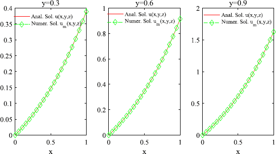

  

  The numerical and analytical solution with $m = 64$ at $y = 0.3,0.6,0.9$ for Example 6.4

• (ii) When $z = 0.5$, the absolute errors for $m = 64$ at $y = 0.3,0.6,0.9$ are shown in Fig. 7.

  Figure 7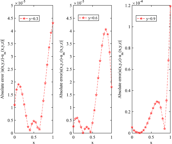

  

  The absolute error with $m = 64$ at $y = 0.3,0.6,0.9$ for Example 6.4

Example 6.5

Consider Eq. (26), when $m = 32$, the graphs of the numerical solutions with $\alpha = \beta = \gamma = 1.95,\alpha = \beta = \gamma = 1.90,\alpha = \beta = \gamma = 1.85$ at $x = 0.3,y = 0.6$ are shown in Fig. 8, which shows that the approximate solutions are well in agreement with the analytical solution as the fractional orders $\alpha,\beta,\gamma$ gradually approximate 2. The robustness of the proposed method is tested in this example.

Figure 8

The numerical solutions with different fractional order $\alpha,\beta,\gamma$ when $m = 32$ for Example 6.5

7 Conclusions

In this paper, we have studied a numerical scheme to solve three-dimensional fractional Poisson type problems with Neumann boundary conditions. Our approach was based on the 3D-BPFs and their operational matrix of fractional differentiation together with a set of suitable collocation nodes. This method reduces the amount of computation of this problem using the collocation nodes assigned to approximate solution. The typical convergence rate of the method is $O ( \frac{1}{m} )$ as shown in the numerical results. Moreover, they show that our proposed method is effective and robust.

Appendix

Proof

We assume that $f ( x,y,z )$ is a differentiable function on D such that

$$\bigl\Vert f ( x,y,z ) \bigr\Vert \le M. $$

We define the representation error between $f ( x,y,z )$ and its 3D-BPFs expansion, $f_{m} ( x,y,z )$ over every sub-region $D_{i,j,k}$ as follows:

$$e_{i,j,k} ( x,y,z ) = f ( x,y,z ) - f_{i,j,k}\phi_{i,j,k} ( x,y,z ) = f ( x,y,z ) - f_{i,j,k},\quad ( x,y,z ) \in D_{i,j,k}, $$

where

$$D_{i,j,k} = \bigl\{ ( i - 1 )h_{1} \le x < ih_{1}, ( j - 1 )h_{2} \le y < jh_{2}, ( k - 1 )h_{3} \le z < kh_{3} \bigr\} . $$

It can be shown that

$$\begin{aligned} \bigl\Vert e_{i,j,k} ( x,y,z ) \bigr\Vert ^{2}& = \int_{ ( i - 1 )h_{1}}^{ih_{1}} \int_{ ( j - 1 )h_{2}}^{jh_{2}} \int_{ ( k - 1 )h_{3}}^{kh_{3}} e_{i,j,k}^{2} ( x,y,z )\,{d}z\,{d}y\,{d}x \\ &= \int_{ ( i - 1 )h_{1}}^{ih_{1}} \int_{ ( j - 1 )h_{2}}^{jh_{2}} \int_{ ( k - 1 )h_{3}}^{kh_{3}} \bigl( f ( x,y,z ) - f_{i,j,k} \bigr)^{2}\,{d}z\,{d}y\,{d}x \\ &= \frac{\tau_{1}\tau_{2}\tau_{3}}{m^{3}} \bigl( f ( \eta_{1},\eta_{2}, \eta_{3} ) - f_{i,j,k} \bigr)^{2};\quad ( \eta_{1},\eta_{2},\eta_{3} ) \in D_{i,j,k}, \end{aligned}$$

(27)

where we used mean value theorem for 3D integrals. Using Eq. (12) and the mean value theorem we have

$$\begin{aligned} f_{i,j,k} &= m^{3} \int_{ ( i - 1 )h_{1}}^{ih_{1}} \int_{ ( j - 1 )h_{2}}^{jh_{2}} \int_{ ( k - 1 )h_{3}}^{kh_{3}} f ( x,y,z )\,{d}z\,{d}y \,{d}x \\ & = m^{3} \cdot \frac{\tau_{1}\tau_{2}\tau_{3}}{m^{3}}f ( \xi_{1}, \xi_{2},\xi_{3} );\quad ( \xi_{1},\xi_{2}, \xi_{3} ) \in D_{i,j,k}. \end{aligned}$$

(28)

Substituting above relation into Eq. (27) and using Theorem 1 we obtain

$$\begin{aligned} &\bigl\Vert e_{i,j,k} ( x,y,z ) \bigr\Vert ^{2} \\ &\quad= \frac{\tau_{1}\tau_{2}\tau_{3}}{m^{3}} \bigl( f ( \eta_{1},\eta_{2}, \eta_{3} ) - f ( \xi_{1},\xi_{2}, \xi_{3} ) \bigr)^{2} \le \frac{\tau_{1}\tau_{2}\tau_{3}M^{2}}{m^{3}} \bigl\vert ( \eta_{1},\eta_{2},\eta_{3} ) - ( \xi_{1},\xi_{2},\xi_{3} ) \bigr\vert ^{2} \\ &\quad \le \frac{\tau_{1}\tau_{2}\tau_{3} ( \tau_{1} + \tau_{2} + \tau_{3} )}{m^{5}}M^{2}. \end{aligned}$$

This leads to

$$\begin{aligned} &\bigl\Vert e ( x,y,x ) \bigr\Vert ^{2} \\ &\quad\le \int_{0}^{\tau_{1}} \int_{0}^{\tau_{2}} \int_{0}^{\tau_{3}} e^{2} ( x,y,z ) \,{d}z \,{d}y\,{d}x \\ &\quad= \int_{0}^{\tau_{1}} \int_{0}^{\tau_{2}} \int_{0}^{\tau_{3}} \Biggl( \sum _{i = 1}^{m} \sum_{j = 1}^{m} \sum_{k = 1}^{m} e_{i,j,k} ( x,y,z ) \Biggr)^{2}\,{d}z\,{d}y\,{d}x \\ &\quad = \int_{0}^{\tau_{1}} \int_{0}^{\tau_{2}} \int_{0}^{\tau_{3}} \sum_{i = 1}^{m} \sum_{j = 1}^{m} \sum _{k = 1}^{m} e_{i,j,k}^{2} ( x,y,z ) \,{d}z\,{d}y\,{d}x \\ &\qquad{}+ 2\sum_{i < i'} \sum _{j < j'} \sum_{k < k'} \int_{0}^{\tau_{1}} \int_{0}^{\tau_{2}} \int_{0}^{\tau_{3}} e_{i,j,k} ( x,y,z )e_{i',j',k'} ( x,y,x )\,{d}z\,{d}y\,{d}x. \end{aligned}$$

Since for $i < i';j < j';k < k'$,

$$D_{i,j,k} \cap D_{i',j',k'} = \{\cdot \}, $$

we have

$$\begin{aligned} \bigl\Vert e ( x,y,z ) \bigr\Vert ^{2} = {}&\sum _{i = 1}^{m} \sum_{j = 1}^{m} \sum_{k = 1}^{m} \int_{0}^{\tau_{1}} \int_{0}^{\tau_{2}} \int_{0}^{\tau_{3}} e_{i,j,k}^{2} ( x,y,z )\,{d}z\,{d}y\,{d}x \\ = {}&\sum_{i = 1}^{m} \sum_{j = 1}^{m} \sum _{k = 1}^{m} \Vert e_{i,j,k} \Vert ^{2} \le m^{3}\frac{\tau_{1}\tau_{2}\tau_{3} ( \tau_{1} + \tau_{2} + \tau_{3} )}{m^{5}}M^{2}, \end{aligned}$$

(29)

hence $\Vert e ( x,y,z ) \Vert = O ( \frac{1}{m} )$. Now suppose that $f ( x,y,z )$ is approximated by

$$f_{m} ( x,y,z ) = \sum_{i = 1}^{m} \sum_{j = 1}^{m} \sum _{k = 1}^{m} f_{i,j,k} ( x,y,z ) \phi_{i,j,k} ( x,y,z ), $$

whereas we find $\bar{f}_{i,j,k}$, the approximation of $f_{i,j,k}$, and

$$\bar{f}_{m} ( x,y,z ) = \sum_{i = 1}^{m} \sum_{j = 1}^{m} \sum _{k = 1}^{m} \bar{f}_{i,j,k}\phi_{i,j,k} ( x,y,z ), $$

then for $( x,y,z ) \in D_{i,j,k}$ we have

$$\begin{aligned} &\bigl\Vert \bar{f}_{i,j,k}\phi_{i,j,k} ( x,y,z ) - f ( x,y,z ) \bigr\Vert \\ &\quad= \bigl\Vert \bar{f}_{i,j,k}\phi_{i,j,k} ( x,y,z ) - f ( x,y,z ) + f_{i,j,k}\phi_{i,j,k} ( x,y,z ) - f_{i,j,k} \phi_{i,j,k} ( x,y,z ) \bigr\Vert \\ &\quad\le \bigl\Vert f_{i,j,k}\phi_{i,j,k} ( x,y,z ) - f ( x,y,z ) \bigr\Vert + \bigl\Vert \bar{f}_{i,j,k}\phi_{i,j,k} ( x,y,z ) - f_{i,j,k}\phi_{i,j,k} ( x,y,z ) \bigr\Vert . \end{aligned}$$

(30)

We have

$$\begin{aligned} &\bigl\Vert \bar{f}_{i,j,k}\phi_{i,j,k} ( x,y,z ) - f_{i,j,k}\phi_{i,j,k} ( x,y,z ) \bigr\Vert \\ &\quad = \biggl( \int_{ ( i - 1 )h_{1}}^{ih_{1}} \int_{ ( j - 1 )h_{2}}^{jh_{2}} \int_{ ( k - 1 )h_{3}}^{kh_{3}} \bigl( \bar{f}_{i,j,k} \phi_{i,j,k} ( x,y,z ) - f_{i,j,k}\phi_{i,j,k} ( x,y,z ) \bigr) \biggr)^{\frac{1}{2}} \\ &\quad\le \vert \bar{f}_{i,j,k} - f_{i,j,k} \vert \biggl( \int_{ ( i - 1 )h_{1}}^{ih_{1}} \int_{ ( j - 1 )h_{2}}^{jh_{2}} \int_{ ( k - 1 )h_{3}}^{kh_{3}} \,{d}z\,{d}y\,{d}x \biggr)^{\frac{1}{2}} \\ &\quad= \frac{ ( \tau_{1}\tau_{2}\tau_{2} )^{\frac{1}{2}} \Vert \bar{f}_{i,j,k} - f_{i,j,k} \Vert }{m^{\frac{3}{2}}} \le \frac{ ( \tau_{1}\tau_{2}\tau_{2} )^{\frac{1}{2}} \Vert \bar{f}_{i,j,k} - f_{i,j,k} \Vert _{\infty}}{ m^{\frac{3}{2}}}. \end{aligned}$$

(31)

Having Eqs. (29)–(31), we find the following error bound:

$$\begin{aligned} &\bigl\Vert \bar{f}_{i,j,k}\phi_{i,j,k} ( x,y,z ) - f ( x,y,z ) \bigr\Vert \\ &\quad\le \frac{ [ \tau_{1}\tau_{2}\tau_{3} ( \tau_{1} + \tau_{2} + \tau_{3} ) ]^{\frac{1}{2}}M}{m} + \frac{ ( \tau_{1}\tau_{2}\tau_{2} )^{\frac{1}{2}} \Vert \bar{f}_{i,j,k} - f_{i,j,k} \Vert _{\infty}}{m^{\frac{3}{2}}}, \end{aligned}$$

(32)

and finally from (32), we get

$$\lim_{m \to \infty} f_{m} ( x,y,z ) = f ( x,y,z ). $$

 □

References

Engheta, N.: On fractional calculus and fractional multipoles in electromagnetism. IEEE Trans. Antennas Propag. 44(4), 554–566 (1996)
Bagley, R.L., Torvik, P.J.: Fractional calculus in the transient analysis of viscoelastically damped structures. AIAA J. 23(6), 918–925 (1985)
Kulish, V.V., Lage, J.L.: Application of fractional calculus to fluid mechanics. J. Fluids Eng. 124(3), 803–806 (2002)
Lederman, C., Roquejoffre, J.M., Wolanski, N.: Mathematical justification of a nonlinear integro-differential equation for the propagation of spherical flames. Ann. Mat. Pura Appl. 183(2), 173–239 (2004)
Mainardi, F.: Fractional calculus: some basic problems in continuum and statistical mechanics. In: Fractals Fract. Calc. Contin. Mech., pp. 291–348 (1997)
Meral, F.C., Royston, T.J., Magin, R.: Fractional calculus in viscoelasticity: an experimental study. Commun. Nonlinear Sci. Numer. Simul. 15(4), 939–945 (2010)
Li, Y.Y., Zhao, Y., Xie, G.N., et al.: Local fractional Poisson and Laplace equations with applications to electrostatics in fractal domain. Adv. Math. Phys. 2014, 590574 (2014)
Marin, M., Baleanu, D.: On vibrations in thermoelasticity without energy dissipation for micropolar bodies. Bound. Value Probl. 2016(1), 1 (2016)
Khader, M.M., Sweilam, N.H., Mahdy, A.M.S.: Numerical study for the fractional differential equations generated by optimization problem using Chebyshev collocation method and FDM. Appl. Math. Inf. Sci. 7(5), 2011–2018 (2013)
Baseri, A., Abbasbandy, S., Babolian, E.: A collocation method for fractional diffusion equation in a long time with Chebyshev functions. Appl. Math. Comput. 322, 55–65 (2018)
Kazem, S.: Exact solution of some linear fractional differential equations by Laplace transform. Int. J. Nonlinear Sci. 16(1), 3–11 (2013)
Gupta, S., Kumar, D., Singh, J.: Numerical study for systems of fractional differential equations via Laplace transform. J. Egypt. Math. Soc. 23(2), 256–262 (2015)
Ertürk, V.S., Momani, S.: Solving systems of fractional differential equations using differential transform method. J. Comput. Appl. Math. 215(1), 142–151 (2008)
Yang, X.J., Machado, J.A.T., Srivastava, H.M.: A new numerical technique for solving the local fractional diffusion equation: two-dimensional extended differential transform approach. Appl. Math. Comput. 274, 143–151 (2016)
Momani, S., Al-Khaled, K.: Numerical solutions for systems of fractional differential equations by the decomposition method. Appl. Math. Comput. 162(3), 1351–1365 (2005)
El-Wakil, S.A., Abdou, M.A., Elhanbaly, A.: Adomian decomposition method for solving the diffusion–convection–reaction equations. Appl. Math. Comput. 177(2), 729–736 (2006)
Saadatmandi, A., Dehghan, M.: A new operational matrix for solving fractional-order differential equations. Comput. Math. Appl. 59(3), 1326–1336 (2010)
Xie, J., Huang, Q., Xia, Y.: Numerical solution of the one-dimensional fractional convection diffusion equations based on Chebyshev operational matrix. SpringerPlus 5(1), 1149 (2016)
Xie, J., Huang, Q., Zhao, F., et al.: Block pulse functions for solving fractional Poisson type equations with Dirichlet and Neumann boundary conditions. Bound. Value Probl. 2017, 32 (2017)
Zhao, F., Huang, Q., Xie, J., et al.: Chebyshev polynomials approach for numerically solving system of two-dimensional fractional PDEs and convergence analysis. Appl. Math. Comput. 313, 321–330 (2017)
Saeedi, H., Moghadam, M.M.: Numerical solution of nonlinear Volterra integro-differential equations of arbitrary order by CAS wavelets. Commun. Nonlinear Sci. Numer. Simul. 16(3), 1216–1226 (2011)
Yi, M., Wang, L., Huang, J.: Legendre wavelets method for the numerical solution of fractional integro-differential equations with weakly singular kernel. Appl. Math. Model. 40(4), 3422–3437 (2016)
Aziz, I., Haar, A.M.: Wavelet collocation method for three-dimensional elliptic partial differential equations. Comput. Math. Appl. 73(9), 2023–2034 (2017)
Caratelli, D., Ricci, P.E., Gielis, J.: The Robin problem for the Laplace equation in a three-dimensional starlike domain. Appl. Math. Comput. 218(3), 713–719 (2011)
Liu, L., Zhang, H.: Single layer regularized meshless method for three dimensional Laplace problem. Eng. Anal. Bound. Elem. 71, 164–168 (2016)
Mirzaee, F., Hadadiyan, E., Bimesl, S.: Numerical solution for three-dimensional nonlinear mixed Volterra–Fredholm integral equations via three-dimensional block-pulse functions. Appl. Math. Comput. 237, 168–175 (2014)
Mirzaee, F., Hadadiyan, E.: Applying the modified block-pulse functions to solve the three-dimensional Volterra–Fredholm integral equations. Appl. Math. Comput. 265, 759–767 (2015)
Sadri, K., Amini, A., Cheng, C.: Low cost numerical solution for three-dimensional linear and nonlinear integral equations via three-dimensional Jacobi polynomials. J. Comput. Appl. Math. 319, 493–513 (2017)
Podlubny, I.: Fractional Differential Equations: An Introduction to Fractional Derivatives, Fractional Differential Equations, to Methods of Their Solution and Some of Their Applications. Academic Press, San Diego (1998)
Li, Y., Sun, N.: Numerical solution of fractional differential equations using the generalized block pulse operational matrix. Comput. Math. Appl. 62(3), 1046–1054 (2011)
Jiang, Z., Schoufelberger, W., Thoma, M.: Block Pulse Functions and Their Applications in Control Systems. Springer, New York (1992)
Acknowledgements
This work was supported by the Collaborative Innovation Center of Taiyuan Heavy Machinery Equipment.
Availability of data and materials
Not applicable.
Funding
Author information
Authors and Affiliations
Contributions
XJQ carried out the study and drafted the manuscript. YZB approved the initial and revised version. WRR carried out the numerical experiments and language polishing. DXF and ZJ provided the support of the project. All authors read and approved the final manuscript.
Corresponding author
Ethics declarations
Ethics approval and consent to participate
Competing interests
The authors declare that they have no competing interests.
Consent for publication
Additional information
Publisher’s Note
Springer Nature remains neutral with regard to jurisdictional claims in published maps and institutional affiliations.