Eigenvalues of higher order Sturm-Liouville boundary value problems with derivatives in nonlinear terms

Abstract

We shall consider the Sturm-Liouville boundary value problem $y^{(m)}(t)+\lambda F (t,y(t),y'(t),\ldots, y^{(q)}(t) )=0$, $t\in (0,1)$, $y^{(k)}(0)=0$, $0\leq k\leq m-3$, $\zeta y^{(m-2)}(0)-\theta y^{(m-1)}(0)=0$, $\rho y^{(m-2)}(1)+\delta y^{(m-1)}(1)=0$ where $m\geq3$, $1\leq q\leq m-2$, and $\lambda>0$. It is noted that the boundary value problem considered has a derivative-dependent nonlinear term, which makes the investigation much more challenging. In this paper we shall develop a new technique to characterize the eigenvalues λ so that the boundary value problem has a positive solution. Explicit eigenvalue intervals are also established. Some examples are included to dwell upon the usefulness of the results obtained.

1 Introduction

In this paper we shall consider the higher order Sturm-Liouville boundary value problem

$$ \left \{ \begin{array}{@{}l} y^{(m)}(t)+\lambda F (t,y(t),y'(t),\ldots,y^{(q)}(t) )=0,\quad t\in (0,1),\\ y^{(k)}(0)=0, \quad 0\leq k\leq m-3, \\ \zeta y^{(m-2)}(0)-\theta y^{(m-1)}(0)=0,\qquad \rho y^{(m-2)}(1)+\delta y^{(m-1)}(1)=0, \end{array} \right . $$

(1.1)

where $m\geq3$, $1\leq q\leq m-2$, $\lambda>0$, and F is continuous at least in the domain of interest. The constants ζ, θ, ρ, and δ are such that

$$ \theta\geq0, \qquad\delta\geq0, \qquad\theta+\zeta>0,\qquad \delta+\rho>0,\qquad \kappa\equiv \zeta\rho+ \zeta\delta+\theta\rho>0. $$

(1.2)

These assumptions allow ζ and ρ to be negative.

A vast amount of research has been done on the existence of positive solutions of Sturm-Liouville boundary value problems. The general interest in (1.1) may stem from the fact that the boundary value problem models a wide spectrum of nonlinear phenomena, such as gas diffusion through porous media, nonlinear diffusion generated by nonlinear sources, thermal self ignition of a chemically active mixture of gases in a vessel, catalysis theory, chemically reacting systems, adiabatic tubular reactor processes, as well as concentration in chemical or biological problems; see [1–7]. For the special case $\lambda=1$, (1.1) and its particular and related cases have been the subject matter of many publications on singular boundary value problems, e.g., see [8–14]. For details of recent development in (1.1) as well as in other types of boundary value problems, the reader is referred to the monographs [15, 16] and the hundreds of references cited therein. It is noted that in most of this research the nonlinear terms considered do not involve derivatives of the dependent variable; only a comparatively small number of papers tackle nonlinear terms that involve derivatives, and we mention some below.

Fink [17] has discussed the radial symmetric form of the semilinear elliptic equation $\Delta y + \lambda q(|x|)f(y) = 0$ in $\mathbb {R}^{N}$, namely,

$$\left \{ \begin{array}{@{}l} y''+\frac{N-1}{t} y'+\lambda q(t)f(y)=0, \quad t\in(0,1),\\ y'(0)=y(1)=0, \end{array} \right . $$

which is actually a second order Sturm-Liouville eigenvalue problem that has $y'$ in the nonlinear term. Later, Wong [18] has considered (1.1) when $\lambda=1$ and $q=m-2$, the existence of a solution (not necessarily positive) is obtained by assuming that (1.1) has lower and upper solutions v and w such that $v^{(m-2)}(t)\leq w^{(m-2)}(t)$ on $[0,1]$, and

$$F \bigl(t,v(t),\ldots,v^{(m-3)}(t),u_{m-1} \bigr)\leq F(t,u_{1},\ldots,u_{m-2},u_{m-1})\leq F \bigl(t,w(t), \ldots,w^{(m-3)}(t),u_{m-1} \bigr) $$

for $t\in[0,1]$ and $(v(t),\ldots,v^{(m-3)}(t))\leq(u_{1},\ldots,u_{m-2})\leq (w(t),\ldots,w^{(m-3)}(t))$. A few years later, Grossinho and Minhós [19] established the existence of a solution to a related problem of (1.1) when $\lambda=1$ and $q=m-1$; their method requires again the existence of lower and upper solutions and F must satisfy a Nagumo-type condition on some set $A\subset [0,1]\times \mathbb {R}^{m}$, viz.,

$$\left \{ \begin{array}{@{}l} \mbox{there exists a continuous function }h: [0,\infty)\to(0,\infty) \mbox{ such that}\\ |F(t,u_{1},\ldots,u_{m})|\leq h(|u_{m}|), \quad (t,u_{1},\ldots,u_{m})\in A;\\ \int_{0}^{\infty}\frac{s}{h(s)}\,ds = \infty. \end{array} \right . $$

The comparatively small number of papers on problems involving derivative-dependent nonlinear terms shows that problems of this type are more difficult to tackle analytically, we note, however, that numerical methods are more developed for this type of problems, see for example [20–25].

We also mention some problems related to (1.1). Recently, Pei and Chang [26] have studied a fourth order problem with focal-Sturm-Liouville type boundary conditions

$$\left \{ \begin{array}{@{}l} y^{(4)}(t)=F (t,y(t), y'(t),y''(t), y^{(3)}(t) ),\quad t\in[0,1],\\ y(0)=y'(1)=a_{0}y''(0)-b_{0}y^{(3)}(0)=a_{1}y''(1)-b_{1}y^{(3)}(1)=0. \end{array} \right . $$

Here, once again F should satisfy a Nagumo-type condition and also F is monotone in certain arguments. For multi-point problems, Zhang et al. [27, 28] have discussed the following using the Avery-Peterson fixed point theorem:

$$\left \{ \begin{array}{@{}l} y''(t)+h(t)f(t,y(t),y'(t))=0,\quad t\in(0,1),\\ ay(0)-by'(0)=\sum_{i=1}^{n-2}a_{i}y(\xi_{i}),\qquad cy(1)+dy'(1)=\sum_{i=1}^{n-2}b_{i}y(\xi_{i}). \end{array} \right . $$

For infinite interval problems, Lian et al. [29, 30] have investigated the following:

$$\left \{ \begin{array}{@{}l} -y^{(m)}(t)=h(t)f(t,y(t),y'(t),\ldots ,y^{(m-1)}(t)), \quad t\in(0,\infty),\\ y^{(k)}(0)=A_{k}, \quad 0\leq k\leq m-3,\\ y^{(m-2)}(0)-ay^{(m-1)}(0)=B,\qquad y^{(m-1)}(\infty)=C. \end{array} \right . $$

Here, once again the lower and upper solutions method is used and the Nagumo-type condition plays an important role in handling the derivatives in the nonlinear term.

Motivated by the above research, in the present work we shall employ a different (and new) technique to tackle the eigenvalue problem (1.1). It is noted that our technique neither requires the existence of lower and upper solutions nor the assumption of a Nagumo-type condition, both of these conditions are not easy to check in practical applications.

To specify some terminology used: if, for a particular λ, the boundary value problem (1.1) has a positive solution y, then λ is called an eigenvalue and y a corresponding eigenfunction of (1.1). We let E be the set of eigenvalues of (1.1), i.e.,

$$E= \bigl\{ \lambda>0 \mid (1.1)\mbox{ has a positive solution} \bigr\} . $$

Here, by a positive solution y of (1.1), we mean a nontrivial $y\in C^{(m)}(0,1)\cap C^{(m-1)}[0,1]$ satisfying (1.1), y is nonnegative on $[0,1]$ and is positive on some subinterval of $[0,1]$. The first focus of this paper is the characterization of the set of eigenvalues E, specifically we shall establish criteria for E to contain an interval, for E to be an interval, and for E to be an open finite or half-closed finite or infinite interval. Our second focus is to derive explicit subintervals of E. Due to the presence of derivatives in the nonlinear term, our current work naturally generalizes and extends the known theorems for Sturm-Liouville eigenvalue problems [17, 31–37] as well as complements the work of many authors [18, 19, 38–47]. We remark that our conditions/assumptions, which do not involve lower and upper solutions and a Nagumo-type condition, are comparatively easy to check - this practical usefulness will be illustrated by examples with known eigenvalues and eigenfunctions.

The plan of the paper is as follows. In Section 2 we shall state a fixed point theorem and present some properties of a certain Green’s function which are needed later. The set E is characterized in Section 3, while the eigenvalue subintervals are derived in Section 4.

2 Preliminaries

We shall state the Krasnosel’skii fixed point theorem in a cone which is used later and also the properties of a certain Green’s function related to the boundary value problem (1.1).

Theorem 2.1

(Krasnosel’skii fixed point theorem in a cone) [48]

Let B be a Banach space, and let $C \subset B$ be a cone in B. Assume $\Omega_{1}$, $\Omega_{2}$ are open subsets of B with $0 \in\Omega_{1}$, $\bar{\Omega}_{1} \subset\Omega_{2}$, and let

$$S: C \cap(\bar{\Omega}_{2} \backslash\Omega_{1}) \to C $$

be a completely continuous operator such that either

• (a) $\|Sy\| \leq\|y\|$, $y \in C \cap\partial\Omega_{1}$, and $\|Sy\| \geq\|y\|$, $y \in C \cap\partial\Omega_{2}$, or

• (b) $\|Sy\| \geq\|y\|$, $y \in C \cap\partial\Omega_{1}$, and $\|Sy\| \leq\|y\|$, $y \in C \cap\partial\Omega_{2}$.

Then S has a fixed point in $C \cap(\bar{\Omega}_{2} \backslash \Omega_{1})$.

Let $G(t,s)$ be the Green’s function of the second order Sturm-Liouville boundary value problem

$$ \left \{ \begin{array}{@{}l} -w''(t)=0,\quad t\in(0,1), \\ \zeta w(0)-\theta w'(0)=0, \qquad \rho w(1)+\delta w'(1)=0. \end{array} \right . $$

(2.1)

It is well known that [35–37]

$$ G(t,s)= \frac{1}{\kappa} \left \{ \begin{array}{@{}l@{\quad}l} (\theta+\zeta s)[\delta+\rho(1-t)], & 0\leq s\leq t\leq1, \\ (\theta+\zeta t)[\delta+\rho(1-s)], & 0\leq t\leq s\leq1. \end{array} \right . $$

(2.2)

Lemma 2.2

[35–37]

The Green’s function $G(t,s)$ has the following properties:

• (a) $G(t,s)\geq0$ for $(t,s)\in[0,1]\times[0,1]$ and $G(t,s)> 0$ for $(t,s)\in(0,1)\times(0,1)$.

• (b) $G(t,s)\leq LG(s,s)$ for $(t,s)\in[0,1]\times[0,1]$ where

  $$L=\max \biggl\{ 1, \frac{\theta}{\theta+\zeta}, \frac{\delta}{\delta +\rho} \biggr\} . $$

• (c) $G(t,s)\geq K_{\eta}G(s,s)$ for $(t,s)\in [\eta ,1-\eta ] \times[0,1]$, where $\eta\in (0,\frac{1}{2} )$ is fixed and

  $$K_{\eta}=\min \biggl\{ \frac{\delta+\rho\eta}{\delta+\rho}, \frac {\delta+\rho(1-\eta)}{\delta+\rho\eta}, \frac{\theta+\zeta\eta}{\theta+\zeta}, \frac{\theta+\zeta (1-\eta)}{\theta+\zeta\eta} \biggr\} . $$

• (d) $g_{n}(t,s)$, defined by the relation $\frac{\partial ^{n-2}}{\partial t^{n-2}} g_{n}(t,s)=G(t,s)$, is the Green’s function of the nth order Sturm-Liouville boundary value problem

  

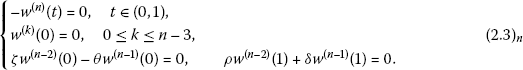
• (e) $0\leq g_{n}(t,s)\leq\frac{L}{(n-2)!} G(s,s)$ for $(t,s)\in [0,1]\times[0,1]$.

3 Eigenvalue characterization

Recall that $E=\{\lambda>0 \mid \mbox{(1.1) has a positive solution}\}$. In this section, we shall establish criteria for E to contain an interval (Theorem 3.5), and for E to be an interval (Corollary 3.7), which may either be bounded or unbounded (Theorem 3.9).

To begin, we consider the initial value problem

$$ \left \{ \begin{array}{@{}l} y^{(q)}(t)=x(t),\quad t\in(0,1),\\ y(0)=y'(0)=y''(0)=\cdots=y^{(q-1)}(0)=0. \end{array} \right . $$

(3.1)

Noting the initial conditions in (3.1), we have by repeated integration

$$ y^{(k)}(t)=\int_{0}^{t}\int _{0}^{s_{1}}\int_{0}^{s_{2}} \cdots\int_{0}^{s_{q-k-1}}x (s_{q-k} )\,ds_{q-k}\cdots \,ds_{1},\quad 0\leq k\leq q-1. $$

(3.2)

Denote the integral

$$ J^{k}x(t)=\int_{0}^{t}\int _{0}^{s_{1}}\int_{0}^{s_{2}} \cdots\int_{0}^{s_{k-1}}x (s_{k} )\,ds_{k}\cdots \,ds_{1},\quad k\geq1. $$

(3.3)

Then (3.2) is simply

$$ y^{(k)}(t)= J^{q-k}x(t),\quad 0\leq k\leq q-1. $$

(3.4)

In view of (3.1) and (3.4), we can rewrite (1.1) as the following $(m-q)$ th order Sturm-Liouville boundary value problem:

$$ \left \{ \begin{array}{@{}l} x^{(m-q)}(t)+\lambda F (t,\tilde{J}x(t))=0,\quad t\in(0,1), \\ x^{(k)}(0)=0,\quad 0\leq k\leq m-q-3, \\ \zeta x^{(m-q-2)}(0)-\theta x^{(m-q-1)}(0)=0,\qquad \rho x^{(m-q-2)}(1)+\delta x^{(m-q-1)}(1)=0, \end{array} \right . $$

(3.5)

where we denote

$$\tilde{J}x(t)= \bigl(J^{q}x(t),J^{q-1}x(t),\ldots,Jx(t),x(t) \bigr). $$

If (3.5) has a solution $x^{*}$, then the boundary value problem (1.1) has a solution $y^{*}$ given by

$$ y^{*}(t)=J^{q}x^{*}(t)=\int_{0}^{t}\int _{0}^{s_{1}}\int_{0}^{s_{2}} \cdots\int_{0}^{s_{q-1}}x^{*} (s_{q} )\,ds_{q}\cdots \,ds_{1}. $$

(3.6)

Hence, the existence of a solution of (1.1) follows from the existence of a solution of (3.5). Further, it is obvious from (3.6) that $y^{*}$ is positive if $x^{*}$ is. An eigenvalue of (3.5) is thus also an eigenvalue of (1.1), i.e.,

$$E= \bigl\{ \lambda>0 \mid (1.1)\mbox{ has a positive solution} \bigr\} = \bigl\{ \lambda>0 \mid (3.5) \mbox{ has a positive solution} \bigr\} . $$

We shall study the eigenvalue problem (1.1) via (3.5) and a new technique will be developed to handle the nonlinear term F.

For easy reference, the conditions that will be mentioned later are listed below.

• (C1) There exist continuous functions $f:(0,\infty)^{q+1} \to(0,\infty)$ and $a,b:(0,1)\to[0,\infty)$ such that for $t\in(0,1)$ and $u_{j}\in(0,\infty)$, $1\leq j\leq q+1$,

  $$a(t)f(u_{1},\ldots,u_{q+1})\leq F(t,u_{1}, \ldots,u_{q+1})\leq b(t)f(u_{1},\ldots,u_{q+1}). $$

• (C2) $a(t)$ is not identically zero on any nondegenerate subinterval of $(0,1)$ and there exists $r\in (0,1]$ such that $a(t)\geq rb(t)$ for all $t\in(0,1)$.

• (C3) $0<\int_{0}^{1}(\theta+\zeta t)[\delta +\rho(1-t)]b(t)\,dt<\infty$.

• (C4) f is nondecreasing in each of its arguments, i.e., for $u_{j},v,w\in(0,\infty)$, $1\leq j\leq q+1$ with $v\leq w$, we have

  $$f(u_{1},\ldots,u_{i-1},v,u_{i+1}, \ldots,u_{q+1})\leq f(u_{1},\ldots ,u_{i-1},w,u_{i+1}, \ldots,u_{q+1}),\quad 1\leq i\leq q+1. $$

• (C5) For $t\in(0,1)$ and $u_{j},v,w\in(0,\infty)$, $1\leq j\leq q+1$ with $v\leq w$, we have

  $$\begin{aligned} F(t,u_{1},\ldots,u_{i-1},v,u_{i+1}, \ldots,u_{q+1})\leq F(t,u_{1},\ldots ,u_{i-1},w,u_{i+1}, \ldots,u_{q+1}),& \\ 1\leq i\leq q+1.& \end{aligned}$$

Let the Banach space

$$B= \bigl\{ x\in C^{(m-q)}(0,1)\cap C^{(m-q-1)}[0,1] \mid x^{(k)}(0)=0, 0\leq k\leq m-q-3 \bigr\} $$

be equipped with the norm

$$\| x\|=\sup_{t\in[0,1]}\bigl| x^{(m-q-2)}(t)\bigr|. $$

Throughout the paper, let $\eta\in (0,\frac{1}{2} )$ be fixed. Define the cone C in B by

$$ C= \Bigl\{ x\in B \bigm| x^{(m-q-2)}(t)\geq0, t\in [0,1]; \min _{t\in[\eta,1-\eta]} x^{(m-q-2)}(t)\geq\gamma\|x\| \Bigr\} , $$

(3.7)

where $\gamma=rK_{\eta}/L$. For a constant $M>0$, let

$$C(M)=\bigl\{ x\in C \mid \|x\|\leq M\bigr\} . $$

Lemma 3.1

[36, 37]

Let $x\in B$. For $0\leq i\leq m-q-2$, we have

$$ \bigl|x^{(i)}(t)\bigr|\leq\frac{t^{m-q-2-i}}{(m-q-2-i)!} \|x\|,\quad t\in[0,1]. $$

(3.8)

In particular,

$$ \bigl|x(t)\bigr|\leq\frac{1}{(m-q-2)!} \|x\|,\quad t\in[0,1]. $$

(3.9)

Lemma 3.2

[36, 37]

Let $x\in C$. For $0\leq i\leq m-q-2$, we have

$$ x^{(i)}(t)\geq0,\quad t\in[0,1], $$

(3.10)

and

$$ x^{(i)}(t)\geq(t-\eta)^{m-q-2-i}\frac{\gamma}{(m-q-2-i)!} \|x\|,\quad t \in[ \eta,1-\eta]. $$

(3.11)

In particular, we have, for fixed $z\in(\eta,1-\eta)$,

$$ x(t)\geq(z-\eta)^{m-q-2}\frac{\gamma}{(m-q-2)!} \|x\|,\quad t\in [z,1-\eta]. $$

(3.12)

Remark 3.1

If $x^{*}\in C$ is a nontrivial solution of (3.5), then (3.10) and (3.12) imply that $x^{*}$ is a positive solution of (3.5). As noted earlier a positive solution $y^{*}$ of (1.1) can be obtained via (3.6).

The next result is useful in handling the nonlinear term F.

Lemma 3.3

Let $x\in C$ and let $z\in(\eta,1-\eta)$ be fixed. Then we have, for $1\leq k\leq q$,

$$ J^{k} x(t)\leq\frac{1}{(m-q-2)!} \|x\|,\quad t\in[0,1], $$

(3.13)

and

$$ J^{k} x(t)\geq(z-\eta)^{m-q-2+k}\frac{\gamma}{(m-q-2+k)!} \|x\| ,\quad t \in[z,1-\eta]. $$

(3.14)

Proof

Since $x\in C\subset B$, using (3.9) we obtain for $1\leq k\leq q$ and $t\in[0,1]$,

$$\begin{aligned} J^{k}x(t) =& \int_{0}^{t}\int _{0}^{s_{1}}\int_{0}^{s_{2}} \cdots\int_{0}^{s_{k-1}}x (s_{k} )\,ds_{k}\cdots \,ds_{1} \\ \leq& \int_{0}^{1}\int_{0}^{1} \int_{0}^{1}\cdots\int_{0}^{1} \frac{\|x\|}{(m-q-2)!}\,ds_{k}\cdots \,ds_{1} = \frac{\|x\|}{(m-q-2)!}. \end{aligned}$$

Next, since $x\in C$, it follows from (3.11) that

$$ x(t)\geq(t-\eta)^{m-q-2}\frac{\gamma\|x\|}{(m-q-2)!},\quad t\in[\eta,1-\eta]. $$

(3.15)

Let $t\in[z,1-\eta]$. Using (3.15) we find, for $1\leq k\leq q$,

$$\begin{aligned} J^{k} x(t) =&\int_{0}^{t}\int _{0}^{s_{1}}\int_{0}^{s_{2}} \cdots\int_{0}^{s_{k-1}}x (s_{k} )\,ds_{k}\cdots \,ds_{1} \geq\int_{\eta}^{z}\int_{\eta}^{s_{1}} \int_{\eta}^{s_{2}}\cdots\int_{\eta}^{s_{k-1}}x (s_{k} )\,ds_{k}\cdots \,ds_{1} \\ \geq&\int_{\eta}^{z}\int_{\eta}^{s_{1}} \int_{\eta}^{s_{2}}\cdots\int_{\eta}^{s_{k-1}}(s_{k}- \eta)^{m-q-2} \frac{\gamma\|x\|}{(m-q-2)!}\,ds_{k}\cdots \,ds_{1} \\ =& (z-\eta)^{m-q-2+k}\frac{\gamma\|x\|}{(m-q-2+k)!}. \end{aligned}$$

 □

In view of Remark 3.1, to obtain a positive solution of (3.5), we shall seek a fixed point of the operator S in the cone C, where $S:C\rightarrow B$ is defined by

$$ Sx(t)= \lambda\int_{0}^{1} g_{m-q}(t,s)F \bigl(s,\tilde{J}x(s) \bigr)\,ds,\quad t\in[0,1]. $$

(3.16)

Recall that $g_{m-q}(t,s)$ (see Lemma 2.2(d)) is the Green’s function of ((2.3) _n )$_{m-q}$, thus (3.16) is equivalent to

$$ (Sx)^{(m-q-2)}(t)= \lambda\int_{0}^{1} G(t,s)F \bigl(s,\tilde{J}x(s) \bigr)\,ds,\quad t\in[0,1], $$

(3.17)

where $G(t,s)$ is the Green’s function of (2.1).

We further define the operators $U,V:C\to B$ by

$$Ux(t)=\lambda\int_{0}^{1}g_{m-q}(t,s)a(s)f \bigl(\tilde{J}x(s) \bigr)\,ds \quad\mbox{and}\quad Vx(t)=\lambda\int _{0}^{1}g_{m-q}(t,s)b(s)f \bigl(\tilde{J}x(s) \bigr)\,ds. $$

As in (3.17), differentiating gives

$$(Ux)^{(m-q-2)}(t)=\lambda\int_{0}^{1}G(t,s)a(s)f \bigl(\tilde{J}x(s) \bigr)\,ds $$

and

$$(Vx)^{(m-q-2)}(t)=\lambda\int_{0}^{1}G(t,s)b(s)f \bigl(\tilde{J}x(s) \bigr)\,ds. $$

If (C1) is satisfied, then it is clear that

$$ Ux(t)\leq Sx(t)\leq Vx(t),\quad t\in[0,1], $$

(3.18)

and

$$ (Ux)^{(m-q-2)}(t)\leq(Sx)^{(m-q-2)}(t)\leq(Vx)^{(m-q-2)}(t),\quad t\in [0,1]. $$

(3.19)

Lemma 3.4

Let (C1)-(C4) hold. Then the operator S is compact on the cone C.

Proof

Let us consider the case when $a(t)$ is unbounded in a deleted right neighborhood of 0 and also in a deleted left neighborhood of 1. Clearly, $b(t)$ is also unbounded near 0 and 1. For $n\in\{1,2,3,\ldots\}$, let $a_{n}, b_{n}:[0,1]\to[0,\infty)$ be defined by

$$a_{n}(t)= \left \{ \begin{array}{@{}l@{\quad}l} a ( \frac{1}{n+1} ),& 0\leq t\leq \frac{1}{n+1} ,\\ a(t), & \frac{1}{n+1}\leq t\leq \frac{n}{n+1}, \\ a ( \frac{n}{n+1} ),& \frac{n}{n+1}\leq t\leq1, \end{array} \right . $$

and

$$b_{n}(t)= \left \{ \begin{array}{@{}l@{\quad}l} b ( \frac{1}{n+1} ), & 0\leq t\leq \frac{1}{n+1}, \\ b(t), & \frac{1}{n+1}\leq t\leq \frac{n}{n+1},\\ b ( \frac{n}{n+1} ), & \frac {n}{n+1}\leq t\leq1. \end{array} \right . $$

Also, we define the operators $U_{n},V_{n}:C\to B$ by

$$U_{n}x(t)=\lambda\int_{0}^{1}g_{m-q}(t,s)a_{n}(s)f \bigl(\tilde{J}x(s) \bigr)\,ds $$

and

$$V_{n}x(t)=\lambda\int_{0}^{1}g_{m-q}(t,s)b_{n}(s)f \bigl(\tilde{J}x(s) \bigr)\,ds. $$

It is standard that, for each n, both $U_{n}$ and $V_{n}$ are compact operators on C. Let $M>0$ and $x\in C(M)$. For $t\in [0,1]$, we obtain

$$\begin{aligned} \bigl\vert V_{n}x(t)-Vx(t)\bigr\vert \leq& {\lambda\int _{0}^{1}g_{m-q}(t,s) \bigl|b_{n}(s)-b(s)\bigr|f \bigl(\tilde{J}x(s) \bigr)\,ds} \\ =& \lambda\int_{0}^{\frac{1}{n+1}}g_{m-q}(t,s) \bigl|b_{n}(s)-b(s)\bigr|f \bigl(\tilde{J}x(s) \bigr)\,ds \\ &{} + \lambda\int^{1}_{\frac{n}{n+1}} g_{m-q}(t,s)\bigl|b_{n}(s)-b(s)\bigr|f \bigl(\tilde{J}x(s) \bigr)\,ds \\ =& \lambda\int_{0}^{\frac{1}{n+1}}g_{m-q}(t,s) \biggl\vert b_{n} \biggl(\frac{1}{n+1} \biggr)-b(s)\biggr\vert f \bigl(\tilde{J}x(s) \bigr)\,ds \\ &{} + \lambda\int^{1}_{\frac{n}{n+1}} g_{m-q}(t,s) \biggl\vert b_{n} \biggl(\frac{n}{n+1} \biggr)-b(s)\biggr\vert f \bigl(\tilde{J}x(s) \bigr)\,ds. \end{aligned}$$

Since $\|x\|\leq M$, from (3.13) we get

$$J^{k} x(s)\leq\frac{M}{(m-q-2)!},\quad s\in[0,1], 1\leq k\leq q. $$

Hence, together with (3.9), it follows from the monotonicity of f (condition (C4)) that

$$\begin{aligned} f \bigl(\tilde{J}x(s) \bigr) =& f \bigl(J^{q}x(s),J^{q-1}x(s), \ldots,Jx(s),x(s) \bigr) \\ \leq& f \biggl(\frac{M}{(m-q-2)!},\frac{M}{(m-q-2)!},\ldots, \frac{M}{(m-q-2)!} \biggr) \equiv \bar{f}_{M}. \end{aligned}$$

(3.20)

Applying (3.20) and Lemma 2.2(e), we obtain

$$\begin{aligned} \bigl\vert V_{n}x(t)-Vx(t)\bigr\vert \leq& \lambda\bar{f}_{M} \biggl[\int_{0} ^{\frac{1}{n+1}} \frac{LG(s,s)}{(m-q-2)!}\biggl\vert b \biggl(\frac {1}{n+1} \biggr)-b(s)\biggr\vert \,ds \\ &{}+ \int^{1}_{\frac{n}{n+1}} \frac{LG(s,s)}{(m-q-2)!}\biggl\vert b \biggl(\frac{n}{n+1} \biggr)-b(s)\biggr\vert \,ds \biggr]. \end{aligned}$$

The integrability of $G(s,s)b(s)$ (which is simply (C3)) ensures that $V_{n}$ converges uniformly to V on $C(M)$. Hence, V is compact on C. By a similar argument, we see that $U_{n}$ converges uniformly to U on $C(M)$ and therefore U is also compact on C. It follows immediately from inequality (3.18) that the operator S is compact on C. □

Remark 3.2

From the proof of Lemma 3.4, we see that if the functions a and b are continuous on the close interval $[0,1]$, then the conditions (C3) and (C4) are not needed in Lemma 3.4.

The first main result shows that E contains an interval.

Theorem 3.5

Let (C1)-(C4) hold. Then there exists $\ell>0$ such that the interval $(0,\ell] \subseteq E$.

Proof

For a given $M>0$, we define

$$ \ell=M \biggl[\bar{f}_{M} L\int_{0}^{1}G(s,s)b(s)\,ds \biggr]^{-1}. $$

(3.21)

Let $\lambda\in(0, \ell]$. We shall prove that $S (C(M))\subseteq C(M)$. For this, let $x\in C(M)$. First, we shall show that $Sx\in C$. From (3.19), it is clear that

$$ (Sx)^{(m-q-2)}(t)\geq\lambda\int_{0}^{1}G(t,s)a(s) f \bigl(\tilde{J}x(s) \bigr)\,ds\geq0,\quad t\in[0,1]. $$

(3.22)

Also, (3.19) and Lemma 2.2(b) provide

$$(Sx)^{(m-q-2)}(t) \leq\lambda\int_{0}^{1}G(t,s)b(s) f \bigl(\tilde{J}x(s) \bigr)\,ds \leq \lambda\int_{0}^{1}LG(s,s) b(s)f \bigl( \tilde{J}x(s) \bigr)\,ds,\quad t\in[0,1], $$

which immediately implies

$$ \|Sx\|\leq\lambda\int_{0}^{1}LG(s,s) b(s)f \bigl(\tilde{J}x(s) \bigr)\,ds. $$

(3.23)

Further, using (3.19), Lemma 2.2(c), (C2), and (3.23) successively, we find, for $t\in [\eta,1-\eta]$,

$$\begin{aligned} (Sx)^{(m-q-2)}(t) \geq& \lambda\int_{0}^{1}G(t,s)a(s)f \bigl(\tilde{J}x(s) \bigr)\,ds \\ \geq& {\lambda\int_{0}^{1}K_{\eta}G(s,s)a(s) f \bigl(\tilde{J}x(s) \bigr)\,ds} \\ \geq& {\lambda\int_{0}^{1}K_{\eta}G(s,s) rb(s) f \bigl(\tilde{J}x(s) \bigr)\,ds} \\ \geq& \frac{K_{\eta}}{L} r\|Sx\| = \gamma\|Sx\|. \end{aligned}$$

Hence,

$$ \min_{t\in[\eta,1-\eta]} (Sx)^{(m-q-2)}(t)\geq\gamma\| Sx\|. $$

(3.24)

Inequalities (3.22) and (3.24) show that $Sx\in C$.

Next, we shall prove that $\|Sx\|\leq M$. Noting that $\|x\|\leq M$, we use (3.20), Lemma 2.2(b), and (3.21) to get

$$\begin{aligned} (Sx)^{(m-q-2)}(t) \leq& \ell \int_{0}^{1}G(t,s)b(s) f \bigl(\tilde{J}x(s) \bigr)\,ds \\ \leq& {\ell\bar{f}_{M}\int_{0}^{1} LG(s,s)b(s)\,ds} = M, \quad t\in[0,1], \end{aligned}$$

or equivalently

$$\|Sx\|\leq M. $$

Hence, $S(C(M))\subseteq C(M)$. Also, the standard arguments yield that S is completely continuous. By Schauder’s fixed point theorem, S has a fixed point in $C(M)$. Clearly, this fixed point is a positive solution of (3.5) and therefore λ is an eigenvalue of (3.5). Noting that $\lambda\in(0, \ell]$ is arbitrary, it follows immediately that the interval $(0,\ell] \subseteq E$. □

Remark 3.3

From the proof of Theorem 3.5, it is clear that conditions (C1) and (C2) ensure that $S:C\to C$.

Theorem 3.6

Let (C1)-(C5) hold. Suppose that $\lambda^{*}\in E$. For any $\lambda\in(0,\lambda^{*})$, we have $\lambda\in E$, i.e., $(0,\lambda^{*}]\subseteq E$.

Proof

Let $x^{*}$ be the eigenfunction corresponding to the eigenvalue $\lambda^{*}$. Then we have

$$ x^{*}(t)= Sx^{*}(t) = \lambda^{*}\int_{0}^{1} g_{m-q}(t,s)F \bigl(s,\tilde{J}x^{*}(s) \bigr)\,ds,\quad t\in[0,1]. $$

(3.25)

Define

$$A= \bigl\{ x\in B \mid 0\leq x(t)\leq x^{*}(t), t\in[0,1] \bigr\} . $$

Let $\lambda\in (0,\lambda^{*})$ and $x\in A$. It is obvious from definition (3.3) that

$$J^{k}x(t)\leq J^{k}x^{*}(t),\quad t\in[0,1], 1\leq k\leq q. $$

Now, applying (C5) and noting (3.25), we obtain

$$\begin{aligned} 0 \leq& Sx(t)= \lambda\int_{0}^{1} g_{m-q}(t,s)F \bigl(s,\tilde{J}x(s) \bigr)\,ds \\ \leq&\lambda^{*}\int_{0}^{1} g_{m-q}(t,s)F \bigl(s,\tilde{J}x^{*}(s) \bigr)\,ds \\ =& Sx^{*}(t),\quad t\in[0,1]. \end{aligned}$$

This shows that the operator S maps A into A. Moreover, the operator S is continuous and completely continuous. Schauder’s fixed point theorem guarantees that S has a fixed point in A which is a positive solution of (3.5). Hence, λ is an eigenvalue of (3.5), i.e., $\lambda\in E$. □

The next result states that E is itself an interval.

Corollary 3.7

Let (C1)-(C5) hold. If $E\neq\emptyset$, then E is an interval.

Proof

Suppose E is not an interval. Then there exist $\lambda_{0}, \lambda_{1}\in E$ ($\lambda_{0}<\lambda_{1}$), and $\tau\in (\lambda_{0}, \lambda_{1})$ with $\tau\notin E$. However, this is not possible as Theorem 3.6 guarantees that $\tau\in E$. Hence, E is an interval. □

The next result gives upper and lower bounds of an eigenvalue.

Theorem 3.8

Let (C1)-(C4) hold. Let λ be an eigenvalue of (3.5) and $x\in C$ be a corresponding eigenfunction. Further, let $\|x\|=p$ and $z\in(\eta,1-\eta)$ be fixed. Then

$$ \lambda\geq\frac{p}{f (\frac{p}{(m-q-2)!},\frac {p}{(m-q-2)!},\ldots,\frac{p}{(m-q-2)!} )} \biggl[\int_{0}^{1} LG(s,s)b(s)\,ds \biggr]^{-1}, $$

(3.26)

and

$$\begin{aligned} \lambda\leq{}&\frac{p}{f (\frac{\gamma p}{(m-2)!}(z-\eta)^{m-2},\frac{\gamma p}{(m-3)!}(z-\eta)^{m-3},\ldots,\frac{\gamma p}{(m-q-1)!}(z-\eta)^{m-q-1},\frac{\gamma p}{(m-q-2)!}(z-\eta)^{m-q-2} )} \\ &{}\times \biggl[\int _{z}^{1-\eta} G(t_{0},s)a(s)\,ds \biggr]^{-1}, \end{aligned}$$

(3.27)

where $t_{0}$ is any number in $(0,1)$ such that $x^{(m-q-2)}(t_{0})\neq0$.

Proof

Let $t_{1}\in[0,1]$ be such that

$$p=\|x\|=x^{(m-q-2)}(t_{1}). $$

Then, applying (3.19), Lemma 2.2(b), (3.20), and (C4), we find

$$\begin{aligned} p =& x^{(m-q-2)}(t_{1})= (Sx)^{(m-q-2)}(t_{1}) \\ \leq& \lambda \int_{0}^{1}G(t_{1},s)b(s)f \bigl(\tilde{J}x(s) \bigr)\,ds \\ \leq& {\lambda\int_{0}^{1}LG(s,s) b(s) \bar{f}_{p} \,ds,} \end{aligned}$$

which gives (3.26) immediately.

Next, noting (3.19), (3.14), (3.12), and (C4), we get

$$\begin{aligned} p \geq& x^{(m-q-2)}(t_{0}) \\ \geq& \lambda {\int_{0}^{1}G(t_{0},s)a(s) f \bigl(\tilde{J}x(s) \bigr)\,ds} \\ \geq& \lambda {\int_{z}^{1-\eta} G(t_{0},s)a(s) f \bigl(\tilde{J}x(s) \bigr)\,ds} \\ \geq& \lambda{ \int_{z}^{1-\eta}} G(t_{0},s)a(s)\,ds \\ &{} \times f \biggl(\frac{\gamma p}{(m-2)!}(z-\eta)^{m-2}, \frac {\gamma p}{(m-3)!}(z-\eta)^{m-3},\ldots,\frac{\gamma p}{(m-q-1)!}(z- \eta)^{m-q-1},\\ &{}\frac{\gamma p}{(m-q-2)!}(z-\eta)^{m-q-2} \biggr), \end{aligned}$$

from which (3.27) is immediate. □

The next result gives the criteria for E to be a bounded/unbounded interval.

Theorem 3.9

Define

$$\begin{aligned}& P_{B}= \biggl\{ f \Bigm| \frac {u}{f(u,u,\ldots,u)} \textit{ is bounded for }u\in(0, \infty) \biggr\} , \\& P_{0}= \biggl\{ f \Bigm| {\lim_{u\to\infty}\frac{u}{ f(u,u,\ldots,u)}=0} \biggr\} , \\& P_{\infty}= \biggl\{ f \Bigm| {\lim_{u\to\infty }\frac{u}{ f(u,u,\ldots,u)}= \infty} \biggr\} . \end{aligned}$$

• (a) Let (C1)-(C5) hold. If $f\in P_{B}$, then $E=(0,\ell)$ or $(0,\ell]$ for some $\ell\in(0, \infty)$.

• (b) Let (C1)-(C5) hold. If $f\in P_{0}$, then $E=(0,\ell]$ for some $\ell\in(0,\infty)$.

• (c) Let (C1)-(C4) hold. If $f\in P_{\infty}$, then $E=(0,\infty)$.

Proof

(a) This follows from (3.27) and Corollary 3.7.

(b) Since $P_{0}\subseteq P_{B}$, we have from Case (a) that $E= (0,\ell)$ or $(0,\ell]$ for some $\ell\in(0,\infty)$. In particular,

$$\ell=\sup E. $$

Let $\{\lambda_{n}\}_{n=1}^{\infty}$ be a monotonically increasing sequence in E which converges to ℓ, and let $\{x_{n}\}_{n=1}^{\infty}$ be a corresponding sequence of eigenfunctions in the context of (3.5). Further, let $p_{n}= \| x_{n}\|$. Then (3.27) together with $f\in P_{0}$ implies that no subsequence of $\{p_{n}\}_{n=1}^{\infty}$ can diverge to infinity. Thus, there exists $M>0$ such that $p_{n}\leq M$ for all n. So $\{x_{n}\}_{n=1}^{\infty}$ is uniformly bounded. This implies that there is a subsequence of $\{x_{n}\}_{n=1}^{\infty}$, relabeled as the original sequence, which converges uniformly to some x, where $x(t) \geq0$ for $t\in[0,1]$. Clearly, we have $Sx_{n}=x_{n}$, i.e.,

$$ x_{n}(t)=\lambda_{n}\int_{0}^{1} g_{m-q}(t,s)F \bigl(s,\tilde{J}x_{n}(s) \bigr)\,ds,\quad t \in[0,1]. $$

(3.28)

Since $x_{n}$ converges to x and $\lambda_{n}$ converges to ℓ, letting $n\to\infty$ in (3.28) leads to

$$x(t)=\ell\int_{0}^{1} g_{m-q}(t,s)F \bigl(s,\tilde{J}x(s) \bigr)\,ds,\quad t\in[0,1]. $$

Hence, ℓ is an eigenvalue with corresponding eigenfunction x, i.e., $\ell=\sup E\in E$. This completes the proof for Case (b).

(c) Let $\lambda>0$ be fixed. Choose $\epsilon>0$ so that

$$ \lambda \frac{L}{(m-q-2)!}\int_{0}^{1} G(s,s)b(s)\,ds\leq\frac {1}{\epsilon}. $$

(3.29)

If $f\in P_{\infty}$, then there exists $M=M(\epsilon)>0$ such that

$$ f(u,u,\ldots,u)<\epsilon u, \quad u\geq\frac{M}{(m-q-2)!}. $$

(3.30)

We shall show that $S(C(M))\subseteq C(M)$. Let $x\in C(M)$. From the proof of Theorem 3.5, we have (3.22) and (3.24) and so $Sx\in C$. It remains to show that $\|Sx\|\leq M$. Applying (3.19), Lemma 2.2(b), (3.20), (3.30), and (3.29), we find, for $t\in[0,1]$,

$$\begin{aligned} (Sx)^{(m-q-2)}(t) \leq& \lambda \int_{0}^{1}G(t,s)b(s)f \bigl(\tilde{J}x(s) \bigr)\,ds \\ \leq& {\lambda\int_{0}^{1}LG(s,s)b(s) f \biggl( \frac{M}{(m-q-2)!},\frac{M}{(m-q-2)!},\ldots, \frac{M}{(m-q-2)!} \biggr)\,ds} \\ \leq& {\lambda\epsilon \frac{M}{(m-q-2)!}\int_{0}^{1} LG(s,s)b(s)\,ds} \leq M. \end{aligned}$$

It follows that $\|Sx\|\leq M$ and hence $S(C(M))\subseteq C(M)$. Also, S is continuous and completely continuous. Schauder’s fixed point theorem guarantees that S has a fixed point in $C(M)$. Clearly, this fixed point is a positive solution of (3.5) and therefore λ is an eigenvalue of (3.5). Since $\lambda>0$ is arbitrary, it shows that $E=(0,\infty)$. □

Example 3.1

Consider the Sturm-Liouville boundary value problem

$$ \left \{ \begin{array}{@{}l} y^{(5)}(t)+\lambda F (t,y(t),y'(t),y''(t),y'''(t) )=0, \quad t\in(0,1),\\ y(0)=y'(0)=y''(0)=0,\qquad 2y^{(3)}(0)-y^{(4)}(0)=0,\qquad -y^{(3)}(1)+3y^{(4)}(1)=0, \end{array} \right . $$

(3.31)

where $\lambda>0$ and

$$\begin{aligned} F\bigl(t,y,y',y'',y''' \bigr) =& \biggl[\frac{300+900t+270t^{2}+90t^{3}+10t^{4}-3t^{5}}{200}+2 \biggr]^{-1/2} \\ &{}\times \biggl(\frac{y+y'+y''+y'''}{4} +2 \biggr)^{1/2}. \end{aligned}$$

Here, $m=5$, $q=3$, $\zeta=2$, $\theta=1$, $\rho=-1$, and $\delta=3$. Clearly, (C1)-(C5) are satisfied with

$$a(t)=b(t)= \biggl[\frac{300+900t+270t^{2}+90t^{3}+10t^{4}-3t^{5}}{200}+2 \biggr]^{-1/2} $$

and

$$f(u_{1},u_{2},u_{3}, u_{4})= \biggl( \frac{u_{1}+u_{2}+u_{3}+u_{4}}{4}+2 \biggr)^{1/2}. $$

It is obvious that $f\in P_{\infty}$. Hence, by Theorem 3.9(c) we have $E=(0,\infty)$. In fact, when $\lambda=\frac{36}{5}\in(0,\infty)$, (3.31) has a positive solution $y(t)=t^{3}+\frac{1}{2}t^{4}-\frac{3}{50}t^{5}$.

4 Explicit eigenvalue intervals

In this section, the functions a and b appearing in (C1)-(C3) are assumed to be continuous on the closed interval $[0,1]$. Hence, noting Remark 3.2, we shall not require conditions (C3) and (C4) to show the compactness of the operator S. With respect to the function f in (C1), we define

$$\begin{aligned}& \overline{f}_{0}=\limsup_{u_{i}\to0, 1\leq i\leq q+1} \frac{f(u_{1},u_{2},\ldots,u_{q+1})}{u_{q+1}}, \qquad \underline{f}_{0}=\liminf_{u_{i}\to0, 1\leq i\leq q+1} \frac{f(u_{1},u_{2},\ldots,u_{q+1})}{u_{q+1}}, \\& \overline{f}_{\infty}=\limsup_{u_{i}\to\infty, 1\leq i\leq q+1} \frac{f(u_{1},u_{2},\ldots,u_{q+1})}{u_{q+1}}, \qquad \underline{f}_{\infty}=\liminf_{u_{i}\to\infty, 1\leq i\leq q+1} \frac{f(u_{1},u_{2},\ldots,u_{q+1})}{u_{q+1}}. \end{aligned}$$

Our main tool in this section is the Krasnosel’skii fixed point theorem in a cone (Theorem 2.1) which we shall apply with the operator S and the cone C defined in (3.16) and (3.7), respectively. Recall that $\eta\in (0,\frac{1}{2} )$ is fixed. Throughout this section, we further let $z\in[\eta,1-\eta]$ be fixed. Define $t_{z}, t^{*}\in[0,1]$ by

$$ \begin{aligned} &\int_{z}^{1-\eta}G(t_{z},s)a(s) (s-\eta )^{m-q-2}\,ds=\sup_{t\in[0,1]} \int_{z}^{1-\eta}G(t,s)a(s) (s-\eta)^{m-q-2}\,ds, \\ &\int_{\eta}^{1-\eta}G\bigl(t^{*},s\bigr)a(s) (s- \eta)^{m-q-2}\,ds=\sup_{t\in [0,1]} \int_{\eta}^{1-\eta}G(t,s)a(s) (s-\eta)^{m-q-2}\,ds. \end{aligned} $$

(4.1)

Theorem 4.1

Let (C1)-(C3) hold. Then $\lambda\in E$ if λ satisfies

$$\begin{aligned} &\frac{1}{\underline{f}_{\infty}} \biggl[\frac{\gamma}{(m-q-2)!}\int_{z}^{1-\eta} G(t_{z},s)a(s) (s-\eta)^{m-q-2}\,ds \biggr]^{-1} \\ &\quad< \lambda<\frac {1}{\overline{f}_{0}} \biggl[\frac{L}{(m-q-2)!}\int_{0}^{1}G(s,s)b(s)s^{m-q-2}\,ds \biggr]^{-1}. \end{aligned}$$

(4.2)

Proof

Let λ satisfy (4.2) and let $\epsilon >0$ be such that

$$\begin{aligned} &\frac{1}{\underline{f}_{\infty}-\epsilon} \biggl[\frac{\gamma }{(m-q-2)!}\int_{z}^{1-\eta} G(t_{z},s)a(s) (s-\eta)^{m-q-2}\,ds \biggr]^{-1} \\ &\quad< \lambda<\frac {1}{\overline{f}_{0}+\epsilon} \biggl[\frac{L}{(m-q-2)!}\int_{0}^{1}G(s,s)b(s)s^{m-q-2}\,ds \biggr]^{-1}. \end{aligned}$$

(4.3)

First, we choose $w>0$ so that

$$ f(u_{1},u_{2},\ldots,u_{q+1})\leq(\overline{f}_{0}+\epsilon) u_{q+1},\quad 0< u_{i}\leq w,\ 1\leq i \leq q+1. $$

(4.4)

Let $x\in C$ be such that $\|x\|=w(m-q-2)!$. By (3.13) and (3.9), we get

$$ \left \{ \begin{array}{@{}l }x(s)\leq\frac{\|x\|}{(m-q-2)!}=w, \quad s\in [0,1],\\ J^{k} x(s)\leq \frac{\|x\|}{(m-q-2)!}=w,\quad s\in[0,1],\ 1\leq k\leq q. \end{array} \right . $$

(4.5)

Thus, together with (3.19), Lemma 2.2(b), (4.5), (4.4), (3.8), and (4.3), we find, for $t\in[0,1]$,

$$\begin{aligned} (Sx)^{(m-q-2)}(t) \leq& \lambda\int_{0}^{1}LG(s,s)b(s)f \bigl(\tilde{J}x(s) \bigr)\,ds \\ \leq& \lambda \int_{0}^{1}LG(s,s)b(s) ( \overline{f}_{0}+\epsilon)x(s)\,ds \\ \leq& \lambda\int_{0}^{1}LG(s,s)b(s) (\overline{f}_{0}+\epsilon)\frac{s^{m-q-2}}{(m-q-2)!} \|x\|\,ds \leq \|x\|. \end{aligned}$$

It follows that

$$ \|Sx\|\leq\|x\|. $$

(4.6)

If we set $\Omega_{1}=\{x\in B \mid \|x\|< w(m-q-2)!\}$, then (4.6) holds for $x\in C\cap\partial\Omega_{1}$.

Next, let $d>0$ be such that

$$ f(u_{1},u_{2},\ldots,u_{q+1})\geq(\underline{f}_{\infty}-\epsilon) u_{q+1},\quad u_{i}\geq d,\ 1\leq i \leq q+1. $$

(4.7)

Let $x\in C$ be such that

$$\begin{aligned} \|x\| =&\max \biggl\{ w(m-q-2)!+1,\ \frac {d(m-q-2)!}{\gamma(z-\eta)^{m-q-2}},\ \frac{d(m-q-2+k)!}{\gamma(z-\eta)^{m-q-2+k}},\ 1\leq k\leq q\biggr\} \\ =&\max \biggl\{ w(m-q-2)!+1,\ \frac{d(m-2)!}{\gamma(z-\eta )^{m-2}} \biggr\} \equiv D. \end{aligned}$$

(4.8)

Using (3.12), (3.14), and (4.8), we have

$$ \left \{ \begin{array}{@{}l} x(s)\geq\frac{(z-\eta)^{m-q-2}}{(m-q-2)!} \gamma \|x\|\geq d,\quad s\in[z, 1-\eta],\\ J^{k}x(s)\geq \frac{(z-\eta)^{m-q-2+k}}{(m-q-2+k)!} \gamma\|x\|\geq d, \quad s\in [z,1-\eta],\ 1\leq k\leq q. \end{array} \right . $$

(4.9)

Now, applying (3.19), (4.9), (4.7), and (3.11), we find, for $t\in [0,1]$,

$$\begin{aligned} (Sx)^{(m-q-2)}(t) \geq& \lambda {\int_{z}^{1-\eta} G(t,s)a(s) f \bigl(\tilde{J}x(s) \bigr)\,ds} \\ \geq& \lambda \int_{z}^{1-\eta} G(t,s)a(s) ( \underline{f}_{\infty}-\epsilon)x(s)\,ds \\ \geq& \lambda \int_{z}^{1-\eta} G(t,s)a(s) ( \underline{f}_{\infty}-\epsilon) (s-\eta)^{m-q-2}\frac{\gamma \|x\|}{(m-q-2)!}\,ds. \end{aligned}$$

Taking the supremum on both sides leads to

$$\|Sx\|\geq\lambda\int_{z}^{1-\eta} G(t_{z},s)a(s) (s-\eta)^{m-q-2}\,ds\cdot(\underline{f}_{\infty}-\epsilon)\frac{\gamma\|x\|}{(m-q-2)!}\geq\|x\|, $$

where $t_{z}$ is defined in (4.1), and (4.3) has been used in the last inequality. If we set $\Omega_{2}=\{x\in B \mid \|x\|< D\}$, then for $x\in C\cap \partial\Omega_{2}$ we have

$$ \|Sx\|\geq\|x\|. $$

(4.10)

With (4.6) and (4.10) established and also noting that S maps C into C (Remark 3.3), by Theorem 2.1 S has a fixed point $x\in C\cap(\bar{\Omega}_{2}\backslash\Omega_{1})$ such that $w(m-q-2)!\leq \|x\|\leq D$. Obviously, this x is a positive solution of (3.5) and hence $\lambda\in E$. □

Theorem 4.2

Let (C1)-(C3) hold. Then $\lambda\in E$ if λ satisfies

$$\begin{aligned} &\frac{1}{\underline{f}_{0}} \biggl[\frac{\gamma}{(m-q-2)!}\int_{\eta}^{1-\eta} G \bigl(t^{*},s \bigr)a(s) (s-\eta)^{m-q-2}\,ds \biggr]^{-1} \\ &\quad< \lambda< \frac {1}{\overline{f}_{\infty}} \biggl[\frac{L}{(m-q-2)!}\int_{0}^{1}G(s,s)b(s)\,ds \biggr]^{-1}. \end{aligned}$$

(4.11)

Proof

Let λ satisfy (4.11) and let $\epsilon>0$ be such that

$$\begin{aligned} &\frac{1}{\underline{f}_{0}-\epsilon} \biggl[\frac{\gamma }{(m-q-2)!}\int_{\eta}^{1-\eta} G \bigl(t^{*},s \bigr)a(s) (s-\eta)^{m-q-2}\,ds \biggr]^{-1} \\ &\quad< \lambda< \frac {1}{\overline{f}_{\infty}+\epsilon} \biggl[\frac{L}{(m-q-2)!}\int_{0}^{1}G(s,s)b(s)\,ds \biggr]^{-1}. \end{aligned}$$

(4.12)

First, we pick $w>0$ so that

$$ f(u_{1},u_{2},\ldots,u_{q+1})\geq(\underline{f}_{0}-\epsilon)u_{q+1},\quad 0< u_{i}\leq w,\ 1\leq i\leq q+1. $$

(4.13)

Let $x\in C$ be such that $\|x\|=w(m-q-2)!$. As in (4.5), we have $x(s)\leq w$ and $J^{k}x(s)\leq w$, $1\leq k\leq q$ for $s\in[0,1]$. Hence, applying (3.19), (4.13), and (3.11), we find, for $t\in[0,1]$,

$$\begin{aligned}[b] (Sx)^{(m-q-2)}(t) &\geq {\lambda\int_{0}^{1}G(t,s)a(s) f \bigl(\tilde{J}x(s) \bigr)\,ds} \geq {\lambda\int_{0}^{1}G(t,s) a(s) ( \underline{f}_{0}-\epsilon) x(s)\,ds} \\ &\geq {\lambda\int_{\eta}^{1-\eta}G(t,s) a(s) ( \underline{f}_{0}-\epsilon) (s-\eta)^{m-q-2}\frac{\gamma\|x\|}{(m-q-2)!}\,ds.} \end{aligned} $$

Taking the supremum on both sides and using (4.12) lead to

$$\|Sx\|\geq\lambda\int_{\eta}^{1-\eta}G \bigl(t^{*},s \bigr) a(s) (s-\eta)^{m-q-2}\,ds\cdot(\underline{f}_{0}-\epsilon) \frac{\gamma\|x\|}{(m-q-2)!}\geq\|x\|, $$

where $t^{*}$ is defined in (4.1). Hence, if we set $\Omega_{1}=\{x\in B \mid \|x\| < w(m-q-2)!\}$, then $\|Sx\|\geq\|x\|$ holds for $x\in C\cap\partial\Omega_{1}$.

Next, let $d>0$ be such that

$$ f(u_{1},u_{2},\ldots,u_{q+1})\leq(\overline{f}_{\infty}+\epsilon) u_{q+1}, \quad u_{i}\geq d,\ 1\leq i\leq q+1. $$

(4.14)

We shall consider two cases - when f is bounded and when f is unbounded.

Case 1. Suppose that f is bounded. Then there exists a positive constant M such that

$$ f(u_{1},u_{2},\ldots,u_{q+1})\leq M,\quad u_{i}\in(0,\infty),\ 1\leq i\leq q+1. $$

(4.15)

Let

$$D=\max \biggl\{ w+1, \frac{\lambda M}{(m-q-2)!} \int_{0}^{1}LG(s,s)b(s)\,ds \biggr\} $$

and let $x\in C$ be such that $\|x\|= D(m-q-2)!$. Using (3.19), Lemma 2.2(b), and (4.15), we have, for $t\in[0,1]$,

$$\begin{aligned} (Sx)^{(m-q-2)}(t) \leq& \lambda \int_{0}^{1}LG(s,s)b(s)f \bigl(\tilde{J}x(s) \bigr)\,ds \\ \leq& \lambda \int_{0}^{1}LG(s,s)b(s)M \,ds \leq D(m-q-2)! = \|x\|. \end{aligned}$$

Hence, $\|Sx\|\leq\|x\|$ holds.

Case 2. Suppose that f is unbounded. Then there exists $D>\max \{w+1, d \}$ such that

$$ f(u_{1},u_{2},\ldots,u_{q+1})\leq f(D, D,\ldots,D), \quad 0< u_{i}\leq D,\ 1\leq i\leq q+1. $$

(4.16)

Let $x\in C$ be such that $\|x\|=D(m-q-2)!$. As in (4.5), we have $x(s)\leq D$ and $J^{k}x(s)\leq D$, $1\leq k\leq q$ for $s\in[0,1]$. Now, using (3.19), Lemma 2.2(b), (4.16), (4.14), and (4.12), we get, for $t\in[0,1]$,

$$\begin{aligned} (Sx)^{(m-q-2)}(t) \leq& \lambda \int_{0}^{1}LG(s,s)b(s)f \bigl(\tilde{J}x(s) \bigr)\,ds \\ \leq& \lambda \int_{0}^{1}LG(s,s)b(s)f(D, D, \ldots,D)\,ds \\ \leq& \lambda \int_{0}^{1}LG(s,s) b(s) ( \overline{f}_{\infty}+\epsilon)D \,ds \\ = & \lambda \int_{0}^{1}LG(s,s)b(s) (\overline{f}_{\infty}+\epsilon)\frac{\|x\|}{(m-q-2)!}\,ds \leq \|x\|. \end{aligned}$$

Hence, immediately we have $\|Sx\|\leq\|x\|$.

In both Case 1 and 2, if we set $\Omega_{2}= \{x\in B \mid \|x\|< D(m-q-2)! \}$, then $\|Sx\|\leq\|x\|$ holds for $x\in C\cap\partial\Omega_{2}$.

With (4.6) and (4.10) established and also noting that S maps C into C (Remark 3.3), it follows from Theorem 2.1 that S has a fixed point $x\in C\cap(\bar{\Omega}_{2}\backslash\Omega_{1})$ such that $w(m-q-2)!\leq\|x\|\leq D(m-q-2)!$. Clearly, this x is a positive solution of (3.5) and hence $\lambda\in E$. □

Theorems 4.1 and 4.2 provide explicit eigenvalue intervals as follows.

Corollary 4.3

Let (C1)-(C3) hold. Then

$$\begin{aligned} E \supseteq& \biggl( \frac{1}{\underline{f}_{\infty}} \biggl[\frac{\gamma}{(m-q-2)!}\int _{z}^{1-\eta} G(t_{z},s)a(s) (s- \eta)^{m-q-2}\,ds \biggr]^{-1}, \\ &{}\frac{1}{\overline{f}_{0}} \biggl[ \frac{L}{(m-q-2)!}\int_{0}^{1}G(s,s)b(s)s^{m-q-2}\,ds \biggr]^{-1} \biggr) \\ \supseteq& \biggl( \frac{1}{\underline{f}_{\infty}} \biggl[\frac{\gamma}{(m-q-2)!}\int _{z}^{1-\eta} K_{\eta}G(s,s)a(s) (s- \eta)^{m-q-2}\,ds \biggr]^{-1}, \\ &{}\frac{1}{\overline{f}_{0}} \biggl[ \frac{L}{(m-q-2)!}\int_{0}^{1}G(s,s)b(s)s^{m-q-2}\,ds \biggr]^{-1} \biggr) \end{aligned}$$

and

$$\begin{aligned} E \supseteq& \biggl( \frac{1}{\underline{f}_{0}} \biggl[\frac{\gamma}{(m-q-2)!}\int _{\eta}^{1-\eta} G\bigl(t^{*},s\bigr)a(s) (s- \eta)^{m-q-2}\,ds \biggr]^{-1},\\ &{} \frac{1}{\overline{f}_{\infty}} \biggl[ \frac{L}{(m-q-2)!}\int_{0}^{1}G(s,s)b(s)\,ds \biggr]^{-1} \biggr) \\ \supseteq& \biggl( \frac{1}{\underline{f}_{0}} \biggl[\frac{\gamma}{(m-q-2)!}\int _{\eta}^{1-\eta} K_{\eta}G(s,s)a(s) (s- \eta)^{m-q-2}\,ds \biggr]^{-1},\\ &{} \frac{1}{\overline{f}_{\infty}} \biggl[ \frac{L}{(m-q-2)!}\int_{0}^{1}G(s,s)b(s)\,ds \biggr]^{-1} \biggr). \end{aligned}$$

Proof

We apply Theorems 4.1 and 4.2. Moreover, using Lemma 2.2(c) we have

$$\begin{aligned} \int_{z}^{1-\eta}G(t_{z},s)a(s) (s-\eta )^{m-q-2}\,ds \geq& \sup_{t\in[\eta, 1-\eta]}\int_{z}^{1-\eta}G(t,s)a(s) (s-\eta)^{m-q-2}\,ds \\ \geq& \int_{z}^{1-\eta}K_{\eta}G(s,s)a(s) (s-\eta)^{m-q-2}\,ds \end{aligned}$$

and

$$\begin{aligned} \int_{\eta}^{1-\eta}G\bigl(t^{*},s\bigr)a(s) (s-\eta )^{m-q-2}\,ds \geq& \sup_{t\in[\eta,1-\eta]}\int_{\eta }^{1-\eta}G(t,s)a(s) (s-\eta)^{m-q-2}\,ds \\ \geq& \int_{\eta}^{1-\eta}K_{\eta}G(s,s)a(s) (s-\eta)^{m-q-2}\,ds, \end{aligned}$$

from which we are able to avoid the calculations of $t_{z}$ and $t^{*}$, amid getting smaller intervals. □

The function f is said to be superlinear if $\overline{f}_{0}=0$ and $\underline{f}_{\infty}=\infty$; and f is said to be sublinear if $\underline{f}_{0}=\infty$ and $\overline{f}_{\infty}=0$. The next result is immediate from Corollary 4.3.

Corollary 4.4

Let (C1)-(C3) hold. If f is superlinear or sublinear, then $E=(0,\infty)$, i.e., the boundary value problem (3.5) (or (1.1)) has a positive solution for any $\lambda>0$.

Example 4.1

Consider the Sturm-Liouville boundary value problem

$$ \left \{ \begin{array}{@{}l} y^{(4)}(t)+\lambda F (t,y(t),y'(t),y''(t) )=0,\quad t\in(0,1), \\ y(0)=y'(0)=0, \qquad y''(1)=0,\qquad -y''(0)-3y^{(3)}(0)=0, \end{array} \right . $$

(4.17)

where $\lambda>0$. Here, $m=4$, $q=2$, $\zeta=-1$, $\theta=3$, $\rho=1$, and $\delta=0$. Let $\eta=\frac{1}{4}$. By direct computation, we have

$$L=\frac{3}{2},\qquad K_{\frac{1}{4}}=\frac{1}{4},\qquad \gamma = \frac{1}{6},\qquad G(s,s)=\frac{1}{2}(3-s) (1-s). $$

Below we shall consider three different F’s.

Case 1.

$$\begin{aligned} F\bigl(t,y,y',y'' \bigr) =& \biggl\{ \frac{90-30t-51t^{2}-t^{3}-t^{4}}{100}+1-\exp \bigl[-100 \bigl(18t-3t^{2}-4t^{3} \bigr) \bigr] \biggr\} ^{-1} \\ &{}\times \biggl( \frac{y}{100}+\frac{y''}{20} +1-e^{-100y'} \biggr). \end{aligned}$$

(4.18)

Clearly, (C1)-(C3) are satisfied with

$$a(t)=b(t)= \biggl\{ \frac{90-30t-51t^{2}-t^{3}-t^{4}}{100}+1-\exp \bigl[-100 \bigl(18t-3t^{2}-4t^{3} \bigr) \bigr] \biggr\} ^{-1} $$

and

$$f(u_{1},u_{2},u_{3})=\frac{u_{1}}{100}+ \frac{u_{3}}{20}+1-e^{-100u_{2}}. $$

By direct computation, we have

$$\underline{f}_{0}=\frac{5{,}003}{50}, \qquad\overline{f}_{\infty}= \frac{3}{50}. $$

It follows from Corollary 4.3 that

$$E\supseteq \biggl(\frac{1}{\underline{f}_{0}} \biggl[\gamma K_{\frac{1}{4}}\int _{\frac{1}{4}}^{\frac{3}{4}} G(s,s)a(s)\,ds \biggr]^{-1},\ \frac{1}{\overline{f}_{\infty}} \biggl[L\int_{0}^{1}G(s,s)b(s)\,ds \biggr]^{-1} \biggr)= (1.24,28.48). $$

In fact, we note that when $\lambda=24\in(1.24,28.48)$, the problem (4.17), (4.18) has a positive solution given by $y(t)=9t^{2}-t^{3}-t^{4}$.

Case 2.

$$ F \bigl(t,y,y',y'' \bigr)= \biggl( \frac{126+6t-18t^{2}-5t^{3}-t^{4}}{10} \biggr)^{-1} \biggl(\frac{y+y'+2y''}{10}+9 \biggr). $$

(4.19)

Here, (C1)-(C3) are satisfied with

$$a(t)=b(t)= \biggl(\frac{126+6t-18t^{2}-5t^{3}-t^{4}}{10} \biggr)^{-1} $$

and

$$f(u_{1},u_{2},u_{3})=\frac{u_{1}+u_{2}+2u_{3}}{10}+9. $$

Direct computation also provides

$$\underline{f}_{0}=\infty,\qquad \overline{f}_{\infty}= \frac{2}{5}. $$

By Corollary 4.3, we have

$$E\supseteq \biggl(0,\ \frac{1}{\overline{f}_{\infty}} \biggl[L\int_{0}^{1}G(s,s)b(s)\,ds \biggr]^{-1} \biggr)= (0,31.15). $$

Indeed, when $\lambda=24\in(0,31.15)$, the problem (4.17), (4.19) has a positive solution given by $y(t)=9t^{2}-t^{3}-t^{4}$.

Case 3.

$$ F \bigl(t,y,y',y'' \bigr)= \bigl[\exp \bigl(-18-12t+6t^{2}+5t^{3}+t^{4} \bigr)+2 \bigr]^{-1} \bigl[\exp \bigl(-y-y'-y'' \bigr)+2 \bigr]. $$

(4.20)

In this case, (C1)-(C3) are satisfied with

$$a(t)=b(t)= \bigl[\exp \bigl(-18-12t+6t^{2}+5t^{3}+t^{4} \bigr)+2 \bigr]^{-1} $$

and

$$f(u_{1},u_{2},u_{3})=\exp(-u_{1}-u_{2}-u_{3})+2. $$

We check that f is sublinear, i.e., $\underline{f}_{0}=\infty$ and $\overline{f}_{\infty}=0$. By Corollary 4.4, the set $E=(0,\infty)$. As an example, when $\lambda=24\in(0,\infty)$, the problem (4.17), (4.20) has a positive solution given by $y(t)=9t^{2}-t^{3}-t^{4}$.

References

Aronson, D, Crandall, MG, Peletier, LA: Stabilization of solutions of a degenerate nonlinear diffusion problem. Nonlinear Anal. 6, 1001-1022 (1982)
Choi, YS, Ludford, GS: An unexpected stability result of the near-extinction diffusion flame for non-unity Lewis numbers. Q. J. Mech. Appl. Math. 42, part 1, 143-158 (1989)
Cohen, DS: Multiple stable solutions of nonlinear boundary value problems arising in chemical reactor theory. SIAM J. Appl. Math. 20, 1-13 (1971)
Dancer, EN: On the structure of solutions of an equation in catalysis theory when a parameter is large. J. Differ. Equ. 37, 404-437 (1980)
Fujita, H: On the nonlinear equations \(\Delta u+e^{u}=0\) and \(\frac{\partial v}{\partial t}=\Delta v+e^{v}\). Bull. Am. Math. Soc. 75, 132-135 (1969)
Gel’fand, IM: Some problems in the theory of quasilinear equations. Usp. Mat. Nauk 14, 87-158 (1959). English translation: Trans. Am. Math. Soc. 29, 295-381 (1963)
Parter, S: Solutions of differential equations arising in chemical reactor processes. SIAM J. Appl. Math. 26, 687-716 (1974)
Agarwal, RP, Wong, PJY: Existence of solutions for singular boundary value problems for higher order differential equations. Rend. Semin. Mat. Fis. Milano 55, 249-264 (1995)
Eloe, PW, Henderson, J: Singular nonlinear boundary value problems for higher order ordinary differential equations. Nonlinear Anal. 17, 1-10 (1991)
Gatica, JA, Oliker, V, Waltman, P: Singular nonlinear boundary value problems for second-order ordinary differential equations. J. Differ. Equ. 79, 62-78 (1989)
Henderson, J: Singular boundary value problems for difference equations. Dyn. Syst. Appl. 1, 271-282 (1992)
Henderson, J: Singular boundary value problems for higher order difference equations. In: Lakshmikantham, V (ed.) Proceedings of the First World Congress on Nonlinear Analysts, pp. 1139-1150. de Gruyter, Berlin (1996)
O’Regan, D: Theory of Singular Boundary Value Problems. World Scientific, Singapore (1994)
Wong, PJY, Agarwal, RP: On the existence of solutions of singular boundary value problems for higher order difference equations. Nonlinear Anal. 28, 277-287 (1997)
Agarwal, RP, O’Regan, D, Wong, PJY: Positive Solutions of Differential, Difference and Integral Equations. Kluwer Academic, Dordrecht (1999)
Agarwal, RP, O’Regan, D, Wong, PJY: Constant-Sign Solutions of Systems of Integral Equations. Springer, New York (2013)
Fink, AM: The radial Laplacian Gel’fand problem. In: Delay and Differential Equations (Ames, IA, 1991), pp. 93-98. World Sci. Publishing, River Edge (1992)
Wong, FH: An application of Schauder’s fixed point theorem with respect to higher order BVPs. Proc. Am. Math. Soc. 126, 2389-2397 (1998)
Grossinho, MR, Minhós, F: Upper and lower solutions for higher order boundary value problems. Nonlinear Stud. 12, 165-176 (2005)
Al-Mdallal, QM, Syam, MI: The Chebyshev collocation-path following method for solving sixth-order Sturm-Liouville problems. Appl. Math. Comput. 232, 391-398 (2014)
Celik, I: Approximate calculation of eigenvalues with the method of weighted residual collocation method. Appl. Math. Comput. 160, 401-410 (2005)
Celik, I, Gokmen, G: Approximate solution of periodic Sturm-Liouville problems with Chebyshev collocation method. Appl. Math. Comput. 170, 285-295 (2005)
Lesnic, D, Attili, B: An efficient method for sixth-order Sturm-Liouville problems. Int. J. Sci. Technol. 2, 109-114 (2007)
Siyyam, H, Syam, M: An efficient technique for finding the eigenvalues of sixth-order Sturm-Liouville problems. Appl. Math. Sci. 5(49), 2425-2436 (2011)
Yuan, Q, He, Z, Leng, H: An improvement for Chebyshev collocation method in solving certain Sturm-Liouville problems. Appl. Math. Comput. 195, 440-447 (2008)
Pei, M, Chang, SK: Existence of solutions for a fully nonlinear fourth-order two-point boundary value problem. J. Appl. Math. Comput. 37, 287-295 (2011)
Zhang, Y: A multiplicity result for a singular generalized Sturm-Liouville boundary value problem. Math. Comput. Model. 50, 132-140 (2009)
Zhang, Y, Sun, H: Three positive solutions for a generalized Sturm-Liouville multipoint BVP with dependence on the first order derivative. Dyn. Syst. Appl. 17, 313-324 (2008)
Lian, H, Wang, P, Ge, W: Unbounded upper and lower solutions method for Sturm-Liouville boundary value problem on infinite intervals. Nonlinear Anal. 70, 2627-2633 (2009)
Lian, H, Zhao, J, Agarwal, RP: Upper and lower solution method for n-th order BVPs on an infinite interval. Bound. Value Probl. 2014, 100 (2014)
Agarwal, RP: Boundary Value Problems for Higher Order Differential Equations. World Scientific, Singapore (1986)
Chyan, CJ, Henderson, J: Positive solutions for singular higher order nonlinear equations. Differ. Equ. Dyn. Syst. 2, 153-160 (1994)
Eloe, PW, Henderson, J: Positive solutions for higher order ordinary differential equations. Electron. J. Differ. Equ. 3, 1-8 (1995)
Fink, AM, Gatica, JA, Hernandez, GE: Eigenvalues of generalized Gel’fand models. Nonlinear Anal. 20, 1453-1468 (1993)
Wong, PJY: Solutions of constant signs of a system of Sturm-Liouville boundary value problems. Math. Comput. Model. 29, 27-38 (1999)
Wong, PJY, Agarwal, RP: Eigenvalues of boundary value problems for higher order differential equations. Math. Probl. Eng. 2, 401-434 (1996)
Wong, PJY, Agarwal, RP: On eigenvalue intervals and twin eigenfunctions of higher order boundary value problems. J. Comput. Appl. Math. 88, 15-43 (1998)
Agarwal, RP, Henderson, J: Superlinear and sublinear focal boundary value problems. Appl. Anal. 60, 189-200 (1996)
Agarwal, RP, Henderson, J: Positive solutions and nonlinear problems for third order difference equations. Advances in difference equations II. Comput. Math. Appl. 36, 347-355 (1998)
Agarwal, RP, Henderson, J, Wong, PJY: On superlinear and sublinear \((n,p)\) boundary value problems for higher order difference equations. Nonlinear World 4, 101-115 (1997)
Eloe, PW, Henderson, J, Wong, PJY: Positive solutions for two-point boundary value problems. In: Ladde, GS, Sambandham, M (eds.) Proceedings of Dynamic Systems and Applications, vol. 2, pp. 135-144 (1996)
Erbe, LH, Wang, H: On the existence of positive solutions of ordinary differential equations. Proc. Am. Math. Soc. 120, 743-748 (1994)
Hankerson, D, Peterson, AC: Comparison of eigenvalues for focal point problems for n-th order difference equations. Differ. Integral Equ. 3, 363-380 (1990)
Peterson, AC: Boundary value problems for an n-th order difference equation. SIAM J. Math. Anal. 15, 124-132 (1984)
Wong, PJY, Agarwal, RP: On the eigenvalues of boundary value problems for higher order difference equations. Rocky Mt. J. Math. 28, 767-791 (1998)
Wong, PJY, Agarwal, RP: Eigenvalue characterization for \((n,p)\) boundary value problems. J. Aust. Math. Soc. Ser. B, Appl. Math 39, 386-407 (1998)
Wong, PJY, Agarwal, RP: Eigenvalues of an nth order difference equation with \((n,p)\) type conditions. Dyn. Contin. Discrete Impuls. Syst. 4, 149-172 (1998)
Krasnosel’skii, MA: Positive Solutions of Operator Equations. Noordhoff, Groningen (1964)
Author information
Authors and Affiliations
Corresponding author
Additional information
Competing interests
The author declares that they have no competing interests.
Rights and permissions
Open Access This is an Open Access article distributed under the terms of the Creative Commons Attribution License (http://creativecommons.org/licenses/by/4.0), which permits unrestricted use, distribution, and reproduction in any medium, provided the original work is properly credited.
About this article
Cite this article
Wong, P.J. Eigenvalues of higher order Sturm-Liouville boundary value problems with derivatives in nonlinear terms. Bound Value Probl 2015, 12 (2015). https://doi.org/10.1186/s13661-014-0227-y
Received:
Accepted:
Published:
DOI: https://doi.org/10.1186/s13661-014-0227-y