
Abstract
Due to the characteristic of transmitting multiplexed signals in superposed mode over the same spectrum, non-orthogonal multiple access (NOMA) technology is deemed as a promising way to improve spectral efficiency in fifth generation (5G) networks. In this paper, we develop a NOMA cooperative system based on the two-path successive relaying concept, in which the data at the source node is divided into two parallel parts and is transmitted to the destination in superposed mode via the assistance of two amplify-and-forward (AF) relays. On the condition that the transmit power of the individual nodes and the entire system are all constrained, the maximization of achievable rate is formulated as an optimization problem. Following the guidelines of Karush-Kuhn-Tucher (KKT) conditions, the dual decomposition method is adopted to obtain the closed-form expressions of the optimal power allocation. Moreover, to balance the achievable rate between two superposed signals, which is equivalent to minimizing the required spectrum bandwidth, a power allocation scheme between the superposed signals is proposed. In order to verify the effectiveness and efficiency of the proposed power allocation scheme, we conduct extensive numerical simulation on some realistic system setup. The results demonstrate that our analytical insights about the optimal power allocation are aligned with the simulation outcome.
1 Introduction
In wireless networks, spectrum efficiency and energy efficiency are two most important metrics to consider, as their improvement is one of the promising means to realize broadband-green communication concept. Compared to the conventional orthogonal multiple access (OMA) scheme, non-orthogonal multiple access (NOMA) technique can further improve spectrum efficiency and system achievable rate, as the interference cancelation between difference users can be successfully implemented as long as one user’s received signal-to-interference-plus-noise ratio (SINR) for the other user’s signal is larger than or equal to the received SINR of the other user for its own signal [1]. Therefore, it has been deemed as a promising technique to mitigate spectrum congestion in the fifth generation (5G) networks [2–4]. On the other hand, with the assistance of relay(s), greater system capacity can be obtained with the same power consumption or lower power consumption is required while keeping the system capacity intact [5, 6]. However, the spectral efficiency of cooperation system will be reduced greatly if the relay operates in half-duplex mode, as such relay(s) cannot transmit and receive signals simultaneously. Hence, two-path relay protocol is commonly used in cooperation systems. Consequently, when NOMA and two-path relay cooperation techniques are combined effectively, the performance of spectral efficiency and power consumption can be improved greatly. Currently, NOMA-based relaying systems have been an emerging research topic in the recent days.
For NOMA-based relaying systems, when relays operate in half-duplex decode-and-forward (DF) mode, many system models and resource allocation schemes already have been proposed. In [7], for a system in which NOMA technique is applied in both direct and relay transmissions, analytical expressions for outage probability and ergodic sum capacity are derived. In [8], a NOMA-based relaying system is proposed to improve spectral efficiency as well as its achievable capacity is investigated. A buffer-aided NOMA relaying system is proposed in [9], its performance is investigated, and an adaptive transmission scheme for such system is proposed in [10]. For a system with slowly faded NOMA-equipped multiple-relay channels, the benefit of joint network channel coding and decoding is studied in [11]. In [12], an analytical framework for a NOMA-based relaying system is developed, and then, its performance over Rician fading channels is studied. In [13], the impact of relay selection on the performance of cooperative NOMA is studied, and then, a two-stage relay selection strategy is proposed. In [14], a novel signal detection scheme for a simple NOMA-based relaying system is proposed, and then, the ergodic sum rate and outage performance of the system are investigated. In [15], based on Alamouti space-time block-coded NOMA technique, a two-phase cooperative DF relaying scheme is proposed. In [16], a dual-hop cooperative relaying scheme using NOMA is proposed, where two sources communicate with their corresponding destinations in parallel over the same channel via a common relay. To maximize the throughput of a NOMA-equipped wireless network with multiple relays, in [17], a novel approach to dynamically select an optimal relay mode and optimal transmit power is proposed.
On the other hand, when relays operate in half-duplex amplify-and-forward (AF) mode, many schemes have been proposed to improve the performance of NOMA-based relaying systems. In [18], a NOMA-based multi-antenna-equipped relaying network is designed, and then, its outage performance is analyzed. When a base station communicates with multiple mobile users simultaneously through the help of a relay over Nakagami-m fading channels, the overall performance is analyzed in [19]. For a NOMA-equipped single-cell relay network, where an OFDM-based AF relay allocates its spectrum and power resources to source-destination (SD) pairs, a many-to-many two-sided SD pair-subchannel matching algorithm is proposed in [20]. In [21], a joint power allocation and relay beamforming design problem is investigated, and then, an alternating optimization-based algorithm is proposed to maximize the achievable rate. In [22], the outage performance of a cooperative NOMA-equipped relay system is studied, and then, an accurate closed-form approximation of the outage probability is derived. In [23], when multiple users transmit messages to two destinations under the help of multiple AF relays, an optimal relay selection criterion is proposed to improve outage performance, and closed-form analytical expressions for the outage probability are derived. In [24], a relay-aided NOMA technique is proposed for uplink cellular networks, where the cooperative relay transmission is used to accommodate more than one user per orthogonal resource block in the context of interference-limited scenarios.
To enhance system flexibility, in [25], for NOMA-equipped cooperative networks with both the DF and AF relaying protocols, where one base station communicates with two mobile users with the aid of multiple relays, a two-stage relay selection strategy is proposed while considering different quality-of-service (QoS) requirements of the users. In [26], the analytical performance of a NOMA-equipped cellular system, with multiple AF and DF relays, is analyzed and then compared with that of four traditional schemes. To enable continuous signal transmission, a full-duplex cooperative NOMA system between dual users is proposed in [27] and then the outage probability and achievable ergodic sum capacity of the corresponding system are investigated. In [28], a NOMA-based multi-pair two-way relay network is developed, and then, a rate splitting scheme and a successive group decoding strategy are proposed to optimize its performance.
Under saturated traffic scenarios, a source node usually transmits messages continuously at every time slot. If the corresponding system has a relay that forwards messages to the destination, this relay should have full-duplex functionality or more than one relay should be deployed in order to avoid buffer overflow at the source node. Two-path relaying is one of the complementary techniques to mitigate the hardware difficulty in realizing full-duplex functionality of a single relay node. To the best of our knowledge, only the authors in [28] considered the joint two-path relay and NOMA-based scenario. Nevertheless, they just focused on rate splitting and group decoding for NOMA-equipped multi-pair scenario and ignored optimal power allocation among the source and relay nodes. In this paper, we develop a NOMA-based two-path relay system with the full interference cancellation (FIC) concept, where a source node transmits signals to a single user under the assistance of two AF relays with half-duplex mode. In such system, while targeting on the maximization of achievable rate and the minimization of required frequency band, the power allocation among the source and relay nodes, is formulated as an optimization problem. Following the guidelines of Karush-Kuhn-Tucker (KKT) conditions, the dual decomposition method is adopted to solve both problems. Though the commonly used multicarrier scenario is not considered, the proposed scheme can be extended the multicarrier case with imperfect CSI, such as the system model in literature [29]. Overall, the main contributions of the paper are listed as follows.
-
We have shown the idea of a NOMA-based novel two-path relaying system, where the target information of the source node is divided into two equal streams and they are transmitted to the destination via two half-duplex AF relays in superposed mode. Because of adopting the idea of superposition model in the NOMA technique, intuitively, lower level of system frequency is required compared to a system with OMA scheme. In such system, while targeting on the maximization of the system capacity, the power allocation among the source and relay nodes is an optimization problem given that there are power constraints at the individual nodes as well as the entire system. The dual decomposition method is adopted to obtain the closed form expressions of the optimal power allocation.
-
Once the optimal power allocation at each node is known, in order to separate the superposed received messages at the destination, the optimal power allocation between the two data streams is formulated as an optimization problem while targeting on the minimization of the required frequency band. Similar to the solution scheme of the first problem, the dual decomposition method is adopted to obtain the closed form expression of the optimal power allocation.
-
We conduct extensive numerical simulation in order to verify the effectiveness and accuracy of the proposed power allocation scheme from different angles. Under different scenarios, we verify the analytical insights of the proposed power allocation scheme with the simulation results.
The rest of the paper is organized as follows. In Section 2, a novel NOMA-based two-path AF relay system model is presented, and then, the corresponding optimization problem is formulated. The optimal power allocation strategy is proposed in Section 3. We evaluate the proposed scheme in Section 4. Finally, we conclude the paper with some future research direction in Section 5.
2 System description
In Fig. 1, we demonstrate a novel NOMA-based two-path successive relay system. The system consists of a source node, a destination node, and two relays that operate in AF mode. For notational simplicity, the channel gain between two corresponding terminals is denoted as hi, i∈{1,2,⋯,6}. It is supposed that the relays work in half-duplex mode. Therefore, when the source node transmits signals continuously at every time slot, relay 1 and relay 2 receive the transmitted signals and forward them to the destination successively in an alternative mannerFootnote 1.
For such two-relay cooperative systems, the location of the relays affects system performance greatly. Hence, to maximize the system achievable rate, the relays should be put on the optimal positions. Generally speaking, when the interference between two relays can be canceled completely, the relays are usually put in the same place due to the sake of management. Hence, the distance from the relays to the source and the destination are equal.
The superposed signal, transmitted from the source node, can be written as \(\sqrt {a_{1} p_{s}}s_{1} + \sqrt {a_{2} p_{s}}s_{2}\), where ps denotes transmit power, s1 and s2 are transmitted data symbols with E[|s1|2]=E[|s2|2]=1, a1 and a2 are power allocation coefficients between the transmitted signals s1 and s2 while satisfying a1+a2=1 and a1>a2 constraints. In each slot, the destination node tries to recover the superposed signals and then decode s1 and s2 individually through the successive interference cancelation (SIC) technology. Similar to the system model in [6, 30], it is assumed that the channel between the source node and the destination node is in deep fade, and hence, the direct link between them can be ignored. The channel gain between two nodes is constant in a symbol duration, and it is inversely proportional to the fourth power of the distance between the transmitter and the receiver. Noise signal of each link follows Additive White Gaussian Noise (AWGN) distribution with zero mean and σ2 variance.
To facilitate the formulation, it is assumed that relay 1 and relay 2 receive signal from the source node and forward it to the destination in odd and even symbol duration, respectively. When the source node transmits its superposed signals, the forwarded signal from relay 1 in the odd nth slot can be shown as:
where pr is the transmit power at relay 1 and α1 is amplifying coefficient, which can be expressed as \(\alpha _{1} = \sqrt {p_{r1}}/{|r_{1}[n-1]|}\) to normalize transmit power. Note that r1[ n−1] is the received signal in the (n−1)th symbol period and it can be formulated as (2), where x2[n−1] is the transmitted signal from relay 2 in the (n−1)th symbol duration, η1[ n−1] is the noise added to received signal, and s1[ n−1] and s2[n−1] are the transmitted superposed signals in the (n−1)th symbol duration. From now on, for the sake of simplicity, \(\sqrt {a_{1} p_{s}}s_{1}[n-1]+\sqrt {a_{2} p_{s}}s_{2}[\!n-1]\) is denoted as xs[ n−1] until the final system capacity is computed.
Therefore, the received signal at the destination in the nth symbol duration can be shown as:
where ηd[n] is the additive Gaussian noise with zero mean and σ2 variance.
In (3), α1h1h6xs[ n−1] is the desired signal to be recovered, α1h6η1[ n−1]+ηd[n] is the additive noise at the destination, and the term α1h3h6x2[ n−1] is the interference from relay 2 which should be canceled or suppressed.
In the (n+1)th even symbol duration, the received signal at the destination can be obtained in the similar manner, which can be shown as (4), where xs[n] is the transmitted superposed signal from the source in the nth symbol duration, ηd[n] is the noise signal, and α2 is an amplifying factor.
It is assumed that the transmit power of the relays are equal in the system. Hence, the corresponding amplifying factor at the relays can be represented as \(\alpha _{1} = \sqrt {p_{r}}/\sqrt {\left |h_{1}\right |^{2} p_{s} + \left |h_{3}\right |^{2} p_{r} + \sigma _{1}^{2}}\) and \(\alpha _{2} = \sqrt {p_{r}}/\sqrt {\left |h_{2}\right |^{2} p_{s} + \left |h_{4}\right |^{2} p_{r} + \sigma _{2}^{2}}\), where the transmit power at both relay 1 and relay 2 are considered as the same and it is pr. Without loss of generality, we assume that all the additive Gaussian noise be independent and identically distributed (i.i.d) with zero-mean and σ2 variation.
3 Achievable rate analysis and optimal power allocation
3.1 Achievable rate analysis and problem formulation
The received superposed signal \(\sqrt {a_{1} p_{s}}s_{1} + \sqrt {a_{2} p_{s}}s_{2}\) at the destination can be shown as \(S = \left |h_{tot}\right |^{2}\left (\sqrt {a_{1} p_{s}}s_{1} + \sqrt {a_{2} p_{s}}s_{2}\right) + {\eta }_{tot}\), where htot represents the equivalent fading coefficient during the signal transmission process from the source to the destination and ηtot is the total equivalent additive noise added to the original signal. For the transmitted data stream s1 and s2, after SIC is employed to cancel interference between them, their achievable rate can be shown as \(C_{1} = \text {log}_{2} (1 + \left |h_{tot}\right |^{2} a_{1} p_{s}/\left (\left |h_{tot}\right |^{2} a_{2} p_{s} + \sigma _{tot}^{2}\right)\) and \(C_{2} = \text {log}_{2} \left (1 + \left |h_{tot}\right |^{2} a_{2} p_{s}/\sigma _{tot}^{2}\right)\), respectively. Hence, the sum achievable rate can be shown as (5), which implies that only when the combined signal achieves maximal rate can C1+C2 reach its maximal point. Consequently, in order to maximize the system achievable rate, the achievable rate of the superposed signals should be maximized. In this paper, under predetermined constrains, we first explore the optimal power allocation between the source and relay nodes in order to obtain the maximal achievable rate. Then, we propose a power allocation strategy to balance the transmission rate between different data streams while targeting on the minimization of the required frequency band.
In the nth odd symbol duration, the received signal at the destination is shown as (3), from which we can see that x2[ n−1] is the forwarded signal from relay 2. On the other hand, the received signal at the destination in the (n−1)th symbol duration can be shown as yd[ n−1]=h5x2[ n−1]+ηd[n−1], based on which the interference from Relay 2 can be canceled. Hence, (3) can be rewritten as (6), where η′[ n]=α1h6η1[ n−1]+α1h3h6ηd[ n−1]/h5+ηd[ n].
The resultant SNR can be shown as (7).
As all the additive noise is assumed to have zero mean and unit variance, after substituting the expression of α1, the achievable rate in the odd symbol duration can be shown as Codd=log2[1+|h1|2|h5|2|h6|2pspr/{|h1|2|h5|2ps+(|h5|2|h6|2+|h3|2|h6|2+|h3|2|h5|2)pr+|h5|2}].
In the same way, the achievable rate in the even symbol duration can be obtained, which is shown as Ceven=log2[1+|h2|2|h5|2|h6|2pspr/{|h2|2|h6|2ps+(|h5|2|h6|2+|h4|2|h5|2+|h4|2|h6|2)pr+|h6|2}]. Maximizing the system achievable rate is equivalent to maximizing the achievable rate at both the odd and even symbol duration. However, under given constraints on transmit power, it is impossible to obtain maximal achievable rate in both the even and odd symbol duration simultaneously due to the variation channel fading. Therefore, we investigate the system achievable rate at the odd and even symbol duration separately while realizing the optimal power allocation. As both the processes and schemes are similar, we only present the scheme to maximize the achievable rate at the odd symbol duration for brevity, and the maximal achievable rate in the even symbol duration can be obtained in the similar manner. For notational simplicity, we use fi to denote |hi|2, i∈{1,2,⋯,6} hereafter.
It is straightforward to see that maximizing the achievable rate is equivalent to maximizing the SNR of the received signal. Hence, the optimization problem at the odd symbol duration can be formulated as:
where \(p_{max}^{s}\) and \(p_{max}^{r}\) are the maximal transmit power that the source node and the corresponding relay node can provide, respectively, and pmax is the total transmit power due to the consideration of interference threshold to other users when a cognitive scenario is investigated.
It is easy to see the formulation in (8) is a convex problem, so there is a optimal solution. However, though pr only appears in the numerator of expression, ps appears both in the numerator and denominator. Furthermore, three constrains on them should be considered jointly. Hence, it is difficult to obtain the solution straightforwardly.
3.2 The optimization of the achievable rate
To solve the problem in (8), the dual decomposition method is adopted. As a result, the resultant Lagrange function can be obtained, which can be shown as:
where λi, i∈{1,2,3} are Lagrange multipliers with constraint λi≥0.
Based on the dual method, the relations in (10) can be derived while taking KKT conditions into account.
According to (10), the scheme to achieve the optimally allocated power is presented as follows.
On the condition that \(p_{max}^{s} + p_{max}^{r} \leq p_{max}\) holds, it is straightforward to see that the maximal achievable rate can be obtained by setting \(p_{s} = p_{max}^{s}\) and \(p_{r} = p_{max}^{r}\). Therefore, we focus on the \(p_{max}^{s} + p_{max}^{r} > p_{max}\) case. To maximize the system achievable rate, ps+pr=pmax should be set.
On the condition that \(p_{max}^{s} + p_{max}^{r} > p_{max}\) holds, it is unlikely that both λ2>0 and λ3>0 occur, which implies that \(p_{r} = p_{max}^{r}\) and \(p_{s} = p_{max}^{s}\) should be set. Hence, there is no available solutions for this case. Consequently, to maximize the system achievable rate in the odd symbol duration, three cases need to be considered: (1) λ2=0 and λ3>0, (2) λ3=0 and λ2>0, and (3) λ2=0 and λ3=0.
Case 1: λ2=0 and λ3>0
For this case, based on (10e), \(p_{r} = p_{max}^{r}\) can be concluded. Combining with the ps+pr=pmax condition, \(p_{s}= p_{max} - p_{max}^{r}\) can be derived.
To identify its application scenario, substituting the allocated power into (10a) and (10b), and combining with the λ3>0 constraint, the following can be derived:
It implies that when the relation in (11) is satisfied, \(p_{r} = p_{max}^{r}\) and \(p_{s}= p_{max} - p_{max}^{r}\) are the optimal level of power to maximize the system achievable rate. To simplify notation, let a=(f1f5−f5f6−f3f6−f3f5), b=f1f5pmax+f5. It is easy to see that b>0 always holds. Accordingly, the relation in (11) can be rewritten as (12).
From (11), when a > 0 holds, it can be concluded that \(p_{max}^{r} > \left (b + \sqrt {b\left (b -a p_{max}\right)}\right)/a\) or \(p_{max}^{r} < \left (b -\!\!{\vphantom {\sqrt {b(b -a p_{max})}}}\right. \left.\sqrt {b(b -a p_{max})}\right)/a\) should hold. Moreover, it can be testified that \(\left (b + \sqrt {b(b -a p_{max})}\right)/a > p_{max}\) and \(0 < \left (b -\!\!{\vphantom {\sqrt {b(b -a p_{max})}}}\right. \left.\sqrt {b(b -a p_{max})}\right)/a < p_{max}\) hold. Hence, the available scenario is \(p_{max}^{r} < \left (b - \sqrt {b(b -a p_{max})}\right)/a\) under the a>0 conditionFootnote 2. On the other hand, if a<0 holds, the range of \(p_{max}^{r}\) can be shown as \(\left (b + \sqrt {b(b -a p_{max})}\right)/a < p_{max}^{r} < \left (b - \sqrt {b(b -a p_{max})}\right)/a\). As \(b - \sqrt {b(b -a p_{max})} <0\) holds, \(p_{max}^{r}\) locates in a positive range which is practical. Furthermore, as \(p_{s} = p_{max} - p_{max}^{r}\) and \(p_{max}^{r} < \left (b - \sqrt {b(b -a p_{max})}\right)/a\) hold, \(p_{s} > \left [-b + a p_{max} +\!\!{\vphantom {\sqrt {b(b -a p_{max})}}}\right. \left.\sqrt {b(b - {ap}_{max}}\right ]/a\) can be concluded, which implies that \(p_{max}^{s} > \left [-b + a p_{max} + \sqrt {b(b - {ap}_{max}}\right ]\) should hold.
To summarize, to maximize the system capacity, \(p_{r} = p_{max}^{r}\) and \(p_{s}= p_{max} - p_{max}^{r}\) should be set for the scenario that \(p_{max}^{r} < \left (b - \sqrt {b(b -{ap}_{max})}\right)/a\) and \(p_{max}^{s} > \left [-b + a p_{max} + \sqrt {b(b - {ap}_{max}}\right ]/a\) hold.
Case 2: λ3=0 and λ2>0
For this case, the solution can be obtained in the similar manner as that of case 1. As a result, \(p_{s} = p_{max}^{s}\) and \(p_{r} = p_{max} - p_{max}^{s}\) can be concluded. As λ2>0, combined with (10a) and (10b), the corresponding applicable condition can be shown as:
Taking the defined notations a, b, and c in case 1, (13) can be rewritten as:
It is easy to see that Δ=4(−apmax+b)2−4a(apmax−b)pmax=4b(b−apmax)>0 always holds. Hence, when a>0 and \(p_{max}^{s} > 0\) are considered, \(0 < p_{max}^{s} < \left (-b + a p_{max} + \sqrt {b(b-{ap}_{max})}\right)/a\) can be derived, which locates in a positive range. Hence, it is consistent with practical scenarios. When a<0, \(p_{max}^{s} > \left (-b + a p_{max} - \sqrt {b(b-{ap}_{max})}\right)/(2a)\) can be derived or \(p_{max}^{s} < \left (-b + {ap}_{max} + \sqrt {b(b-{ap}_{max})}\right)/a\) should hold. Moreover, it is easy to prove that \(0<\left (-b + {ap}_{max} + \sqrt {b(b-{ap}_{max})}\right)/a < p_{max}\) and \(\left (-b + a p_{max} - \sqrt {b(b-{ap}_{max})}\right)/a> p_{max}\) hold. Hence, the feasible solution is \(p_{max}^{s} < \left (-b + {ap}_{max} +\!\!{\vphantom {\sqrt {b(b -a p_{max})}}}\right. \left. \sqrt {b(b-{ap}_{max})}\right)/a\) when a<0.
To summarize, when \(p_{max}^{s} < \left (-b + a p_{max} + {\vphantom {\sqrt {b(b -a p_{max})}}}\right. \left.\sqrt {b(b-{ap}_{max})}\right)/a\) and \(p_{max}^{r}\! > \left (b - \sqrt {b(b-{ap}_{max})}\right)/a\), the optimally allocated power can be set as \(p_{s} = p_{max}^{s}\) and \(p_{r} = p_{max} - p_{max}^{s}\).
Case 3: λ2=0 and λ3=0.
For this case, substituting λ2=0 and λ3=0 into (10a) and (10b), the following can be obtained:
In (15), once λ1 and ps are eliminated, (16) can be derived. Then, it can be rewritten as (17).
For the relation in (17), the feasible solution can be derivedFootnote 3, which can be shown as (18) under both the a>0 and a<0 conditions. As a result, the corresponding allocated power for the source node can be obtained, which can be shown as (19).
As allocated power should satisfy the \(p_{r} \leq p_{max}^{r}\) and \(p_{s} \leq p_{max}^{s}\) constraints, the applicable scenario is \(p_{max}^{r} \geq \left (b - \sqrt {b(b-ap_{max})}\right)/{a}\) and \(p_{max}^{s} \geq \left (-b +\!\!{\vphantom {\sqrt {b(b -a p_{max})}}}\right. \left. ap_{max} + \sqrt {b(b-ap_{max})}\right)/a\).
Combining all the above cases, the optimal power allocation scheme can be summarized as follows.
-
When \(p_{max}^{r} < \left (b - \sqrt {b(b -ap_{max})}\right)/a\) and \(p_{max}^{s} > \left (-b + a p_{max} + \sqrt {b(b - ap_{max})}\right)/a\) hold, \(p_{r} = p_{max}^{r}\) and \(p_{s} = p_{max} - p_{max}^{r}\) can be set.
-
When \(p_{max}^{r} > \left (b - \sqrt {b(b-ap_{max})}\right)/a\) and \(p_{max}^{s} < \left (-b + a p_{max} + \sqrt {b(b-ap_{max})}\right)/a\) hold, \(p_{s} = p_{max}^{s}\) and \(p_{r} = p_{max} - p_{max}^{s}\) should be set.
-
When \(p_{max}^{r} \geq \left (b - \sqrt {b(b-ap_{max})}\right)/{a}\) and \(p_{max}^{s} \geq \left (-b + ap_{max} + \sqrt {b(b-ap_{max})}\right)/a\), \(p_{r} = \left (b - \sqrt {b(b-ap_{max})}\right)/a\) and \(p_{s} = \left (-b + ap_{max} + \sqrt {b(b-ap_{max})}\right)/a\) should be set.
-
When \(p_{max}^{r} < \left (b - \sqrt {b(b-ap_{max})}\right)/{a}\) and \(p_{max}^{s} < \left (-b + ap_{max} + \sqrt {b(b-ap_{max})}\right)/a\) hold, \(p_{r} =p_{max}^{r}\) and \(p_{s} = p_{max}^{s}\) should be set.
In the similar manner, to maximize the achievable rate in the even symbol duration, the allocated power can be obtained, which is shown as follows, where c=f2f6−f5f6−f4f5−f4f6 and d=f2f6pmax+f6.
-
On the condition that \(p_{max}^{r} \!< \!\left (d \,-\, \sqrt {d(d -cp_{max})}\right)\!/c\) and \(p_{max}^{s} > \left (-d + c p_{max} + \sqrt {d(d - cp_{max})}\right)\!/c\) hold, \(p_{r} = p_{max}^{r}\) and \(p_{s} = p_{max} - p_{max}^{r}\) can be set.
-
On the condition that \(p_{max}^{r} \!\!>\! \!\left (d - \sqrt {d(d-cp_{max})}\right)\!/c\) and \(p_{max}^{s} \!<\! \left (-d\! + c p_{max} + \sqrt {d(d-cp_{max})}\right)/c\) hold, \(p_{s} = p_{max}^{s}\) and \(p_{r} = p_{max} - p_{max}^{s}\) should be set.
-
On the condition that \(p_{max}^{r} \!\geq \! \left (d \,-\, \sqrt {d(d-cp_{max})}\right)\!/{c}\) and \(p_{max}^{s} \geq \left (-d + cp_{max} + \sqrt {d(d-cp_{max})}\right)/c\), \(p_{r} = \left (d - \sqrt {d(d-cp_{max})}\right)/c\) and \(p_{s} = \left (-d + cp_{max} + \sqrt {d(d-cp_{max})}\right)/c\) should be set.
-
On the condition that \(p_{max}^{r} \!\!<\! \left (d\! -\! \sqrt {d(d-cp_{max})}\right)/{c}\) and \(p_{max}^{s} < \left (-d + cp_{max} + \sqrt {d(d-cp_{max})}\right)/c\), \(p_{r} =p_{max}^{r}\) and \(p_{s} = p_{max}^{s}\) should be set.
3.3 The optimization of the required frequency band
As shown in (5), when total transmit power ps is fixed and channel state information is given, the optimal system achievable rate can be determined. Nevertheless, for the given power ps obtained optimally from the previous subsection, the proportional factors between the transmit data streams s1 and s2 affect the system spectral efficiency. As we know, for the given data stream C, when they are divided equally into two halves and transmitted in parallel mode with NOMA technique, the required frequency bandwidth is minimal, that is C/2. If C1≠C2, the required frequency is the bigger one, which means it is greater than C/2. Consequently, to minimize the required system bandwidth, the allocated power on two data symbols and relay should guarantee C1=C2. Hence, (20) can be concluded, and its solution can be shown as (21).
From (7), \(\left |h_{tot}\right |^{2} = \alpha _{1}^{2} \left |h_{1}\right |^{2} \left |h_{6}\right |^{2}\) and \(\sigma _{tot}^{2} = \left (\alpha _{1}^{2} \left |h_{6}\right |^{2} + 1 + \alpha _{1}^{2} \left |h_{3}\right |^{2} \left |h_{6}\right |^{2}/\left |h_{5}\right |^{2}\right) \sigma ^{2}\) can be obtained. It can be proved that \(a_{2} = \sigma _{tot}^{2}/\left (\sigma _{tot}^{2} + \sqrt {\sigma _{tot}^{2} \left (\sigma _{tot}^{2} + \left |h_{tot}\right |^{2} P_{s}\right)}\right) < 1/2\), which is consistent with the a1+a2=1 and a2<a1 conditions.
4 Performance evaluation
In this section, a linear network is simulated to verify the effectiveness of our proposed schemes. Generally speaking, wireless channel is affected by Rayleigh and shadow fadings. For the resultant channels (in between the source, the relays and the destination) in the considered system, Rayleigh fading is statistically the same, and hence, we only consider the shadow fading in the simulation. To simplify the simulation process, the parameters of the shadow fading, represented by fi=|hi|2, i∈{1,2,⋯,6}, are generated randomly in the (0,1) range. Furthermore, as two relays are put together, their distance towards the source node and the destination node are equal, and so the allocated power in the odd and even symbol duration are the same. Consequently, for the sake of brevity, we only evaluate the performance of the odd symbol duration. Without loss of generality, it is furthermore assumed that all the Gaussian white additive noises are independent and identically distributed (i.i.d.) with zero mean and unit variance. For the sake of notational simplicity, all the transmit power and power consumption are normalized by the power of the additive noise in the following simulations.
Figure 2 shows the achievable rate of the system in the odd symbol duration with respect to the maximal total transmit power pmax. In this figure, two scenarios are considered, which are \(p_{max}^{s} = p_{max}^{r}=10~\mathrm {w}\) and \(p_{max}^{s} = P_{max}^{r}=20~\mathrm {w}\). The equal power allocation scheme is considered as the benchmark scheme, the idea of which is ps=pr with the pr+ps≤pmax constraint. From the results, it can be seen that the achievable rate of our proposed scheme is always larger than that of the equal allocation scheme for the same total transmit power pmax. It is understandable that when \(p_{max} < p_{max}^{s} + p_{max}^{r}\), the proposed scheme can allocate the total transmit power optimally in accordance with the specific channel condition to maximize the system capacity. However, the allocated power obtained by the equal allocation scheme always remains fixed irrespective of the instant channel state information, which is not necessary the optimal allocated power. At the same time, when pmax≥16 w, the system capacity of scenario \(p_{max}^{s} = P_{max}^{r}=20~\mathrm {w}\) is greater than that of scenario \(p_{max}^{s} = p_{max}^{r}=10~\mathrm {w}\) though their total power consumption is the same. As the constrains \( p_{s}\leq {p_{max}^{s}}\) and \( p_{r}\leq {p_{max}^{r}}\) are considered during power allocation, the allocated power allocated with larger maximal transmit power threshold (\(p_{max}^{s}\) or \(p_{max}^{r}\)) is more optimal than smaller one in maximizing system capacity.

The system achievable rate with the increasing total transmit power threshold
The corresponding power consumption in Fig. 2 is also shown in Fig. 3 for the \(p_{max}^{r} = p_{max}^{s} = 10~\mathrm {w}\) scenario. Combined with Fig. 2, it can be concluded that the proposed scheme can obtain greater achievable rate while consuming the same level of power. It can also be seen that, at the pmax=20 w point, resultant both the relay transmit power and the source transmit power are the same no matter these are obtained by our scheme or the benchmark scheme. We know that under the pmax=20 w and \(p_{max}^{r} = p_{max}^{s} =10~\mathrm {w}\) conditions, \(p_{max} \geq p_{max}^{s} + p_{max}^{r}\) holds. As a result, according to the proposed scheme, \(p^{r}= p_{max}^{r}\) and \(p^{s} = p_{max}^{s}\) should be set. It also can be seen that when pmax<20 w, it holds that ps>pr. It is easy to know that the received signal at a relay is the combination of two transmitted signals that are from source node and the other relay simultaneously. The transmitted signals from relay is the intended signal for destination, but it is interference for the other relay. Hence, in order to obtain maximal system capacity, the transmit power of source node should always be greater than or equal to the allocated power of relay. Therefore, we can say that the simulation results are consistent with the theoretical analysis discussed above.

Power consumption with the increasing total transmit power threshold
Under the same settings, once the allocated power to maximize the system achievable rate is obtained, the power consumption of superposed symbols s1 and s2 are also simulated, which are shown in Fig. 4. From the results, it can be seen that the transmit power of s1 and s2 always increase with the total transmit power threshold pmax, and the allocated power on s1 is always greater than that on s2. All these results are consistent with our aforementioned theoretical analysis.

Transmit power of the separated superposed signal with the increasing total transmit power threshold
To show the performance of our proposed scheme under different cases, all possible scenarios are simulated separately. The system achievable rate and the corresponding power consumption are shown in Figs. 5 and 6, respectively. In order to be closer to the practical scenarios, the maximal transmit power at the relay node and the source node are generated randomly in the (0,10) range, and the maximal total transmit power is set to pmax=10 w.

Achievable rate under four different cases: case 1, case 2, case 3, and case 4\(\left (\mathrm {i.e.}, p_{max}\geq p_{max}^{s} + p_{max}^{r}\right)\)

Power consumption under four different cases: case 1, case 2, case 3, case 4 \(\left (\mathrm {i.e.}, p_{max}\geq p_{max}^{s} + p_{max}^{r}\right)\)
From Figs. 5 and 6, it can be seen that the achievable rate in case 3 is the largest. Moreover, the power consumption of case 2, case 1, and case 3 are equal. It implies that when \(p_{max}^{r} \geq (b - \sqrt {b(b-ap_{max})})/{a}\) and \(p_{max}^{s} \geq (-b + ap_{max} + \sqrt {b(b-ap_{max})})/a\) hold, the largest achievable rate can be obtained under the same power consumption. The \(p_{max}^{r} \geq (b - \sqrt {b(b-ap_{max})})/{a}\) and \(p_{max}^{s} \geq (-b + ap_{max} + \sqrt {b(b-ap_{max})})/a\) conditions imply that the optimally allocated power between the relay node and the source node always satisfy their individual constrains. Hence, the resultant power allocation is globally optimal in which the achievable rate is the largest.
5 Conclusion
For a NOMA-equipped cooperative relay system with the SIC mode, where the cognitive relays operate in the AF mode, a power allocation scheme was proposed to maximize the achievable rate under some pre-determined transmit power constraints. Based on the KKT conditions, network scenarios were divided into two different types. The power allocation to maximize the achievable rate of each type was presented in a closed-form expression. Then, based on the optimally allocated source power, a power allocation scheme was proposed for the transmit data streams while targeting on the minimization of the required frequency band. Extensive simulations were conducted to evaluate the performance of the proposed power allocation schemes. As of future research, we would like to extend the single-user scenario to the multi-user one while keeping the same NOMA-based cooperative relay idea. Incorporating massive millimeter multiple-input multiple-output (MIMO) technology in such a system could be another possible research direction.
Notes
In our considered system, though it is a simple point to point system, when NOMA technique and superposition transmission are taken, two data streams can be transmitted in parallel mode with the same frequency spectrum. In this way, the spectral efficiency can be improved greatly.
Fig. 1 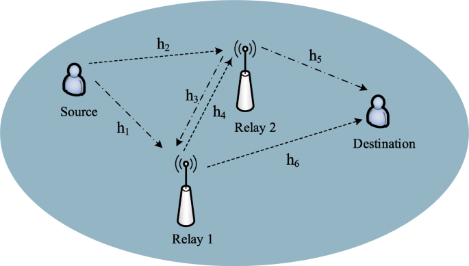
A sample NOMA-based two-path successive AF relay system
As a>0 and b>0 hold, it can be concluded that \((b + \sqrt {b(b - a p_{max})})/a > b/a = (f_{1} f_{5} p_{max} + f_{3} f_{5} p_{r} + f_{5})/(f_{1} f_{5} - f_{5} f_{6} - f_{3} f_{6} - f_{3} f_{5}) > p_{max}\), which conflicts with the pr+ps=pmax constraint, and so it should be excluded. Moreover, it can also be concluded that \(0< (b-\sqrt {b(b - {ap}_{max})})/a = b p_{max}/(b + \sqrt {b(b -a p_{max})}) < (b p_{max})/b = p_{max}\), which is practical under the given constraint. Hence, the feasible scenario is \(p_{max}^{r} < (b - \sqrt {b(b -{ap}_{max})})/a\) when a>0.
The solution of (16) can be expressed as \(p_{r} = [b \pm \sqrt {b(b - a p_{max})}]/a\). As b−apmax>0 always holds, when a>0, the solution \(p_{r} = [b - \sqrt {b(b-ap_{max})}]/a < p_{max}\) is feasible. On the other hand, when a<0, the solution \(p_{r} = [b - \sqrt {b(b-ap_{max})}]/a < p_{max}\) is feasible. Consequently, the available solution is (18) no matter for a>0 or a<0.

Abbreviations
- 5G:
-
Fifth generation
- AF:
-
Amplify-and-forward
- DF:
-
Decode-and-forward
- FIC:
-
Full interference cancellation
- KKT:
-
Karush-Kuhn-Tucher
- NOMA:
-
Non-orthogonal multiple access
- OFDM:
-
Orthogonal frequency division multiplexing
- QoS:
-
Quality-of-service
References
Y. Sun, D. W. K. Ng, Z. Ding, R. Schober, Optimal Joint Power and Subcarrier Allocation for Full-Duplex Multicarrier Non-Orthogonal Multiple Access Systems. IEEE Trans. Commun.65(3), 1077–1091 (2017).
S. M. R. Islam, N. Avazov, O. A. Dobre, K. Kwak, Power-domain non-orthognal multiple access (NOMA) in 5G systems: potentials and challenge. IEEE Commun. Surveys Tuts.19(2), 721–742 (2017).
Z. Ding, Y. Liu, J. Choi, Q. Sun, M. Elkashlan, C. -L. I. H. V. Poor, Application of non-orthogonal multiple access in LTE and 5G networks. IEEE Commun. Mag.55(2), 185–191 (2017).
Z. Ding, X. Lei, G. K. Karagiannidis, R. Schober, J. Yuan, V. K. Bhargava, A survey on non-orthogonal multiple access for 5G networks: research challenges and future trends. IEEE J. Sel. Areas Commun.35(10) (2181).
Z. Hasan, H. Boostanimehr, V. K. Bhargava, Green cellular networks: a survey, some research issues and challenge. IEEE Commun. Survey Tuts.13(4), 524–540 (2011).
S. Wang, R. Ruby, V. C. M. Leung, Z. Yao, X. Liu, Z. Li, Sump-Power Minimization Problem in Multisource Single-AF-Relay Networks: A New Revisit to Study the Optimality. IEEE Trans. Veh. Technol.66(11), 9958–9971 (2017).
J. -B. Kim, I. -H. Lee, Non-orthogonal multiple access in coordinated direct and relay transmission. IEEE Commun. Lett.19(11), 2037–2040 (2015).
J. -B. Kim, I. -H. Lee, Capacity analysis of cooperative relaying systems using non-orthogonal multiple access. IEEE Commun. Lett.19(11), 1949–1952 (2015).
Q. Zhang, Z. Liang, Q. Li, J. Qin, Buffer-aided non-orthogonal multiple access relaying systems in Rayleigh fading channels. IEEE Trans. Commun.65(1), 95–106 (2017).
S. Luo, K. C. Teh, Adaptive transmission for cooperative NOMA system with buffer-aided relaying. IEEE Commun. Lett.21(4), 937–940 (2017).
A. Mohamad, R. Visoz, A. O. Berthet, in Proc. IEE ICC. Code design for multiple-access multiple-relay wireless channels with non-orthogonal transmission (London, 2015), pp. 2318–2324.
R. Jiao, L. Dai, J. Zhang, R. Machenzie, M. Hao, On the performance of NOMA-based cooperative relaying systems over Rician fading channels. IEEE Trans. Veh. Technol.66(12), 11409–11413 (2017).
Z. Ding, H. Dai, H. V. Poor, Relay selection for cooperative NOMA. IEEE Wireless Commun. Lett.5(4), 416–419 (2016).
M. Xu, F. Ji, M. Wen, W. Duan, Novel receiver design for the cooperative relaying system with non-orthogonal multiple access. IEEE Commun. Lett.20(8), 1679–1682 (2016).
M. F. Kader, S. Y. Shin, Cooperative relaying using space-time block coded non-orthogonal multiple access. IEEE Trans. Veh. Technol.66(7), 5894–5903 (2017).
M. F. Kader, M. B. Shahab, S. Y. Shin, Exploiting non-orthogonal multiple access in cooperative relay sharing. IEEE Commun. Lett.21(5), 1159–1162 (2017).
R. -H. Gau, H. -T. Chiu, C. -H. Liao, C. -L. Wu, Optimal power control for NOMA wireless Networks with relays. IEEE Wireless Commun. Lett.7(1), 22–25 (2018).
J. Men, J. Ge, Non-orthogonal multiple access for multiple-antenna relaying networks. IEEE Commun. Lett.19(10), 1686–1689 (2015).
J. Men, J. Ge, C. Zhang, Performance analysis of nonorthogonal multiple access for relaying networks over Nakagami-m Fading channels. IEEE Trans. Veh. Technol.66(2), 1200–1208 (2017).
S. Zhang, B. Di, L. Song, Y. Li, sub-channel and power allocation for non-orthogonal multiple access relay networks with amplify-and-forward protocal. IEEE Trans. Wirelss Commun.16(4), 2249–2261 (2017).
C. Xue, Q. Zhang, Q. Li, J. qin, Joint power allocation and relay beamforming in nonothogonal multiple access amplify-and-foward relay networks. IEEE Trans. Veh. Technol.66(8), 7558–7562 (2017).
X. Liang, Y. Wu, D. W. K. Ng, Y. Zuo, S. Jin, H. Zhu, Outage performance for cooperative NOMA transmission with an AF relay. IEEE Commun. Lett.21(3), 664–667 (2017).
D. Deng, L. Fan, X. Fei, W. Tan, D. Xie, Joint user and relay selection for cooperative NOMA networks. IEEE Access.5:, 20220–20227 (2017).
W. Shin, H. Yang, M. Vaezi, J. Lee, H. V. Poor, Relay-aided NOMA in uplink cellular networks. IEEE Sig. Proc. Lett.24(12), 1842–1846 (2017).
Z. Yang, Z. Ding, Y. Wu, P. Fan, Novel relay selection strategies for cooperative NOMA. IEEE Trans. Veh. Tehnol.66(11), 10114–10123 (2017).
Y. Liu, G. Pan, H. Zhang, M. Song, Hybrid decode-forward & amplify-forward relaying with non-orthogonal multiple access. IEEE Access.4:, 4912–4921 (2016).
C. Zhong, Z. Zhang, Non-orthogonal multiple access with cooperative full-duplex relaying. IEEE Commun. Lett.20(12), 2478–2481 (2016).
B. Zheng, X. Wang, M. Wen, F. Chen, NOMA-based multi-pair two-way relay networks with rate spliting and group decoding. IEEE J. Sel. Areas Commun.34(10), 2328–2341 (2017).
Z. Wei, D. W. K. Ng, J. Yuan, H. Wang, Optimal Resource Allocation for Power-Efficient MC-NOMA With Imperfect Channel State Information. IEEE Trans. Commun.65(9), 3944–3961 (2017).
S. Wang, H. Ji, Distributed power allocation scheme for multi-relay shared-bandwidth (MRSB) wireless cooperative communication. IEEE Commun. Lett.16(8), 1263–1265 (2012).
Acknowledgements
Not applicable.
Funding
This work was supported by the Open Project Program of the Key Laboratory of Universal Wireless Communications (2016-KFKT-2016104), Ministry of Education, the Beijing University of Posts and Telecommunications, the National natural Science Foundation of China (61771414) and the Natural Science Foundation of Hunan Province of China (2017JJ2249).
Availability of data and materials
Not applicable.
Author information
Authors and Affiliations
Contributions
SW was responsible for the mathematical derivation and paper writing. SC was responsible for the numerical simulation. RR was responsible for the derivation checking and language smoothing. All authors read and approved the final manuscript.
Corresponding author
Ethics declarations
Competing interests
The authors declare that they have no competing interests.
Publisher’s Note
Springer Nature remains neutral with regard to jurisdictional claims in published maps and institutional affiliations.
Additional information
Authors’ information
Shiguo wang received the Master and Ph D. degrees in power electronics and power transmission from Xiangtan University and in information communication systems from the Beijing University of Posts and Telecommunications, China, in 2004 and 2010, respectively. He is currently a professor in the key Laboratory of Intelligent Computing and Information Processing, Ministry of Education, Xiangtan University, Xiangtan, 411105, China. From March 2015 to March 2016, he was a visiting scholar in the University of British Columbia (UBC), and cooperated with Prof. Victor C. M. Leung. He has co-authored more than 20 technical papers in international journals and conference proceedings. His research interests are in wireless cooperative communication, cognitive networks, and small-cell backhaul networks.
Rukhsana Ruby obtained her Masters and PhD degrees from University of Victoria and the University of British Columbia on 2009 and 2015, respectively. Her resource interest includes resource management and optimization in wireless networks. She published more than 20 papers in top-level journals and conferences. She now is a post doctor in Shenzhen University.
Shu Cao is a master in Xiangtan University.
Rights and permissions
Open Access This article is distributed under the terms of the Creative Commons Attribution 4.0 International License (http://creativecommons.org/licenses/by/4.0/), which permits unrestricted use, distribution, and reproduction in any medium, provided you give appropriate credit to the original author(s) and the source, provide a link to the Creative Commons license, and indicate if changes were made.
About this article

Cite this article
Wang, S., Cao, S. & Ruby, R. Optimal power allocation in NOMA-based two-path successive AF relay systems. J Wireless Com Network 2018, 273 (2018). https://doi.org/10.1186/s13638-018-1286-z
Received:
Accepted:
Published:
DOI: https://doi.org/10.1186/s13638-018-1286-z