
Abstract
Self-organizing networks (SONs) are expected to minimize operational and capital expenditure of the operators while improving the end users’ quality of experience. To achieve these goals, the SON solutions are expected to learn from the environment and to be able to dynamically adapt to it. In this work, we propose a learning-based approach for self-optimization in SON deployments. In the proposed approach, the learning capability has the central role to perform the estimation of key performance indicators (KPIs) which are then exploited for the selection of the optimal network configuration. We apply this approach to the use case of dynamic frequency and bandwidth assignments (DFBA) in long-term evolution (LTE) residential small cell network deployments. For the implementation of the learning capability and the estimation of KPIs, we select and investigate various machine learning and statistical regression techniques. We provide a comprehensive analysis and comparison of these techniques evaluating the different factors that can influence the accuracy of the KPI predictions and consequently the performance of the network. Finally, we evaluate the performance of learning-based DFBA solution and compare it with the legacy approach and against an optimal exhaustive search for best configuration. The results show that the learning-based DFBA achieves on average a performance improvement of 33 % over approaches that are based on analytical models, reaching 95 % of the optimal network performance while leveraging just a small number of network measurements.
1 Introduction
In recent years, the fourth generation (4G) mobile networks have been rapidly growing in size and complexity. Operators are continuously seeking to improve the network capacity and the QoS by adding more cells of different types to the current deployments consisting of macro-, micro-, pico-, and femtocells. These heterogeneous deployments are loosely coupled, increasing the complexity of 4G cellular networks. This increase in complexity brings a significant growth in the operational and the capital expenditures (OPEX/CAPEX) of the mobile network providers. To reduce these costs on a long-term scale, operators are seeking network solutions that will provide automatic network configuration, management, and optimization and that will minimize the necessity for human interventions. In 2008, the next-generation mobile networks (NGMN) alliance recommended self-organizing networks (SONs) as a key concept for next-generation wireless networks and defined operator use cases in [1]. Shortly after, the SON concept was recognized by the Third-Generation Partnership Project (3GPP) as an essential functionality to be included in the long-term evolution (LTE) technology and consequently it was introduced into the LTE standard in [2]. SONs are expected to reduce the OPEX/CAPEX and to increase the capacity and the QoS in future cellular networks. All self-organizing tasks in SONs are described at a high-level by the following features: self-configuration, self-healing, and self-optimization.
Recent studies show that roughly 80 % of mobile data traffic is indoor [3]. Still, operators are failing at providing good QoS (coverage, throughput) to the indoor users. In order to solve these issues while saving OPEX/CAPEX, operators are deploying small cells. These are low cost cells that can be densely deployed in residential areas and which are connected to the core network via broadband. In current early LTE small cell deployments, various technical issues have been detected. Small cells are increasingly being deployed according to traffic demands rather than by traditional cell planning for coverage. Such LTE small cell networks are characterized by unpredictable interference patterns, which are caused by the random and dense small cells placements, the specific physical characteristics of the buildings (walls, building material, etc.), and the distance to outdoor cells, e.g., macro or micro base stations. Thus, such deployment scenarios are characterized by complex dynamics that are hard to model analytically. However, in the research literature, solutions are often proposed based on simplified models, e.g., assuming interference models with uniform distribution of small cells over the macrocell coverage, which differs significantly from realistic urban deployments [4]. Therefore, in these kinds of deployments, the classical network planning and design tools become unusable, and there is an increasing demand for small cells solutions that are able to self-configure and self-optimize [5].
Recently, the authors of [6] suggested that the cognitive radio network (CRN) paradigm could be used in SONs to increase their overall level of automation and flexibility. CRNs are usually seen as predecessors of SONs. The CRN paradigm was initially introduced in 1999 by Mitola and Maguire [7] in the context of a cognitive radio, and since then, it evolved significantly and received a lot of attention by the scientific community. The cognitive paradigm can be implemented in the network by adding an autonomous cognitive process that can perceive the current network conditions, and then plan, decide, and act on those conditions [8]; and while doing so, it is learning and adapting to the environment. This cognitive approach could be applied to SONs as an autonomous process for self-optimization and self-healing, which can perform a continuous optimization of the network parameters and their adaptation to the changes in the environmental conditions. Additionally, because of its learning capabilities, a cognitive approach can be used to meet a plug-and-play requirement for SONs according to which the device should be able to self-configure without any a priori knowledge about the radio environment into which the radio device will be deployed. Many different network optimization problems are successfully addressed by using a CRN approach based on machine learning (ML) [9].
Several network infrastructure providers have also been developing SON solutions based on machine learning and big data analytics. For example, Reverb, one of the pioneers in self-optimizing network software solutions, has created a product called InteliSON [10], which is based on machine learning techniques and its application to live networks results in lower drops, higher data rates, and lower costs for operator. Similarly, Zhilabs and Stoke [11] are developing solutions based on big data analytics. Samsung developed a product called Smart LTE [12] that is leveraging on SON solution that gathers radio performance data from each cell and adjusts a wide array of parameters at each small cell directly.
Similarly to the previously described industrial approaches, in this work, we focus on the application of ML to improve SON functionalities by providing a more accurate estimates of the key performance indicators (KPIs) as a function of the network configuration. The KPIs are mainly important for operators to detect changes in the provided quality of service (QoS) and QoE, for example, in order to reconfigure the network in response to a detected degradation in QoS. The estimation of the KPIs based on a limited network measurements is one of the main requirements of the minimization of drive tests (MDT) functionality and represents a key element for the realization of the big data empowered SON approach introduced in [13]. In this work, we apply learning-based LTE KPI estimation approach to the specific use case of LTE small cell frequency and bandwidth assignment. We investigate the potential of LTE’s frequency assignment flexibility [14] in small cell deployments, i.e., exploiting the possibility of assigning different combinations of carrier frequency and system bandwidth to each small cell in the network in order to achieve performance improvements. Currently, most LTE small cell deployments rely on same-frequency operation with the reuse factor of one, whose main objective is to maximize the spectral efficiency. However, the spectrum reuse factor is subject to a trade-off between spectral efficiency and interference mitigation. Since interference may become a critical issue in unplanned dense small cell deployments, reconsidering spectrum reuse factors in this kind of deployments may be necessary. Moreover, the same-frequency operation is not expected to be the standard practice in the future, since additional spectrum will be available at higher frequencies, e.g., 3.5 GHz [15]. Thus, for the future network deployments, it will be more relevant to consider band-separated local area access operating on higher-frequency bands, with the overlaid macro layer operating on lower cellular bands.
In this work, we investigate how to exploit this flexibility in order to maximize the performance of small cell network deployments. We show that the proposed learning-based approach for KPI estimation can be successfully employed to effectively optimize such multi-frequency multi-bandwidth small cells deployment strategy.
2 Related work and proposed contribution
Frequency assignment is one of the key problems for the efficient deployment, operation, and management of wireless networks. For earlier technologies, such as 2G and 3G networks as well as Wi-Fi access point deployments, relatively simple approaches based on generalized graph coloring [16] were sufficient to obtain a good performance. This is because the frequency assignment for these networks was often orthogonal and with a low degree of frequency reuse, and the runtime scheduling of radio resources had a highly predictable behavior due to the simplicity of the methods used. Additionally, due to the predictable system load, the frequency assignment was often based on static planning, which could be done easily offline.
However, the new 4G technologies, such as LTE, adopt a more flexible spectrum access approach based on dynamic frequency assignment (DFA) and inter-cell interference coordination in order to allow a high-frequency reuse and capacity. In particular, DFA is recognized as one of key aspects for high performance small cell deployments [17]. According to DFA, the available spectrum is allocated to base stations dynamically as a function of the channel conditions to meet given performance goals. Furthermore, the LTE technology is highly complex due to the inclusion of advanced features such as OFDMA and SC-FDMA, adaptive modulation and coding (AMC), dynamic MAC scheduling, and hybrid automatic repeat request (HARQ) [14]; hence, it is much more difficult to predict the actual system capacity in a given scenario than it was for previous mobile technologies. Because of this, it is very challenging to design a DFA solution that can work well not only on paper but also in a realistic LTE small cell deployment. On this matter, while several publications recently appeared in the literature deal with the general problem of LTE resource management, considering aspects ranging from power control [18] to frequency reuse between macro and small cells [19], only few works focus on DFA for small cell networks. Among these, we highlight [20] and [21] whose authors propose DFA solutions based on graph coloring algorithms. The key aspect of these papers, and of many other similar works, is that they assume that the rate achieved on a specific channel is given by simple variants of Shannon’s capacity formula, thus neglecting some important aspects that affect the performance of an LTE system, such as MAC scheduling, HARQ, and L3/L4 issues. Doing this yields significant errors in the estimation of the actual system capacity, possibly resulting in sub-optimal or even badly performing frequency assignments even in relatively small networks. Because of this, we argue that solutions like [20] and [21] are not suitable for real deployments.
Additionally, as argued in [22], the existing techniques for femtocell-aware spectrum allocation need further investigation, i.e., co-tier interference and global fairness are still open issues. The main issue is to strike a good balance between spectrum efficiency and interference, i.e., to mitigate the trade-off between orthogonal spectrum allocation and co-channel spectrum allocation. Still, the existing approaches are highly complex, difficult to be implemented by the operator, and they mainly aim to address the cross-tier spectrum-sharing issues.
We believe that a learning-based approach can address successfully these issues while keeping the overall implementation and computational complexity very low. The main advantage of machine learning approach over other techniques is its ability to learn the wireless environment and to adapt to it. To the best of our knowledge and according to some of more recent surveys, i.e., [22], there is only little work in the literature that is considering a machine learning for frequency assignment in small cell networks. In [23], the authors propose a machine learning approach based on reinforcement learning in a multi-agent system according to which the frequency assignment actions are taken in a decentralized fashion without having a complete knowledge on actions taken by other small cells. Such decentralized approach may lead to frequent changes in frequency assignments, which may cause unpredictable levels of interference among small cells and degradation of performance.
In this work, we apply different machine learning and advanced regression techniques in order to predict the performance that a user would experience in an LTE small cell network by leveraging a small sample of performance measurements. These techniques take as inputs different frequency configurations and measured pathloss data and hence allow to estimate the impact of configuration changes on various KPIs. Differently to the previously described work, in our approach, frequency assignments of the small cells are determined in a centralized fashion, by selecting the parameters which will lead to the best network performance.
Summarizing, the key contributions of this paper are the following:
-
1.
We propose a learning-based approach for LTE KPI estimation, and we study its application to the use case of dynamic frequency and bandwidth assignment (DFBA) for self-organizing LTE small cell networks.
-
2.
We select and investigate various ML and statistical regression techniques for predicting network and user level KPIs accounting for the impact on the performance of the whole LTE stack, based on small number of measurements. Our focus is specifically on well-established machine learning and regression techniques rather than on developing our own ad hoc solutions. Furthermore, to the best of our knowledge, this study is the first one to include both ML and regression techniques in a comparative integrated study applied to LTE SONs.
-
3.
We study the impact of the choice of covariates (measurement or configuration information made available to the performance prediction algorithm) and different sampling strategies (effectively deciding which measurements of network performance to carry out in a given deployment) on the efficiency of the KPI prediction. Additionally, the prediction performance is tested for different network configurations, different sizes of training sets, and different KPIs.
-
4.
We evaluate the performance of a DFBA solution based on the proposed learning-based KPI estimation, comparing with legacy approach as well as with an optimal exhaustive search approach.
3 Learning-based dynamic frequency and bandwidth assignment
3.1 LTE system model
We first summarize the aspects of the LTE technology that are relevant for our study. We consider the downlink of an LTE FDD small cell system. The LTE downlink is based on the orthogonal frequency division multiple access technology (OFDMA). The OFDMA technology provides a flexible multiple-access scheme that allows the transmission resources of variable bandwidth to be allocated to different users in the frequency domain and different system bandwidths to be utilized without changing the fundamental system parameters or equipment design [14]. In LTE, as far as frequency assignment and radio resource management are concerned, a small cell is an ordinary base station (eNodeB); the main differences with respect to a macro/micro eNodeB are its location (typically indoor), and its smaller transmission power. As in this work we focus on small cell deployments in the remainder of this paper, we will use the term eNodeB and small cells interchangeably.
According to the LTE physical layer specifications [24], radio resources in the frequency domain are grouped in units of 12 subcarriers called resource blocks (RBs); the subcarrier spacing is 15 kHz, thus one RB occupies 180 kHz. In this work, we consider the following network parameters for the LTE downlink: (1) the system bandwidth B and (2) the carrier frequency f c . Each LTE eNodeB operates using a set of B contiguous RBs; the allowed values for B are 6, 15, 25, 50, 75, and 100 RBs, which correspond to a system bandwidth of 1.4, 3, 5, 10, 15, and 20 MHz, respectively [24]. These RBs are centered around the carrier frequency f c , which is constrained to be a multiple of 100 kHz since the LTE channel raster is 100 kHz for all bands [25]. The setting of B and f c can be different for each eNodeB, which gives significant degrees of freedom for the selection of the frequency assignment. We highlight that in a scenario with small cells that have the same value of B, but different value of f c , there will be some RBs that are fully overlapped, some that are orthogonal, and some that are partially overlapped, as shown in the example of Fig. 1.

The partial frequency overlapping between two femtocells which have different f c , but the same B=6R B; f oi is the lower bound of frequencies being used by the i-th small cell, and f bi is the upper bound
3.2 Optimization problem and real system constraints
Taking into account the system model described in Section 3.1, our specific optimization problem consists of selecting, for each deployed eNodeB i=1,…,N, the frequency \({f_{c}^{i}}\) and the system bandwidth B i that achieves the best network performance in terms of selected KPI. The number of possible configurations, C, is exponential with N; the base of the exponent depends of the number of allowed combinations of f c and B for each eNodeB, which depends on the total bandwidth available for the deployment by the operator and is constrained by the operator’s deployment policy. Let \(x_{\text {conf}}^{(i,j)}=\left (f_{c}^{(i,j)},B^{(i,j)}\right)\) be the configuration of the i-th eNodeB in the configuration j; then, the j-th network configuration may be represented as a vector \(\vec {x}^{j}=\left [x_{\text {conf}}^{(1,j)},\dots,x_{\text {conf}}^{(N,j)}\right ]\), where j=1,…,C. Let \(\gamma _{kpi}^{j}\) be the network performance for the selected KPI. The network configuration that maximizes the network performance is formally given by
If the values \(\gamma _{kpi}^{j}\) are known for all frequency and bandwidth configurations, then the \(\vec {x^{\mathrm {(opt)}}}\) can be found by performing an exhaustive search on the set of samples \(\left (\vec {x}^{j},\gamma _{kpi}^{j}\right)\). However, the application of exhaustive search is not feasible in a real system. The practical constraints of this solution are the cost and the time of performing the network measurements for all possible configurations. The measurements may be obtained by performing drive tests, but as these tests are expensive for the operator, the number of tests would need to be very limited. To reduce costs, the MDTs measurements may be used. Even so, time would be a significant constraint, since the time to obtain all measurements linearly grows with the number of possible configurations.
As an example, in a four small cell network deployment with a total available bandwidth of 5 MHz, considering f c values multiple of 300 kHz (three times the LTE channel raster, i.e., one third of the possible frequencies), and limiting the choice of B to \(\mathcal {B} = \{6, 15, 25\}\) for simplicity, there are already 4625 physically distinct configurations. For a five small cell network, this number grows to 34,340. If the measurement time per configuration is only 1 h, then the time necessary to gather measurements for a four small cell network is 193 days and for a five small cell network is close to 4 years. In order to overcome this constraint, we aim at designing a solution that is capable of performing nearly optimal while leveraging only a limited number of KPI measurements.
Finally, we consider another two constraints of the real small cell deployments: the number of possible configurations, C, and the frequency of the configuration changes in the network. Even if an LTE carrier could be positioned anywhere within the spectrum respecting the channel raster constraint, and the basic LTE physical-layer specification does not say anything about the exact frequency location of an LTE carrier, including the frequency band, the number of allowed combinations needs to be limited for practical reasons [15], e.g., to reduce search time when an LTE terminal is activated. As we will show in this work, even with a limited number of combinations of parameters, significant performance gains can be achieved.
Obviously, these parameters cannot be changed frequently, so one could question time-scale applicability of this solution to real small cell deployments. This question was raised in more general context for SONs, and in one recent study, the authors of [26] argue that SONs based on longer time scale system dynamics (e.g., user concentration changes, user mobility patterns, etc.) can lead to better performance than solutions that are based on dynamics of shorter time scales (e.g., noise, fast fading, users mobility).
3.3 Proposed approach
In a nutshell, our goal is to design a general framework for LTE network performance prediction and optimization, that is easy to deploy in a real LTE system and able to adapt to the actual network conditions during normal operation. In Fig. 2, we illustrate our proposed approach. As shown in the figure, we focus mainly on LTE indoor small cell network deployments and, in terms of evaluation, on the typical LTE residential dual-stripe scenario described in [27]. This scenario characterizes not only interactions among neighboring small cells within the same building but also among small cells belonging to adjacent buildings. According to our approach, the measurements are gathered from both LTE users and LTE small cells. On the user side, we gather measurements related to the performance achieved by user, i.e., throughput, and delay, and the corresponding measurements related to channel conditions, i.e., SINR per RB. On the small cells side, we gather radio link control (RLC) and MAC layer statistics, and various throughput performance measurements. These measurements are then used to calculate different metrics which are then used for network performance predictions by the LTE KPI Prediction Engine. This engine is leveraging different machine learning and regression methods to realize the LTE KPI prediction functionality. The predicted LTE KPI values are then forwarded to the DFBA Optimization Engine which is using these values together with network measurements to inspect how near the current network performance is to the estimated optimal performance for the currently measured network conditions. If the DFBA Optimization Engine estimates that the change in network configuration will compensate possible trade-offs (e.g., interruption in service), it schedules the reconfiguration of the frequency and bandwidth assignment.

Proposed learning-based approach
Our approach follows the centralized SON (CSON) architecture, according to which there is a centralized node that oversees operation of all small cells and controls their behavior. In CSON architecture, the centralized node receives inputs from small cells and determines their configuration. Thus, the LTE KPI Prediction Engine and the DFBA Optimization Engine are placed at the centralized node. Since the configuration parameters are not going to be changed frequently, the proposed solution should not be affected by the latency due to the communication exchange between small cells and the centralized node. Also, the network overhead is low, since the measurement information from the small cells to the central node can be scheduled per best-effort basis. Note that this architecture is compliant with the control plane solution for MDT which is discussed in 3GPP TR32.827 [28]. Thus, the main message exchanges in our approach are between user equipments (UEs) and small cells and between small cells and the centralized management node, and all the interfaces needed for implementing our solution are already present in the standard.
The main contribution of the proposed approach is the learning-based LTE KPI performance estimation. Even if in this work we apply this approach to the frequency and bandwidth assignment use case, we argue that this approach is much more general and may be used for a larger set of configuration parameters and for different utility-based network planning and optimization tasks [9], where the accurate prediction of KPIs are necessary for an effective optimization.
3.4 LTE KPI prediction engine
To realize the LTE KPI prediction engine, we propose a learning-based approach according to which different KPIs are accurately predicted by using regression analysis and machine learning techniques based on basic pathloss and configuration information combined with a limited number of feedback measurements that provide the throughput and the delay metrics for a particular frequency and bandwidth setting. As discussed in Section 3.2, we aim at designing a solution that requires a minimal amount of training for active exploration. Moreover, the prediction engine should be able to predict different KPIs, e.g., the network-wide and per-user LTE KPIs. To achieve all these requirements and to select the best candidate for the prediction engine, we study and compare the performance of various classical and modern prediction techniques. We list and explain these techniques in Section 3.5.
These prediction techniques leverage various parameters, metrics, and derived inputs. The latter are usually called covariates or regressors in the statistical and machine learning literature. Among the covariates being used in this paper, the most are being calculated by using the SINR/MAC throughput mapping. This mapping represents the network MAC layer throughput calculation based on the actual network measurements. We calculate this mapping in the following way. According to the LTE standard, UEs are periodically reporting to the base station a channel quality indicator (CQI) per each subband and wideband. We use this value at the MAC layer of the base station for AMC mapping, i.e., to determine the size of the transport block (TB) to be transmitted to the UE. A typical AMC behavior is to select a TB size that yields a BLER between 0 and 10 % [29]; the TB size for each given modulation and coding scheme and number of RBs are given by the LTE specification in [30].
Moreover, we investigate the performance for different combinations of covariates. Since the covariates can be combined on a per-RB basis or aggregated together in various ways (such as considering the minimum or the sum of SINRs over the band), the number of different combinations of covariates is very large. Here, we limit our attention to a small number of representative combinations summarized in Table 1.
Additionally, we consider the effect on prediction performance of different sampling methods, i.e., random and stratified sampling. In statistics, stratified sampling is obtained by taking samples from each stratum or sub-group of a population, i.e., a mini-reproduction of the population is achieved; conversely, according the random sampling method, each sample is chosen entirely by chance in order to reduce the likelihood of bias. While stratified sampling requires more effort for data preparation, it is appealing for its higher prediction accuracy in scenarios where the performance varies among different sub-groups of population or sampling regions. For the stratified sampling method, we define the sampling regions by calculating the aggregated network throughput based on the SINR/MAC throughput mapping previously described.
Finally, we analyze performance prediction by means of goodness of fit metrics, such as the prediction error in network-wide and per-user throughput estimation, evaluating how they depend on the size of the training set. This allows us to determine the ability of the proposed solution to learn during real-world operation.
3.5 Statistical and machine learning methods for LTE KPI prediction engine
In this section, we provide an overview of the different statistical and machine learning methods being studied for the realization of the LTE KPI prediction engine. We begin with a basic overview of the principles and terminology involved, and then give a concise summary on the principles of the methods used. For further information on the prediction techniques being used, the interested reader is referred to [31] and [32].
The objective of all of the methods considered, regardless of whether statistical or machine learning based, is to find a function that predicts the value of a dependent variable y=f(x 1,…,x n ) as a function of various predictors or covariates x i . Usually, this is done by conducting a limited number of experiments that yield the value of y for known values of the covariates that are then used to fit or train the model. The functional form of the model as well as the training procedure used are the main differences between the different methods. In our case, the y corresponds to a performance metric of interest, and the different x i are measurements of network conditions (signal-to-interference-plus-noise ratio (SINR) values for different nodes) as well as available prior data (such as theoretical MAC layer throughput at given SINR).
The simplest method used for establishing a baseline prediction performance is LM that simply models y as a linear function of the covariates, as in
The coefficients a i are determined based on the training data for example by minimizing the root mean squared error (RMSE) of the predictor. Linear regression also has in our context a simple communication-theoretic interpretation: in the high SINR regime, linear functions approximate well the Shannon capacity formula, and y becomes simply the best approximation of the network throughput as a optimal weighted sum of the individual Shannon capacity estimates. Thus, linear regression can be used as an improved proxy for simple Shannonian SINR-based network capacity models. Simple generalization of this basic scheme is to apply a transformation function to each of the terms a i x i . The generalized regression techniques thus obtained are usually called projection pursuit regression (PPR) methods.
The simplest non-traditional prediction method we consider is the K nearest neighbors algorithm (KNN for short). For KNN, we consider the covariates x i as defining a point in an Euclidean space, with the value of the y obtained from the corresponding experiment being assigned to that point. When predicting y for \(x^{\prime }_{i}\) for which experimental data is not available, we find the K nearest neighbors of the point \(x^{\prime }_{i}\) from the training data set in terms of the Euclidean distance. Our prediction is then the distance-weighted average of the corresponding values of y. The KNN algorithm is an example of a non-parametric method that requires no estimation procedure. This makes it easy to apply, but limits both its ability to generalize beyond the training data and the amount of smoothing it can perform to counter the effects of noise and other sources of randomness on the predictions.
A much more general and powerful family of regression techniques is obtained by considering trees of individual regression models. The model corresponds to a tree graph, with each non-leaf vertex corresponding to choosing a subspace by imposing an inequality of some of the x i . The leaves of the tree finally yield the predictions y as the function of the ancestor vertices partitioning the space of x i into subsequently finer subspaces. The various regression tree algorithms proposed in the literature differ mainly in the method used to choose the partitioning in terms of the covariates x i , as well as in the way training data is used to find the optimum selection of decision variables in terms of the chosen partitioning scheme. We consider both boosting (boosted tree (BTR)) and bagging (TBAG) in the process of finding optimal regression tree. Of these, bagging uses bootstrap (sampling with replacement to obtain large number of training data sets from a single one) with different sample sizes to improve the accuracy of the parameter estimates involved. Boosting on the other hand performs retraining of the model several times, with each iteration giving an increased weight to samples for which the previous iterations yielded poor performance result. The final prediction from a boosted tree is a weighted average of the predictions from the individual iterations. In general, regression trees are a very powerful and general family of prediction methods that should be considered as a potential solution to any non-trivial prediction or learning problem.
Support vector machines (SVMs) are a type of the machines not only often used for classification and pattern recognition but can also be used for regression problems. These methods have efficient training algorithms and can represent complex nonlinear functions. The core of this method is the transformation of the studied data into a new, often higher dimensional, space so that this data is linearly separable in this new space, and thus, the classification or regression is possible. The representation of data using a high-dimensional space carries the risk of overfitting. SVMs avoid this by finding the optimal linear separator, a hyper-plane that is characterized by the largest margins between itself and the data samples from both sides of the separator. A separator is obtained by the solution of a quadratic programming optimization problem, which is characterized by having a global maximum, and is formulated using dot products between the training data and the support vectors defining the hyperplanes. While it is rare that a linear separator can be found in the original input space defined by the x i , this is often possible in the high-dimensional feature space obtained by mapping the covariates with the kernel function. In the following, we use SVMs with basic radial basis functions for regression.
The last family of machine learning techniques we consider in our study is that of self-organizing maps also known as Kohonen networks (KOH). These form a family of artificial neural networks, for which each neuron (a vertex on a lattice graph) carries a vector of covariates initialized to random values. The training phase iterates over the training data set, finds the nearest neighbor to each vector of covariates from this set and the neural network, and updates the corresponding neuron and its neighbors to have higher degree of similarity with the training vector. Over time, different areas of the neural network converge to correspond to different common types occurring often in the training data set. While originally developed for classification problems, the Kohonen network can be used for regression by assigning a prediction function (such as the simple linear regression) to each class discovered by the neural network.
The considered KPIs, prediction methods and metrics, regressors, and sampling methods are summarized in Table 2. We use the R environment, and in particular the caret package, as the basis of our computations [32].
4 Performance evaluation
4.1 Evaluation setup
We consider a typical LTE urban dual stripe building scenario defined in [27] and the corresponding simulation assumptions and parameters defined in [33]. In Fig. 3, we show a radio environmental map of one instance of the simulated scenario. Each building has one floor which has eight apartments. The small cells (home eNodeBs) and users are randomly distributed in the buildings. Each home eNodeB has an equal number of associated UEs and is placed in a separate apartment along with its associated UEs. By using the random distribution, we aim at simulating the scenario that corresponds to the greatest extent to a realistic residential small cell deployment. The random placement of small cells in each independent simulation along with the random placement of the users adds to the simulation additional degree of randomness, which is consequently increasing the credibility of obtained simulation results. We concentrate on studying the following network configurations:
-
4 home eNodeBs, 12 users, and a total system bandwidth of 2 MHz
Fig. 3 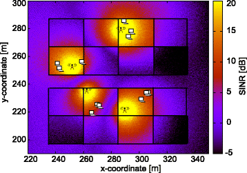
Radio environmental map of dual-stripe scenario with one block of two buildings. Each home eNodeB has connected three UEs that are located in the same apartment
-
4 home eNodeBs, 8 users, and a total system bandwidth of 5 MHz
-
2 home eNodeBs, 20 users, and a total system bandwidth of 2 MHz

For propagation modeling, we use the ITU-R P.1238 model with additional loss factors for internal and external wall penetration. We consider both transmission control protocol (TCP) and user datagram protocol (UDP) as transport layer protocols to investigate the performance of our approach for different types of transport protocol. In both cases, we configure traffic parameters to send packets with a constant rate that can saturate the system. Additionally, we consider the effect of the MAC scheduler on the LTE KPI prediction performance. The purpose of MAC scheduler is to decide which RB will be assigned to which UE; different policies are used for this purpose, resulting in different performance trade offs. We select two schedulers that are widely used as a reference in literature: round robin (RR) and proportional fair (PF). For more information on MAC schedulers, the interested reader is referred to [34]. To avoid the effects of the network initializations and starting up of the user applications, we neglect the first interval of 5 s of each simulation execution. We configure simulations by using different combinations of B and f c , and we configure other network parameters according to Table 3. Different random placements of small cells and users are achieved by running each simulation configuration with different values of the seed of the random number generator.
To simulate the scenarios, we use the ns-3-based LTE-EPC network simulator (LENA) [35] which features an almost complete implementation of the LTE protocol stack, from layer two above, together with an accurate simulation model for the LTE physical layer [29]. The use of such detailed simulator provides a performance evaluation which is reasonably close to that of an experimental LTE platform.
4.2 Results on the correlation between covariates and KPIs
We begin by illustrating the challenges of MAC layer throughput prediction based on a SINR metric. For this analysis, we select the Sum SINR, Sum/THR Mapping, and Min SINR per RB covariates that were introduced in Section 3.4. The Sum SINR covariate is calculated as the raw sum of SINRs per RB. The SUM/THR Mapping represents the MAC layer throughput calculated as a function of the raw sum of SINRs per RB according to the throughput calculation based on the the AMC scheme, which is explained in Section 3.4. The Min SINR per RB covariate is the minimum SINR perceived per RB. The SINR metric is calculated by leveraging on the pathloss measurements gathered at each UE. In Fig. 4, we show the actual measured system-level MAC layer throughput as a function of either Sum SINR or Sum/THR Mapping based on 337 simulation results. Points in the figures correspond to measurements obtained from different simulation executions.

Actual measured performance vs. pathloss-based SINR and 3GPP based mapping of these values to MAC throughput. System bandwidth of 2 MHz, 4 small cells with 3 associated users each
From Fig. 4 a, b we note that (1) a low positive correlation is present between actual measured throughput and covariates, which confirms the need for advanced prediction techniques for KPI predictions, and (2) the correlation between the system-level MAC throughput and the covariates, Sum SINR and Sum/THR Mapping, is very similar for proportional fair and round robin schedulers, i.e., it is expected that the KPI prediction engine that is predicting system-level KPIs by using these covariates will perform equally good regardless which MAC scheduler is being used at eNodeBs. This is not the case for the user-level KPI estimation. Namely, from Fig. 4 c, we note that when the proportional fair scheduler is used there is no linear correlation between the MAC throughput and Sum SINR/THR Mapping, while when the round robin scheduler is used, there is a positive correlation. This indicates that the choice of MAC scheduler significantly affects the correlation function between the actual measured MAC throughput and the selected covariate, when the user-level KPIs are predicted. This can be explained by the fact that the round robin scheduler allocates approximately equal amount of resources to each UE, while the resources allocated by the proportional fair scheduler strongly depend on the actual environment, e.g., distributions of small cells and users, and on the channel conditions of all users; thus, the KPIs obtained when using round robin scheduler should be easier to predict. Still, the results obtained for round robin scheduler show large dispersion of correlation. This behavior may be the consequence of assigning the resources to UEs always in the same order during the simulation; thus, if there is a significant difference between SINRs among RB, this will affect the performance of the user. For example, if some user always gets assigned a RB with low SINR, the performance will be poor, even if the average SINR value over all RBs allows for much better performance. Another reason could be that the transport block size assigned to the user is affected by the presence of RB with very low SINR; because of this, in the following, we consider the correlation of Min SINR per RB and MAC Throughput.
In Fig. 5, we illustrate correlations between the KPI and the selected covariates on a much larger data set which contains 4625 samples. These samples are achieved by configuring a larger system bandwidth, 5 MHz, which allows for much larger number of frequency and bandwidth assignment combinations, as we explained in Section 3.2. As we show in the following discussion, the analysis on a larger data set confirms the trends that were observed for a smaller data sets in Fig. 4. In Fig. 5 a, b, we note the strong correlation between the transport protocol type and the measured MAC layer throughput. When the transport protocol is UDP, there is a strong correlation between the MAC Throughput and the Sum SINR/MAC THR Mapping covariate. On the other hand, when TCP is being used, there is a weak correlation, i.e., it is harder to predict the KPIs. This is an expected behavior because of the complex interplay between the TCP congestion control and the LTE PHY, MAC, and RLC layers. We also note from these two figures that there is no strong correlation between MAC Throughput and Min SINR per RB, so that the dispersion of results for the round robin scheduler shown in Fig. 4 c is not caused by assigning the min SINR per RB to UEs. Figure 5 c shows that the correlation remains strong when eNodeBs are configured to use the round robin scheduler instead of proportional fair and that the Sum SINR and the Sum SINR/MAC THR Mapping covariates can be used almost interchangeably for predictions. We also note that the smaller number of users increases the dispersion in the SINR vs. MAC throughput dependency even further.

Actual measured performance vs. pathloss-based SINR, and 3GPP-based mapping of these values to MAC throughput. System bandwidth of 5 MHz. Setup with four small cells each having associated two users in a and b; two small cells each having associated ten users in c
From these results, we note that the correct selection of covariates is fundamental for the robust and effective prediction engine. Moreover, we expect that designing a solution that can perform good in a variety of network configurations, and that can perform equally good while predicting both system-level and user-level KPIs, is a challenging problem.
4.3 Performance of prediction methods
Following the conclusions derived in Section 4.2, we select the scenario setup and regressors for the performance comparison of the LTE KPI prediction methods. Namely, we select the configuration that appears the most complex for prediction, i.e., the configuration manifested by low or lack of linear correlation between the predicted KPI and covariates, that is the network configuration in which small cells operate with the proportional fair MAC scheduler and UEs traffic goes over TCP. Additionally, based on a study from Section 4.2, we select the aggregate regressors, since they appear to have a higher correlation with KPI than Min SINR per RB. The total of 4625 samples are obtained by running the small cell network scenario that consists of four small cells with two users associated to each of them, while the total system bandwidth is 5 MHz. The training data for each prediction method is obtained by selecting 10 % of samples by random sampling method. The testing data samples are generated based on measurements for each user in the scenario, with a total of 50 independent samplings and regression fittings samples. We consider the following prediction techniques: bagging tree (TBAG), BTR, KOH, SVM radial (SVM), K-nearest neighbor (KNN), PPR, and linear regression method (LM), all of which we explained in detail in Section 3.5. Finally, in Fig. 6, we show the results of the prediction performance of different prediction methods. For boxplots, the three lines of the box denote the median together with the 25th and 75th percentile, while the whiskers extend to the data point at most 1.5 interquartile ranges from the edge of the box.

Comparison of prediction methods over random sampling of 10 %
As expected for the selected network scenario with a complex non-linear nature of the additional information, the simplest prediction method, LM, has the highest RMSE and consequently the poorest prediction performance ratio. The poor performance of the LM method indicates that analytical models based on Shannonian capacity estimates are also expected to perform poorly. Note also that the gain of more advanced methods over LM lower bounds the gain compared to even simpler schemes, such as full frequency reuse or orthogonalized channelization. More advanced prediction techniques based on regression, PPR and KNN, are computationally extremely fast (≪1m s for the tested sample set), which can thus be useful to offer an intermediate solution in situations in which more computationally expensive methods are not feasible. Among advanced machine learning techniques, SVMs and KOH networks perform the poorest, and the latter technique shows additionally a large variability in the performance prediction accuracy. Both tree-based methods (TBAG and BTR) perform consistently better than all previous methods in terms of raw performance and variability of results; finally, the TBAG method achieves the best prediction performance. This superior performance is expected due to the very nature of TBAG and BTR. Use of bootstrap samples results in both of these methods being essentially not an individual machine learning optimizer, but an ensemble learner conducting voting between large number of individual models. Such combinations of models usually outperform individual ones by wide margin at the cost of larger storage and training overhead [31]. Based on the latter discussion, we conclude that TBAG is the most promising method for the prediction engine.
4.3.1 Prediction performance validation for different sizes of the training set
In the following, we evaluate the prediction performance of TBAG as a function of the size of the training set, i.e., in order to assess how fast it can learn when deployed in an actual scenario. We carry out a performance evaluation study using the same small cell network scenario setup that we used for the comparison of the prediction techniques. We compare TBAG with the LM method in order to analyze the advantage of the application of advanced prediction techniques instead of simple prediction techniques for different sizes of the training set. For this performance evaluation, we define the performance ratio metric as the ratio of the network throughput of the frequency and bandwidth allocation chosen by solving the optimization problem with the considered model to the network throughput of the best possible frequency and bandwidth configuration, i.e., the one that would be allocated by an exhaustive search algorithm. The purpose of this metric is to give a measure of how close a given solution is to the optimal frequency and bandwidth assignment. In Fig. 7, we show the results of the prediction performance for different sizes of the training set. The black lines in the figures show the tendencies in the plot, while the boxplots are generated in the same way as for the results shown in Fig. 6. By observing the RMSE from Fig. 7, we note that for more accurate performance more samples need to be taken, though this does not necessarily translate into a better network optimization performance, which is the case for the LM method. Additionally, we conclude that the benefit of advanced prediction techniques over simpler prediction techniques is not only the ability to learn on a very small sample set but is also the ability to improve its performance over time. Both characteristics are crucial for a real network deployment, as we seek a solution that can work good with minimum a priori knowledge, and that is able to improve performance by exploiting real-time network measurements.

Linear and bagging tree methods for different sizes of the training set (random sampling with 5 to 70 %)
4.3.2 Prediction performance validation for different LTE KPIs and network configurations
We continue the TBAG performance analysis by testing the prediction of different KPIs metric under various network configurations. Specifically, whereas before we evaluated TBAG in the context of optimizing system level KPI, we now focus on the performance prediction of TBAG in terms of user-level KPIs. We evaluate the performance obtained with differently configured small cell network setups. The fixed scenario parameters are the system bandwidth is 2 MHz, network has 4 small cells, and a total of 12 users. We run independent batch simulations that have in common the small cell network topology, but differently configured transport protocols used by UEs’ applications (TCP or UDP) and different MAC scheduler (proportional fair or round robin). Out of the four combinations (two different schedulers, two different transport protocol types) that we evaluated, we illustrate the performance of TBAG vs. LM in Fig. 8 for the two most interesting cases: (1) eNodeBs employing the proportional fair scheduler and UEs traffic going over TCP and (2) eNodeBs employing the round robin scheduler and UEs traffic over UDP. Our results confirm that the TBAG method performs well for different scenario setups. Here, the TBAG method outperforms the LM method, especially in the case of TCP and the proportional fair scheduler (Fig. 8 a, b). We note that the results shown in Fig. 6 also hold on a per-user basis, as well as in more complex and dynamic network scenario (TCP and proportional fair scheduler being used). Figure 8 c, d shows a similar collection of results, but for the case of UDP with the round robin scheduler. Here, even the simple LM method performs nearly optimal due to the simplified higher-layer interactions explained in Section 4.2. These figures confirm the previously formulated hypothesis that the network configuration with the simpler setup (UDP and more simple scheduler, such as round robin) results in a higher predictability.

Random sampling with 10 % of 337 permutations being explored with the linear and the bagging tree regression methods and the aggregate regressor. a, b TCP and proportional fair scheduler. c, d UDP and round robin scheduler. a Normalized performance considering per user optimization. b RMSE over user performance regression fitting with actual measured performance ranging from 538 to 1545 kbps. c Normalized performance considering per user optimization. d RMSE over user performance regression fitting with actual measured performance ranging from 1521 to 2871 kbps
4.3.3 Prediction performance validation for different covariates and sampling methods
We evaluate the performance of the TBAG prediction method for different covariates and different sampling methods: the random and the stratified sampling, all of which were explained in Section 3.4. Figure 9 summaries the performance of the TBAG method and the LM with different covariates being used, together with two sampling methods over 5 and 30 % samples being taken. The stratified sampling results in better performance than the simple random selection of the configurations used to train the predictor. The basic AGGR covariate is outperformed by the 1RB + regressor if complex machine learning-based methods are applied, as those can make use of the additional information available through them (see Table 1 for the covariate abbreviations). For LM, due to the non-linear nature of this additional information, the performance impact is actually negative. In general, only advanced machine learning and regression techniques are able to benefit from more complex covariates, such as per-RB measurements, provided that a large enough sampling base is available (which was not the case for the 2RB + regressor).

Four small cells scenario with two users per small cells and bandwidth of 5 MHz. Random sampling with 5 and 30 % of 4625 permutations. Per user network optimization is considered with actual measured performance ranging from 1521 to 2871 kbps. a Linear regression method. b Bagging tree regression method
4.4 Performance evaluation of proposed learning-based DFBA approach
Finally, in this section, we present the major results of this work by evaluating the network performance achieved for DFBA when the proposed learning-based approach is used and comparing it with the case where prediction methods based on pathloss-based mathematical models that use SINR and MAC throughput mapping estimates (sum or minimum of those over the RBs) are used. The performance gain is expressed as the percentage of the maximum achievable network performance obtained by applying an exhaustive search method to solve the DFBA problem. The learning-based DFBA approach is using the TBAG method for LTE KPI predictions which is trained by using the stratified sampling method and is employing the active probing in addition to pathloss values. Table 4 shows the performance obtained when using different prediction methods for solving the frequency and bandwidth optimization problem explained in Section 3.2 with the goal of total network throughput maximization.
The scenario label identifies the number of small cells/number of users, the percentage of samples taken, and the employed transport layer and schedulers. The gains obtained by using the learning based DFBA range between 6 and 43 %. We note that the gain is largest for the more complex scenarios, which means that even larger gains are expected for more complicated performance optimization goals, e.g., ones that include a fairness metric. Overall, the results provided in Table 4 show that the learning-based DFBA approach results in the selection of a network configuration that performs better compared to the SINR-based models and is close-to-optimal.
5 Conclusions
In this paper, we investigated the problem of performance prediction in LTE small cells and we studied its application to dynamic frequency and bandwidth assignment in an LTE small cells network scenario. We proposed a learning-based approach for LTE KPI performance prediction, and we evaluated it by using data obtained from realistic urban small cell network simulations. The results firmly show that the learning-based performance prediction approach can yield very high performance gains. The outstanding aspect of the learning-based DFBA approach is that the high performance gains are obtained for a reasonably small number of measurements, which allows for its implementation in a real LTE system. Among the studied prediction methods, the bagging tree prediction method results to be the most promising approach for LTE KPI predictions compared to other techniques, such as boosted trees, Kohonen networks, SVMs, K-nearest neighbors, projection pursuit regression, and linear regression methods. Another conclusion of the comparative study on the prediction methods for the LTE network performance prediction is that the used performance metric and RMSE should be considered together when evaluating the different performance prediction methods. In particular, a high RMSE does not always lead to poor optimization results, and, if maximum performance grows, RMSE may also increase due to higher variance, but the main tendency of prediction might not change. Finally, we show that the DFBA based on LTE KPI prediction achieves in average performance improvements of 33 % over approaches involving simpler SINR-based models. Moreover, the learning-based DFBA performs very close to optimal configuration, achieving on average 95 % of the optimal network performance.
References
NGMN Technical Working Group Self Organising Networks, Next generation mobile networks use cases related to self organising network, Overall Description (2008).
ETSI, 3GPP TR 36.902, LTE; E-UTRAN; Self-configuring and self-optimizing network (SON) use cases and solutions (Release 9) (2011).
Cisco Service Provider Wi-Fi, A platform for business innovation and revenue generation. http://www.cisco.com. 2012. Accessed December 2015.
J Weitzen, L Mingzhe, E Anderland, V Eyuboglu, Large-scale deployment of residential small cells. Proc. IEEE. 101(11), 2367–2380 (2013). doi:10.1109/JPROC.2013.2274325.
T Zahir, K Arshad, A Nakata, K Moessner, Interference management in femtocells. IEEE Commun. Surv. Tutor. 15(1), 293–311 (2011). doi:10.1109/SURV.2012.020212.00101.
S Hamalainen, H Sanneck, C Sartori (eds.), LTE self-organising networks (SON): network management automation for operational ffficiency (Wiley, 2011).
J Mitola III, GQ Maguire, Cognitive radio: making software radios more personal. IEEE Pers. Commun. 6(4), 13–18 (1999). doi:10.1109/98.788210.
RW Thomas, LA DaSilva, AB MacKenzie, Cognitive networks. Proceedings of IEEE DySPAN (2005). doi:10.1109/DYSPAN.2005.542652.
M Bkassiny, Y Li, S Jayaweera, A survey on machine-learning techniques in cognitive radios. IEEE Commun. Surv. Tutor. 15(3), 1136–1159 (2013). doi:10.1109/SURV.2012.100412.00017.
Reverb, Inteligent SON solutions. http://www.reverbnetworks.com/ Accessed December 2015.
Stoke, Zhilabs, Analytics in secured LTE. http://www.zhilabs.com/new_z/wp-content/uploads/2014/06/150-0045-002_SB_Stoke_Zhilabs_AnalyticsSecuredLTE. Final1.pdf, Accessed Deccember 2015.
Samsung, Smart LTE for future innovation. http://www.samsung.com/global/business/networks/smart-lte. Accessed December 2015.
N Baldo, L Giupponi, J Mangues-Bafalluy, in Proceedings of European Wireless. Big data empowered self organized networks, (2014).
S Sesia, I Toufik, M Baker, LTE—the UMTS long-term evolution (from theory to practice) (John Wiley and Sons Ltd, 2009).
E Dahlman, S Parkvall, J Skold, 4G: LTE/LTE-Advanced for mobile broadband (Academic Press (Elsevier), 2013).
W Hale, Frequency assignment: theory and applications. Proc. IEEE. 68(12), 1497–1514 (1980). doi:10.1109/PROC.1980.11899.
H Zhuang, et al., Dynamic spectrum management for intercell interference coordination in LTE networks based on traffic patterns. IEEE Trans. Vehic. Technol. 62(5), 1924–1934 (2013). doi:10.1109/TVT.2013.2258051.
Z Lu, T Bansal, P Sinha, Achieving user-level fairness in open-access femtocell-based architecture. IEEE Trans. Mobile Comput. 12(10), 1943–1954 (2013). doi:10.1109/TMC.2012.157.
L Tan, et al., in Proceedings of IEEE WCNC. Graph coloring based spectrum allocation for femtocell downlink interference mitigation, (2011), doi:10.1109/WCNC.2011.5779338.
S Sadr, R Adve, in Proceedings of IEEE ICC. Hierarchical resource allocation in femtocell networks using graph algorithms, (2012), doi:10.1109/ICC.2012.6364427.
S Uygungelen, G Auer, Z Bharucha, in Proceedings of IEEE VTC. Graph-based dynamic frequency reuse in femtocell networks, (2011), doi:10.1109/VETECS.2011.5956438.
YL Lee, TC Chuah, J Loo, Recent advances in radio resource management for heterogeneous LTE/LTE-A networks. IEEE Commun. Surv. Tutor. 16(4), 2142–2180 (2014). doi:10.1109/COMST.2014.2326303.
FF Bernardo, RR Agusti, JJ Perez-Romero, O Sallent, Intercell interference management in OFDMA networks: a decentralized approach based on reinforcement learning. IEEE Trans. Syst. Man Cybernetics, Part C: Appl. Rev. 41(6), 968–976 (2011). doi:10.1109/TSMCC.2010.2099654.
ETSI, 3GPP TS 36.104, LTE; E-UTRA; Base station (BS) radio transmission and reception (Release 12) (2015).
ETSI, 3GPP TS 36.106, LTE; E-UTRA; FDD repeater radio transmission and reception (Release 12) (2014).
A Imran, A Zoha, Challenges in 5G: how to empower SON with big data for enabling 5G. IEEE Netw. 28(6), 27–33 (2014). doi:10.1109/MNET.2014.6963801.
ETSI, 3GPP TS 36.814; Technical specification group radio access network; E-UTRA; Further advancements for E-UTRA physical layer aspects (Release 9) (2010).
3GPP TS 32.827, Technical Specification Group Services and System Aspects; Telecomunication management; Integration of device management information with Itf-N (Release 10) (2010).
M Mezzavilla, M Miozzo, N Baldo, M Zorzi, in Proceedings of ACM MSWiM. A lightweight and accurate link abstraction model for the simulation of LTE networks in ns-3, (2012), doi:10.1145/2387238.2387250.
ETSI, 3GPP TS 36.213, LTE; E-UTRA; Physical layer procedures (Release 12) (2014).
T Hastie, R Tibshirani, JJH Friedman, The elements of statistical learning (Springer New York, 2001).
M Kuhn, Building predictive models in R using the caret package. J. Stat. Softw. 28(5), 1–26 (2008).
ETSI, 3GPP TS 36.828, Technical Specification Group Radio Access Network; E-UTRA; Further enhancements to LTE Time Division Duplex (TDD) for Downlink-Uplink (DL-UL) interference management and traffic adaptation (Release 11) (2012).
F Capozzi, G Piro, LA Grieco, G Boggia, P Camarda, Downlink packet scheduling in LTE cellular networks: key design issues and a survey. IEEE Commun. Surv. Tutor. 2(15), 678–700 (2013). doi:10.1109/SURV.2012.060912.00100.
N Baldo, M Miozzo, M Requena-Esteso, J Nin-Guerrero, in Proceedings of ACM MSWiM. An open source product-oriented LTE network simulator based on ns-3, (2011), doi:10.1145/2068897.2068948.
Acknowledgements
The work done at CTTC was made possible by grant TEC2014-60491-R (Project5GNORM) by the Spanish Ministry of Economy and Competitiveness. The work done at RWTH was partially funded by the FP7-ICT ACROPOLIS project.
Competing interests
The authors declare that they have no competing interests.
Author information
Authors and Affiliations
Corresponding author
Rights and permissions
Open Access This article is distributed under the terms of the Creative Commons Attribution 4.0 International License(http://creativecommons.org/licenses/by/4.0/), which permits unrestricted use, distribution, and reproduction in any medium, provided you give appropriate credit to the original author(s) and the source, provide a link to the Creative Commons license, and indicate if changes were made.
About this article

Cite this article
Bojović, B., Meshkova, E., Baldo, N. et al. Machine learning-based dynamic frequency and bandwidth allocation in self-organized LTE dense small cell deployments. J Wireless Com Network 2016, 183 (2016). https://doi.org/10.1186/s13638-016-0679-0
Received:
Accepted:
Published:
DOI: https://doi.org/10.1186/s13638-016-0679-0