
Abstract
The present work introduces the hybrid consensus alternating direction method of multipliers (H-CADMM), a novel framework for optimization over networks which unifies existing distributed optimization approaches, including the centralized and the decentralized consensus ADMM. H-CADMM provides a flexible tool that leverages the underlying graph topology in order to achieve a desirable sweet spot between node-to-node communication overhead and rate of convergence—thereby alleviating known limitations of both C-CADMM and D-CADMM. A rigorous analysis of the novel method establishes linear convergence rate and also guides the choice of parameters to optimize this rate. The novel hybrid update rules of H-CADMM lend themselves to “in-network acceleration” that is shown to effect considerable—and essentially “free-of-charge”—performance boost over the fully decentralized ADMM. Comprehensive numerical tests validate the analysis and showcase the potential of the method in tackling efficiently, widely useful learning tasks.
1 Introduction
Recent advances in machine learning, signal processing, and data mining have led to important problems that can be formulated as distributed optimization over networks. Such problems entail parallel processing of data acquired by interconnected nodes and arise frequently in several applications, including data fusion and processing using sensor networks [1–4], vehicle coordination [5, 6], power state estimation [7], clustering [8], classification [9], regression [10], filtering [11], and demodulation [12, 13], to name a few. Among the candidate solvers for such problems, the alternating direction method of multipliers (ADMM) [14, 15] stands out as an efficient and easily implementable algorithm of choice that has attracted much interest in recent years [16–19], thanks to its simplicity, fast convergence, and easily decomposable structure.
Many distributed optimization problems can be formulated in a consensus form and solved efficiently by ADMM [15, 20]. The solver involves two basic steps: (i) a communication step for exchanging information with a central processing unit, the so-called fusion center (FC), and (ii) an update step for updating the local variables at each node. By alternating between the two, local iterates eventually converge to the global solution. This approach is referred to as centralized consensus ADMM (C-CADMM), and although it has been successfully applied in various settings, it may not always present the preferable solver. In large-scale systems for instance, the cost of connecting each node to the FC may become prohibitive as the overhead of communicating data to the FC may be overwhelming and the related storage requirement could surpass the capacity of a single FC. Furthermore, having one dedicated FC can lead to a single point of failure. In addition, there might be privacy-related issues that restrict access to private data.
Decentralized optimization, on the other hand, forgoes with the FC by exchanging information only among single-hop neighbors. As long as the network is connected, local iterates can consent to the globally optimal decision variable, thanks to the aforementioned information exchange. This method—referred to as decentralized consensus ADMM (D-CADMM)—has attracted considerable interest; see e.g., [20] for a review of applications in communications and networking. In large-scale networks, D-CADMM’s convergence slows down as the per-node information experiences large delays to reach remote destinations through multiple neighbor-to-neighbor communications.
1.1 Our contributions
To address the aforementioned limitations, the present paper puts forth a novel decentralized framework, that we term hybrid consensus ADMM (H-CADMM), which unifies and markedly broadens C-CADMM and D-CADMM. Our contributions are in five directions:
-
(i)
H-CADMM features hybrid updates accommodating communications with both the FCs and single-hop neighbors, thus bridging centralized with fully decentralized updates. This makes H-CADMM appealing for large-scale networks with multiple local FCs—a situation none of the existing approached is designed to handle.
-
(ii)
A novel formulation of D-CADMM without duplicate constraints (dual variables commonly adopted by decentralized learning [7, 20, 21]) emerges simply by specializing the hybrid constraints to coincide with those arising from the purely neighborhood-based formulation.
-
(iii)
Linear convergence is established, along with a rate bound and specializes to C- CADMM and D-CADMM. The parameter setting to achieve the optimal bound is also provided.
-
(iv)
H-CADMM is flexible to deploy FCs as needed to maximize performance gains, thus striking a desirable trade-off between the number of FCs deployed and convergence gain sought.
-
(v)
The capability of handling hybrid constraints not only deals with mixed updates but also effects “in-network acceleration” in decentralized operation without incurring noticeable increase in the overall complexity.
1.2 Related work
Distributed optimization over networks has attracted much attention since the seminal works in [14, 22], where gradient-based parallel algorithms were developed. Since then, several alternatives have been advocated, including subgradient methods [23–26], stochastic subgradients [27], dual averaging [28, 29], and gossip algorithms [30].
The decomposability of CADMM makes it particularly well suited for distributed optimization. Along with its many variants, including centralized [14], decentralized [20, 21], weighted [3, 31], and Nesterov accelerated [17], CADMM has gained wide popularity.
ADMM was introduced in the 1970s [32], and its convergence analysis can be found in, e.g., [33, 34]. Local linear convergence of ADMM for linear or quadratic programs is established in [35]; see also [18] where the cost is a sum of component costs. Global linear convergence of a more general form of ADMM is reported in [19], and linear convergence for a generalized formulation of consensus ADMM using the so-called “communication matrix” in [31].
Though D-CADMM has been applied to various problems [3, 4, 10, 12, 13, 36], its linear convergence remained open until recently [21] (see [37] for the weighted counterpart). A successive orthogonal projection approach for distributed learning over networked nodes is introduced in [38], where nodes cannot communicate, but each node can access only limited amounts of data, and agreement is enforced across nodes sharing the same data. A distributed ADMM algorithm that deals with node clusters was proposed, for which linear convergence was also substantiated [39]. However, it relies on the gossip algorithm for communication within clusters when cluster head is absent and the explicit rate bound is difficult to obtains. Moreover, it admits no closed-form representation for general networks. The present contribution is the first principled attempt to tackling the hybrid consensus problem.
1.3 Outline and notation
The rest of the paper is organized as follows. Section 2 states the problem and outlines two existing solvers, namely C-CADMM and D-CADMM; Section 3 develops H-CADMM and shows its connections to both C-CADMM and D-CADMM; Section 4 establishes linear convergence of H-CADMM and discusses parameter settings that can afford optimal performance; Section 5 introduces the notion of “in-network acceleration;” Section 6 reports the results of numerical tests; and Section 7 concludes this work.
Notation. Vectors are represented by bold lower case, and matrices by bold upper case letters; IN denotes the identity matrix of size N×N, and 1(0) the all ones (zeros) vector of appropriate size.
2 Preliminaries
For a network of N nodes, consensus optimization amounts to solving problems of the form
where fi(·) is the ith cost—only available to node i; and \( {\mathbf {x}}\in {\mathbb {{R}}}^{l} \) is the common decision variable.
A common approach to solving such problems is to create a local copy of the global decision variable for each node and impose equality constraints among all local copies; that is,
where {xi} is the local copy and equality is enforced to ensure equivalence of (1) with (2). As a result, the global decision variable in (1) is successfully decoupled to facilitate distributed processing.
Each node optimizes locally its component of cost, and the equality constraints are effected by exchanging information among nodes, subject to restrictions. Indeed, in the centralized case, nodes communicate with a single FC, while in the fully decentralized case, nodes can only communicate with their immediate neighbors.
We model communication constraints in the decentralized setting as an undirected graph \( \mathcal {G}:= ({\mathcal {V}}, {\mathcal {E}}) \), with each vertex {vi} corresponding to one node, and the presence of edge \( (v_{i}, v_{j}) \in {\mathcal {E}} \) denoting that nodes i and j can communicate. With N(resp. M) denoting the number of nodes (edges), we will label nodes (edges) using the set {1,2,…,N} (resp. {1,2,…,M}). We will further define the neighborhood set of node i as \( {\mathcal {N}}_{i} := \{j|(v_{i}, v_{j}) \in {\mathcal {E}}\} \).
The following assumptions will be adopted about the graph and the local cost functions.
Assumption 1
(Connectivity) Graph \( \mathcal {G}:= ({\mathcal {V}}, {\mathcal {E}}) \) is connected.
Assumption 2
(Strong convexity) Local cost fi is σi—strongly convex; that is, for any \( {{\mathbf {{x}}}}, {{\mathbf {{y}}}} \in {\mathbb {{R}}}^{l} \),
Assumption 3
(Lipschitz continuous gradient) Local fi is differentiable and has Lipschitz continuous gradient; that is, for any \( {{\mathbf {{x}}}}, {{\mathbf {{y}}}} \in {\mathbb {{R}}}^{l} \),
For brevity, we will henceforth focus on l=1, but Appendix A outlines the generalization to l≥2.
2.1 Centralized consensus ADMM
With a centralized global (G)FC, consensus is guaranteed when each node forces its local decision variable to equal that of the GFC. In iterative algorithms, this is accomplished through the update of each local decision variable based on information exchanged with the GFC. As a result, (1) can be formulated as
where z represents the GFC’s decision variable (state).
ADMM solves (3) by (i) forming the augmented Lagrangian and (ii) performing Gauss-Seidel updates of primal and dual variables. Attaching Lagrange multipliers \( \{{\lambda }_{i}\}_{i=1}^{N} \) to the equality constraints and augmenting the Lagrangian with the penalty parameter ρ, we arrive at
where x:=[x1,x2,…,xN]⊤, λ:=[λ1,λ2,…,λN]⊤, \( F({\mathbf {x}}) := \sum _{i=1}^{N} f_{i}({x}_{i}) \), and \({z} = \bar {{x}} = N^{-1} \sum _{i=1}^{N} {x}_{i}\). Per entry (node) i, the ADMM updates are (see, e.g., [15])
where z has been eliminated and the inverse in (4a) is a shorthand for \( {x}_{i}^{k+1} \) being the solution of \( \nabla f_{i}\left ({x}_{i}^{k+1}\right) + {x}_{i}^{k+1} = \left ({\rho } \bar {{x}}^{k} - \lambda _{i}^{k}\right) \). Specialized to (4) C-CADMM boils down to the following three-step updates.
-
C1.
Node i solves (4a) and \( {x}_{i}^{k+1} \) to the GFC.
-
C2.
The GFC updates its global decision variable by averaging local copies and broadcasts the updated value zk+1 back to all nodes.
-
C3.
Node i updates its Lagrange multiplier as in (4b).
2.2 Decentralized consensus ADMM
In the decentralized setting, no GFC is present and nodes can only communicate with their one-hop neighbors. If the underlying graph \({\mathcal {{G}}}\) is connected, consensus constraints effect agreement across nodes.
Consider an auxiliary variable {zij} per edge \( (v_{i}, v_{j})\in {\mathcal {E}} \) and re-write (2) as
For undirected graphs, we have zij=zji. With M edges in total, (5) includes 4M equality constraints, that can be written in matrix-vector form, leading to the compact expression
where z is the vector concatenating all {zij} in arbitrary order, \( {\mathbf {A}} := \left [{\mathbf {A}}_{1}^{\top }, {\mathbf {A}}_{2}^{\top }\right ]^{\top } \) with \( {\mathbf {A}}_{1}, {\mathbf {A}}_{2} \in {\mathbb {{R}}}^{N\times 2M} \) defined such that if the qth element of z is zij, then (A1)qi=1, (A2)qj=1, and all other elements are zeros; while \( {\mathbf {B}} := \left [-{{\mathbf {{I}}}}_{2M}^{\top }, -{{\mathbf {{I}}}}_{2M}^{\top }\right ]^{\top } \).
Formulation (6) is amenable to ADMM. To this end, one starts with the augmented Lagrangian
where Lagrange multiplier vector λ:=[β⊤,γ⊤]⊤ is split in sub-vectors \( {{\boldsymbol {{\beta }}}},\: {{\boldsymbol {{\gamma }}}}\in {\mathbb {{R}}}^{2M} \), initialized with β0=−γ0. After simple manipulations, one obtains the simplified ADMM updates (see [21] for details):
where y:=(A1−A2)⊤β, and the inverse in (7a) is a shorthand for \( {x}_{i}^{k+1} \) being the solution of \( \nabla f_{i}\left ({x}_{i}^{k+1}\right) + {\rho } |{\mathcal {N}}|{x}_{i}^{k+1} = ({\rho }/2) \sum _{j\in {\mathcal {N}}_{i}}\left ({x}_{i}^{k+1} + {x}_{j}^{k+1}\right) \).
The fact that the per-node updates in (7) involve only single-hop neighbors justifies the term decentralized consensus ADMM (D-CADMM).
In a nutshell, D-CADMM works as follows:
3 Hybrid consensus ADMM
Rather than a single GFC that is connected to all nodes, here, we consider optimization over networks with multiple LFCs. Such a setup can arise in large-scale networks, where bandwidth, power, and computational limits or even security concerns may discourage deployment of a single GFC. These considerations prompt the deployment of multiple LFCs each of which communicates with a limited number of nodes. No prior ADMM-based solver can deal with this setup as none is capable of handling hybrid constraints that are present when nodes exchange information not only with LFCs but also with their single-hop neighbors. This section introduces H-CADMM that is particularly designed to handle this situation.
3.1 Problem formulation
In contrast to the simple graph \({\mathcal {{G}}}\) used in the fully decentralized setting, we will employ hypergrahs to cope with hybrid constraints. A hypergraph is a tuple \( {\mathcal {{H}}}:=({\mathcal {{V}}}, {\mathcal {{E}}}) \), where \( {\mathcal {{V}}} \) is the vertex set and \( {\mathcal {{E}}}:=\{{\mathcal {{E}}}_{i}\}_{i=1}^{M} \) denotes the collection of hyperedges. Each \( {\mathcal {{E}}}_{i} \) comprises a set of vertices, \({\mathcal {{E}}}_{i}\subset {\mathcal {{V}}} \) with cardinality \( |{\mathcal {{E}}}_{i}| \geq 2, \:\:\forall i \). If \( |{\mathcal {{E}}}_{i}| = 2\), then it reduces to a simple edge. A vertex vi and an edge \( {\mathcal {{E}}}_{j} \) are said to be incident if \( v_{i} \in {\mathcal {{E}}}_{j} \). Hypergraphs are particularly suitable for modeling hybrid constraints because each LFC can be modeled as one hyperedge consisting of all its connected nodes.
With N nodes, M hyperedges, and their corresponding orderings, we can associate each edge variable zj with hyperedge j. Then, the hybrid constraints can be readily reparameterized as \(x_{i} = z_{j}, \: \forall i: v_{i} \in {\mathcal {{E}}}_{j}\). Consider now vectors \({\mathbf {x}}\in \mathbb {R}^{N}\), \({\mathbf {z}} \in \mathbb {R}^{M}\) collecting all local {xi,zj}s, and matrices \({\mathbf {A}} \in \mathbb {R}^{T\times N}\), \({\mathbf {B}} \in \mathbb {R}^{T\times M} \) constructed to have nonzero entries Ati=1, Btj=1 corresponding to tth constraint xi−zj=0. For T equality constraints, the hybrid form of (1) can thus be written compactly as
Let now \({\mathbf {C}} \in \mathbb {R}^{N\times M}\) denote the incidence matrix of the hypergraph, formed with entries Cij=1 if node i and edge j are incident, and Cij=0 otherwise; di is the degree of node i (the number of incident edges of node i), ej is the degree of hyperedge j (the number of incident nodes of hyperedge j), diagonal matrix \({\mathbf {D}} \in \mathbb {R}^{N\times N}\) is the node degree matrix (formed with di as its ith diagonal element), and likewise, \({\mathbf {E}} \in \mathbb {R}^{M\times M} \) is the edge degree matrix (formed with \(e_{j} = |{\mathcal {{E}}}_{j}| \) as its jth diagonal element). With these notational conventions, we prove in the Appendix the following.
Lemma 1
Matrices A and B in (8) satisfy
Example Consider the graph in Fig. 1. The underlying graph has 6 nodes and 5 simple edges. We create one hyperedge containing nodes 1 to 4, nodes 4 and 5, and nodes 5 and 6. As a result, the hypergraph has N=6 nodes and M=3 hyperedges.

An example demonstrating how hyperedges are created. Both the underlying graph (simple edges in black straight lines) and the hypergraph (hyperedges as ellipsoids) are shown for comparison
Creating variables xi for nodes i and zj for hyperedge j, we obtain T=8 constraints, namely, xi=z1,i=1,2,3,4, x4=z2, x5=z2, x5=z3, and x6=z3. Accordingly, one can construct matrices A and B as
One can easily verify that each row of Ax−Bz=0 represents one constraint and Lemma 1 indeed holds.
3.2 Algorithm
The augmented Lagrangian for (8) is
where \( {\boldsymbol {\lambda }}\in {\mathbb {{R}}}^{T} \) collects all the Lagrange multipliers, and ρ is a hyper-parameter controlling the effect of the quadratic regularizer. ADMM updates can be obtained by cyclically solving x,z and λ from equations
Equation (11) can be simplified by left-multiplying (11c) by B⊤ and adding it to (11b) to obtain
If λ is initialized such that B⊤λ0=0, then B⊤λk=0 for all k≥0. Eliminating B⊤λk from (11b), one can solve for z and arrive at the closed form
Similarly, by left-multiplying (11c) by A⊤ and letting yk:=A⊤λk, one finds
Then, simply plugging (13) into (11a) yields
Recursions (13)–(15) summarize our H-CADMM, and their per-node forms are listed in Algorithm 1.
Remark 1
Two interesting observations are in order:
-
(i)
Regardless of the number of attached nodes, each hyperedge serves as an LFC.
-
(ii)
Each LFC performs local averaging. Indeed, the entry-wise update of (13) shows that each hyperedge satisfies \( {z}_{i} = (1/E_{ii}) \sum _{j\in {\mathcal {N}}_{i}} {x}_{j} \). Hence, all hyperedges are treated equally in the sense that they are updated by the average value of all incident nodes.

3.3 Key relations
Here, we unveil a relationship satisfied by the iterates {xk} generated by Algorithm 1, which not only provides a different view of H-CADMM, but also serves as the starting point for establishing the convergence results in Section 4. This relation shows that xk+1 depends solely on the gradient of the local cost function, as well as the past {xk,xk−1,…,x0} that is also not dependent on the variables zk and yk.
Lemma 2
The sequence {xk} generated by Algorithm 1 satisfies
Proof
Substituting (13) into (14), we obtain
which upon initializing with y0=0, leads to
Plugging (13) and (18) into (15), yields
from which we can readily solve for xk+1. □
Lemma 2 shows that \( {x}_{i}^{k+1} \) is determined by its past \( \{{x}_{i}^{t}\}_{t=0}^{k}\) and the local gradient, namely \( \nabla f_{i}\left ({x}_{i}^{k+1}\right) \). This suggests a new update scheme, where each node maintains not only its current \( {x}_{i}^{k} \) but also \( \sum _{t=0}^{k} {x}_{i}^{t} \).
Among the things worth stressing in Lemma 2 is the appearance of matrices CE−1C⊤ and D−CE−1C⊤. Since both play key roles in studying the evolution of (19), it is important to understand their properties and impact on the performance of the algorithm.
Lemma 3
Matrices CE−1C⊤ and D−CE−1C⊤ are positive semidefinite (PSD) and satisfy
Proof
See Appendix. □
3.4 H-CADMM links to C-CADMM and D-CADMM
Modeling hybrid communication constraints as a hypergraph not only affords the flexibility to accommodate multiple LFCs, but also provides a unified view of consensus-based ADMM. Indeed, it is not difficult to show that by specializing the hypergraph, our proposed approach subsumes both centralized and decentralized consensus ADMM.
Proposition 1
H-CADMM reduces to C-CADMM when there is only one hyperedge capturing all nodes.
Proof
When there is a single hyperedge comprising all network nodes, we have A=IN and B=1. Using (9), we thus obtain
Then, the update (13) at the GFC reduces to
Similarly, (15) and (14) specialize to
where we have used that yk=A⊤λk=λk.
Comparing (22) with (4), it is not difficult to see that (4a) is just the entry-wise form of (22a) and likewise for (22b) and (4b). Therefore, C-CADMM can be viewed as a special case of H-CADMM with one hyperedge connecting all nodes. □
Proposition 2
H-CADMM reduces to D-CADMM when every edge is a hyperedge.
Proof
When each simple edge is modeled as a hyperedge, the resulting hyperedges will end up having degree 2, that is, E=2I. Thus, (13) becomes
Using (23) and eliminating z from (15) and (14) yields
To relate \(\sum _{j\in {\mathcal {N}}{}}({x}_{i} + {x}_{j})\) in (7b) to (24b), notice that \( D_{ii} = |{\mathcal {N}}_{i}| \) and \( ({\mathbf {C}}{\mathbf {C}}^{\top {\mathbf {x}}})_{i} = \sum _{j\in {\mathcal {N}}_{i}} ({x}_{i} + {x}_{j}) \). Hence, it is straightforward to see that (7a) and (7b) are just the entry-wise versions of (24a) and (24b). Therefore, D-CADMM is also a special case of H-CADMM with each simple edge viewed as a hyperedge. □
Remark 2
In past works of fully decentralized consensus ADMM [10, 12, 20, 21], one edge is often associated with two variables zij, zji in order to decouple the equality constraint xi=xj and express it as xi=zij, xj=zji. Although eventually the duplicate variables are shown equal (and therefore discarded), their sheer presence leads to duplicate Lagrange multipliers, which can complicate the algorithm. Proposition 2 suggests a novel derivation of D-CADMM with only one variable attached to each edge, a property that can simplify the whole process considerably.
Example 1
Consider the simple graph depicted in Fig. 1 with 6 nodes and 5 edges. All nodes work collectively to minimize some separable cost. Solid lines denote the undirected graph connectivity, while ellipsoids represent hyperedges in the modeling hypergraph of H-CADMM. Let us consider C-CADMM, D-CADMM, and H-CADMM solvers on this setting. To gain insight, we examine closely the update rules at node 4 that we list in Table 1.
As C-CADMM relies on a GFC connecting all nodes, every node receives updates from the GFC. This is demonstrated in the first row of Table 1.
D-CADMM on the other hand, allows communication only along edges (solid line). Thus, each node can only receive updates from its single-hop neighbors. Specifically, node 4 can only receive information from nodes 2 and 5, as can be seen in the second row of Table 1.
H-CADMM lies somewhere in between. It allows deployment of multiple LFCs, each of which is connected to a subset of nodes. The hypergraph model is shown in Fig. 1 with hyperedges marked by ellipsoids. The union of 3 solid ellipsoids corresponds to the LFC, while dash and dotted ones represent the edges between nodes 4, 5, and 6. Speaking of node 4, the information needed to update its local variables comes from its neighbors, the LFC represented by \( \sum _{i=1}^{4} {x}_{i}^{k+1} / 4 \); and node 5 represented by \( \left (x_{4}^{k+1} + x_{5}^{k+1}\right)/2 \). That is exactly what we see in the third row of Table 1.
Remark 3
For all three consensus ADMM algorithms, the fusion centers—both global and local—act as averaging operators that compute, store, and broadcast the mean values of the local estimates from all connected nodes.
Remark 4
The dual update per node acts as an accumulator forming the sum of residuals between the node and its connected fusion centers. With L:=2(D−CE−1C⊤) denoting the Laplacian of the hypergraph, the dual update per node boils down to
If dual variables are initialized such that y0=0, then
This observation holds for all three algorithms.
Remark 5
Figure 2 exemplifies that H-CADMM “lies” somewhere between C-CADMM and D-CADMM. Clearly, consensus is attainable if and only if the communication graph is connected.

Communication graphs of C-CADMM, D-CADMM, and H-CADMM for example 1. Circles represent nodes, while squares represent hyperedges. Solid lines between nodes and hyperedges indicate nodes belonging to hyperedges
4 Convergence rate analysis
In this section, we analyze the convergence behavior of the novel H-CADMM algorithm. In particular, our main theorem establishes linear convergence and provides a bound on the rate of convergence, which depends on properties of both the objective function, as well as the underlying graph topology.
Apart from the assumptions made in Section 2, here, we also need an additional one:
Assumption 4
There exists at least one saddle point (x⋆,z⋆,y⋆) of Algorithm 1 that satisfies the KKT conditions:
This assumption is required for the development of Algorithm 1 as well as for the analysis of its convergence rate. If (as4) does not hold, either the original problem is unsolvable or it entails unbounded subproblems or a diverging sequence of λk [19].
Assumptions 1–4 guarantee the existence of at least one optimal solution. In fact, we can further prove that any saddle point is actually the unique solution of the KKT conditions (25) and hence of Algorithm 1.
Lemma 4
If λ is initialized so that B⊤λ0=0, and (as1)–(as4) hold, then (x⋆,z⋆,y⋆) is the unique optimal solution of (25).
Proof
See Appendix. □
4.1 Linear rate of convergence
Alternating direction methods, including ADMM, have been thoroughly investigated in [19]. Similar to D-CADMM [21], conditions for establishing linear convergence rate in [19] are not necessarily satisfied by the H-CADMM setupFootnote 1. Therefore, we cannot establish linear convergence rate simply by reformulating it as a special case of existing ADMM approaches.
One way to overcome this obstacle is to adopt a technique similar to [21], as we did in [40], to obtain a relatively loose bound on convergence, in the sense that it could not capture significant accelerations observed in practice by varying the topology of the underlying graph. For strongly convex costs, a tighter bound has been reported recently [31]. However, H-CADMM is not amenable to the analysis in [31] since the linear constraint coefficients A and B cannot be recovered from the communication matrix.
We establish convergence by measuring the progress in terms of the G-norm, i.e., the semi-norm defined by \( \|{\mathbf {x}}\|^{2}_{G} := {\mathbf {x}}^{\top } {\mathbf {G}} {\mathbf {x}} \), where G is the PSD matrix,
The G-norm is properly defined since both CE−1C⊤ and D−CE−1C⊤ are PSD (see Lemma 3). Consider now the square root, Q:=(D−CE−1C⊤)1/2, and define two auxiliary sequences
These two sequences play an important role in establishing linear convergence of the proposed algorithm. Before we establish such a convergence result, we first need to bound the gradient of F(·).
Lemma 5
If (as1)–(as4) hold, then for any k≥0, we have
Proof
See. □
Let Λ:=λN(CE−1C⊤) denote the largest eigenvalue of CE−1C⊤ and λ:=λ2(D−CE−1C⊤) the second smallest eigenvalue of D−CE−1C⊤.
Theorem 1
Under (as1)–(as4) for any ρ>0, β∈(0,1), and k>0, H-CADMM iterates in (8) satisfy
where G and q as in (26) and (27), and δ satisfies
Proof
See. □
Theorem 1 asserts that xk converges linearly to the optimal solution x⋆ at a rate bounded by 1/(1+δ). Larger δ implies faster convergence.
Note that while Theorem 1 is proved for l=1, it can be generalized to l≥2 (see (40) in Appendix A).
Remark 6
Assumptions 2 and 3 are sufficient conditions for establishing linear convergence rate of H-CADMM.
4.2 Fine-tuning the parameters
Theorem 1 characterizes the convergence of iterates generated by H-CADMM. Parameter δ is determined by the local costs, the underlying communication graph topology, and the scalar ρ. By tuning these parameters, one can maximize the convergence bound to speed up convergence in practice too. With local costs and the graph fixed, one can maximize δ by tuning ρ. When possible to choose the number and locations of LFCs, we can effectively alter the topology of the communication graph—hence modify Λ and λ—to improve convergence.
Theorem 2
Under assumptions 1–4 the optimal convergence rate bound
is achieved by setting
Proof
The optimal β⋆∈(0,1) maximizing δ in Theorem 1 is
and is obtained by equating the two terms in (30)
Substituting (23) into (34), one arrives at
Maximizing δ by varying ρ eventually leads to (31), with the optimal
□
Upon defining the cost condition number as
and the graph condition number as
the optimal convergence rate can be bounded as
Clearly, the bound in (38) is a decreasing function of κF and κG. Therefore, decreasing both will drive the bound larger, possibly resulting in a faster rate of convergence. On the one hand, smaller cost condition number makes the cost easier to optimize; on the other hand, smaller graph condition number implies improved connectivity. Indeed, when the communication hypergraph is just a simple graph—a case for which H-CADMM reduces to D-CADMM with D−CE−1C⊤=L/2, then λ is the smallest nonzero eigenvalue of the Laplacian, which is related to bottlenecks in the underlying graph [41].
Remark 7
Theorem 2 shows that the number of iterations it takes to achieve an ε-accurate solution is \( {\mathcal {O}\left ({\sqrt {\kappa _{F}}\log \left (\frac {1}{\epsilon }\right)}\right)} \). The dependence on \( 1/\sqrt {\kappa _{F}} \) improves over [21], which had established a dependence of \( 1/\kappa _{F}^{2} \).
5 Graph-aware acceleration
Distributed optimization over networks using a central GFCs is not feasible for several reasons including communication constraints and privacy concerns. At the other end of the spectrum, decentralized schemes relying on single-hop communications may suffer from slow convergence, especially when the network has a large diameter or bottlenecks. H-CADMM fills the gap by compromising between the two aforementioned extremes. By carefully deploying multiple LFCs, it becomes possible to achieve significant performance gains while abiding by cost and privacy constraints.
In certain cases, leveraging the topology of the LFCs deployed could bring sufficient gains. Instead of or complementing gains from these actual LFCs, this section advocates that gains in H-CADMM convergence are possible through virtual FCs on judiciously selected nodes. We refer to the benefit brought by virtual FCs as in-network acceleration (see Fig. 3 for a simple illustration); it will be confirmed by numerical tests, virtual FCs can afford a boost in performance “almost for free”; simply by exploiting the actual network topology.

A demonstration of in-network acceleration applied to the problem of example 1. The shaded dashed circle in (b) is equivalent to node 2 in (a), except that a virtual FC (square LFC) is created logically, making it amenable to the application of H-CADMM. The interface to other nodes remains the same. The information exchanged through the edges changes. For example, the message sent from nodes 2 to 4 changes from \(x_{2}^{k}\), which describes only the state of node 2, to \(x_{1-4}^{k} = 1/N \sum _{n=1}^{4} x_{n}^{k}\) which contains information about 4 nodes
The merits of in-network acceleration through virtual FCs at a subset of selected nodes (hosts) can be recognized in the following four aspects.
-
Hardware. Relying on virtual LFCs, in-network acceleration requires no modifications in the actual topology and hardware.
-
Interface. The other nodes “see” exactly the same number of neighbors, so there is no change in the communication interface. However, the information exchanged is indeed different.
-
Computational complexity. Except for the host nodes, the update rules for both primal and dual variables remain the same. Each host however, serves a dual role: as an FC as well as an ordinary node. We know from Algorithm 1 that the computations performed per LFC involve averaging information from all connected nodes, which is simple compared to updating the local variables. Thus, the computational complexity remains of the same order, while the total computational cost decreases as less iterations are necessary to reach a target level of accuracy.
-
Communication cost. Since there is no change of the communication interface, the communication cost remains invariant. Once again, the total communication cost can further drop, since H-CADMM enjoys faster convergence.
Given that the interface does not change, nor extra communication/computation cost is incurred, one can think of in-network acceleration as a sort of “free lunch” approach, with particularly attractive practical implications.
Remark 8
The communication cost per iteration refers to the total number of transmission needed for updating each variable once, hence the total communication cost. In the graph of Fig. 3, the nodes need to transmit 2×5 times to finish one iteration (each node must send and receive once to update its variables and there are 5 edges), so the communication cost per iteration is 10 transmissions.
5.1 Strategies for selecting the local FCs
A reasonable question to ask at this point is: “How should one select the nodes to host the virtual FCs?” Unfortunately, there is no simple answer. The question would have been easier if we could choose as many LFCs as necessary to achieve the maximum possible acceleration. In practice, however, we do not always have the luxury to place as many virtual LFCs as we want, for reasons that include lack of control over some nodes and difficulty to modify internal updating rules. And even if we could, picking the right nodes to host the LFCs under a general network architecture might not be straightforward.
A reasonable way forth would be to maximize the convergence rate bound, δ, subject to a maximum number of LFCs, hoping that the optimal solution would yield the best rate of convergence in practice. However, this turns out to involve optimizing the ratio of eigenvalues, which is typically difficult to solve. For this reason, we will resort to heuristic methods.
Intuitively, one may choose the nodes with highest degree so as to maximize the effect of virtual LFCs. However, one should be careful when applying this simple approach to clustered graphs. For example, consider the graph consisting of two cliques (connected by a short path), comprising n1 and n2 nodes, respectively. Each node in the larger clique has higher degree than every node in the smaller one. As a result, always assigning the role of LFC to the largest degree nodes would disregard the nodes of the smaller clique (when our budget is less than n1), while one could apparently take care of both cliques with as few as two LFCs. Taking this into account, we advocate a greedy LFC selection (Algorithm 2), which prohibits placing virtual LFCs within the neighborhood of other FCs.
Remark 9
For simplicity, Algorithm 2 relies on degree information to select LFCs. More elaborate strategies would involve richer structural properties of the underlying topology to identify more promising nodes at the expense of possibly computationally heavier LFC selection. In general, LFC selection strategies offer the potential of substantially increasing the convergence rate over random assignment. Note however, that regardless of the choice of virtual LFCs, H-CADMM remains operational.

5.2 On H-CADMM’s “free lunch”
In-network acceleration has several advantages, allowing for faster convergence essentially “without paying any price.” At first glance, this appears to be a “free lunch” type of benefit and deservedly makes one skeptical. Actually, the benefit comes from leveraging information that is completely overlooked by fully decentralized methods. To see this, recall that in D-CADMM, each node communicates with only one neighbor each time, without accounting for the entire neighborhood. Instead, H-CADMM manages to exploit network topology by creating virtual LFCs that gather and share information with the whole neighborhood. It is this additional information that enables faster flow of data and hence faster convergence. Therefore, it is not a “free lunch” for H-CADMM, but a lunch “not even tasted” by D-CADMM.
6 Numerical tests
In this section, we test numerically the performance of H-CADMM and also validate our analytical findings.
6.1 Experimental settings
Throughout this section, we consider several interconnected nodes trying to estimate one value, x0, based on local observations oi=x0+εi, where \( \epsilon _{i} \sim {\mathcal {N}}(0, 0.1) \) is the measurement noise. This can be solved by minimizing the least-squares (LS) error \( F({\mathbf {x}}) = \frac {1}{2} \sum _{i=1}^{N} \|o_{i} - x_{i}\|_{2}^{2} \). Different from centralized LS, here, the observation oi is available only to node i, and all nodes collaborate to obtain the final solution. In D-CADMM, each node can only talk to its neighbors, while in H-CADMM nodes can potentially communicate with the LFC and their neighbors.
We test D-CADMM and H-CADMM solvers with various parameter settings. We assess convergence using the relative accuracy metric defined as ∥xk−x⋆∥2/∥x⋆∥2 and report the number of iterations as well as the communication cost involved in reaching a target level of performance. The communication cost measures how many times local, and global decision variables are transferred across the network. Originally, we set ρ according to Theorem 2, but this choice did not work well our tests. For this reason, we tuned it manually to reach the best possible performance.
6.2 Acceleration of dedicated FCs
In this test, we compare the performance of H-CADMM with dedicated FCs against that of D-CADMM. In particular, we choose only one dedicated LFC connected to 20 and 50% of the nodes drawn randomly from (i) a lollipop graph, (ii) a caveman graph, and (iii) two Erdős Rényi random graphs (see Fig. 4). All the graphs have N=50 nodes. Specifically, in the lollipop graph, 50% of nodes comprise a clique and the rest form a line graph attached to this clique. The caveman graph consists of a cycle formed by 10 small cliques, each forming a complete graph of 5 nodes. The Erdős Rényi graphs are randomly generated with edge probability r=0.05 and r=0.1, respectively.

Plots of graphs used in numerical tests. For clarity, we keep the number of nodes limited, and in case of random graphs, we show typical realizations. (a) Caveman graph. (b) Lollipop graph. (c) Cycle graph. d) Erdős Rényi graph. (e) Line graph. (f) Star graph
Figure 5 compares the performance of H-CADMM with one dedicated FC connected to 20 and 50% of the nodes against D-CADMM, in terms of number of iterations needed to achieve certain accuracy, as well as, communication cost. Lines with the same color markers denote the same graph; dashed lines correspond to D-CADMM, and solid lines to H-CADMM. From these two figures, one can draw several interesting observations:
-
H-CADMM with mixed updates works well in practice. Solutions are obtained in fewer iterations and at lower communication cost.
Fig. 5 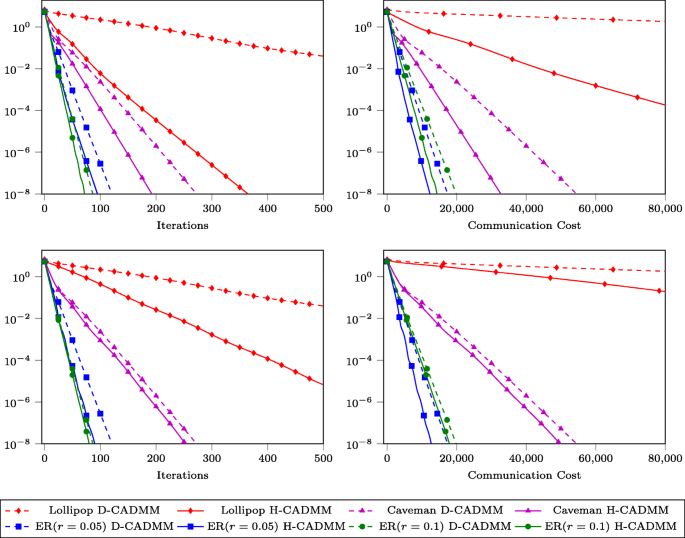
Performance comparison of D-CADMM and H-CADMM in terms of iteration number as well as communication cost. H-CADMM is configured with one dedicated FC connecting 50% of the nodes (top row figures) and 20% of the nodes, respectively (bottom row figures)
-
The tests verify the linear convergence properties of both D-CADMM and H-CADMM, as can be seen in all four graphs.
-
The performance gap between dashed lines and solid lines of the same marker confirms the acceleration ability of H-CADMM. The gap is larger for “badly connected” graphs, such as the lollipop graph and relatively small for “well-connected” graphs, such as the Erdős Rényi graphs. In fact, this observation holds even when comparing the Erdős Rényi graphs. Indeed, for the ER(r=0.05) graph which is not as well connected as the ER(r=0.1), the performance gap is smaller.
-
Figure 5 suggests that the more nodes are connected to the FC, the larger the acceleration gains for H-CADMM, which is intuitively reasonable since extra connections pay off. In view of this connections-versus-acceleration trade-off, H-CADMM can reach desirable sweet spots between performance gains and deployment cost.

6.3 In-network acceleration
In this test, we demonstrate the performance gain effected by in-network acceleration. By creating virtual FCs among nodes, this technique does not require dedicated FCs and new links. As detailed in Section 5, in-network accelerated H-CADMM exchanges information along existing edges, essentially leading to a communication cost that follows the same pattern with iteration complexity. Therefore, in this experiment, we report both metrics in one figure.
We first apply H-CADMM with in-network acceleration to several fixed-topology graphs, namely the line graph, the cycle graph, and the star graph, and we report the results in Fig. 6. Then, we carry out the same tests on the lollipop graph, the caveman graph and the two Erdos-Renyi graphs with parameters r=0.05 and r=0.10, and we present the results in Fig. 7. In each test, we select the hosts using Algorithm 2.

Effects of in-network acceleration on the line graph, the cycle graph, and the star graph

Effects of in-network acceleration on the lollipop graph, the caveman graph, and two Erdős Rényi random graphs
All the results illustrate that H-CADMM with in-network acceleration offers a significant boost in convergence rate over D-CADMM, especially for graphs with relatively large diameters (or graphs that are not well connected), such as the line graph, the cycle graph, or the lollipop graph. On the other hand, the performance gain is minimal for the star graph, whose diameter is 2 regardless of the number of nodes, as well as the Erdős Rényi random graph with high edge probability (see Fig. 7). Note that these performance gains over D-CADMM are achieved without paying a substantial computational cost (just one averaging step), which speaks for the practical merits of H-CADMM.
6.4 Trade-off between FCs and performance gain
Finally, we explore the trade-off between the number of LFCs and the corresponding convergence rate. We perform tests on several graphs with different properties and using only H-CADMM with in-network acceleration. In this test, we measure performance by the number of iterations needed to achieve a target accuracy of 10−8, given a varying number of LFCs ranging from 1 to 25.
Figure 8 depicts the results. In general, as the number of LFCs increases, the number of iterations decreases. Besides this general trend, one can also make the following observations.
-
For Erdős Rényi graphs with a relatively high-edge probability, there is a small initial gain arising from the introduction of virtual LFCs, which diminishes fast as their number increases. This is not surprising since such graphs are “well connected,” and therefore, adding more virtual LFCs does not help much. On the other hand, for “badly connected” graphs, such as the line graph or the lollipop graph, there is a significant convergence boost as the number of LFCs increases.
Fig. 8 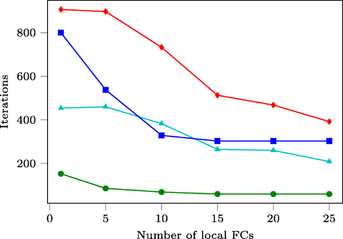
The impact of adding LFCs in H-CADMM with in-network acceleration. The performance is measured in terms of number of iterations needed to achieve certain accuracy
-
For the line and the cycle graph, a significant change in convergence rate happens only after an initial threshold has been surpassed (in our case 5–6 LFCs). For the lollipop graph, there seems to exist a cutoff point above which adding more nodes does not lead to significant change in convergence rate.

7 Conclusion and future work
This paper introduces the novel H-CADMM algorithm that generalizes the centralized and the decentralized CADMM, while also accelerating D-CADMM with modified updates.
We establish linear convergence of H-CADMM, and we also conduct a comprehensive set of numerical tests that validate our analytical findings and demonstrate the effectiveness of the proposed approach in practice.
A very promising direction we are currently pursuing involves the development of techniques leveraging the intrinsic hierarchical organization that is commonly found in distributed system architectures (see, e.g., [42, 43]) as well as real-world large-scale network topologies (see, e.g., [44, 45]).
8 Appendix A: Algorithm 1 for l>2
For l≥2, we have \({\mathbf {x}} \in \mathbb {R}^{Nl}\), \({\mathbf {z}}{} \in \mathbb {R}^{Ml}\), \({\boldsymbol {\lambda }} \in \mathbb {R}^{Tl}\), and \( {\mathbf {y}} \in \mathbb {R}^{Nl} \). Let \({\tilde {\mathbf {{A}}}} \in \mathbb {R}^{Tl\times Nl}\) and \({\tilde {\mathbf {{B}}}}\in \mathbb {R}^{Tl\times {}Ml}\) denote the coefficient matrices for l≥2, obtained by replacing 1’s of A and B with the identity matrix Il and 0’s with all-zero matrix 0l×l. Consequently, node degree, edge degree, and incidence matrices are \( {\tilde {\mathbf {{D}}}} = {\tilde {\mathbf {{A}}}}^{\top } {\tilde {\mathbf {{A}}}} \in \mathbb {R}^{Nl\times Nl}\), \( {\tilde {\mathbf {{E}}}} = {\tilde {\mathbf {{B}}}}^{\top } {\tilde {\mathbf {{B}}}} \in \mathbb {R}^{Ml\times Ml}\), and \({\tilde {\mathbf {{C}}}} = {\tilde {\mathbf {{A}}}}^{\top } {\tilde {\mathbf {{B}}}} \in \mathbb {R}^{Nl\times Ml}\). Meanwhile, H-CADMM boils down to
Relative to (13)–(15), the computational complexity of (39) is clearly higher. To see this, consider the per-step complexity for l=1. Given that E is a diagonal matrix, naive matrix-vector multiplication incurs complexity \({\mathcal {O}({MN})}\), which can be reduced to \({\mathcal {O}({M {E_{\text {max}}}})}\) by exploiting the sparsity of C, where Emax is the largest edge degree. When l≥2 however, per-step complexity grows to \( {\mathcal {O}({l^{2}M{E_{\text {max}}}})} \) which—being quadratic in l—would make it difficult for the method to handle high-dimensional data. Thankfully, a compact form of (39) made possible by Proposition 3 reduces the complexity from quadratic to linear in l.
Proposition 3
Let \({\mathbf {X}} \in {\mathbb {{R}}}^{N\times l}\) denote the matrix formed with ith row \({\mathbf {x}}_{i}^{\top }\) and likewise for \({\mathbf {Z}}\in {\mathbb {{R}}}^{M\times l} \) and \({\mathbf {Y}}\in {\mathbb {{R}}}^{N\times l}\). Then, (39) is equivalent to
Proof
The block structure suggests the following compact representation using Kronecker products
Exploiting properties of Kronecker products ([46], §2.8) matrices P, Q, R, and S with compatible dimensions satisfy
where x is obtained by concatenating all rows of X that we denote as x=vec(X⊤). Thus, by setting P=C and Q=Id, one arrives at
from which one readily obtains (40a) and (40c). To see the equivalence of (39b) and (40b), we use another property of Kronecker products, namely
Since \({\tilde {\mathbf {{E}}}}\) is block diagonal, so is \( {\tilde {\mathbf {{E}}}}^{-1} = {\mathbf {E}}^{-1}\otimes {\mathbf {I}}_{d} \). Therefore, (39b) is equivalent to
which concludes the proof. □
Proposition 3 establishes that H-CADMM can run using much smaller matrices, effectively reducing its computational complexity. To see this, consider the per-step complexity of (40). The difference with (39) is dominated by
C⊤X, which leads to complexity \({\mathcal {O}({lMN})}\). This can be further reduced to \({\mathcal {O}({lM{E_{\text {max}}}})}\) by exploiting the sparsity of C, thus improving the complexity of (39) by a factor of l.
9 Proof of Lemma 1
Let ai denote the ith column of A, and bj the jth column of B. By construction, the ith column of A indicates in which constraint xi is present; hence, \( {{\mathbf {{a}}}}_{i}^{{\top }}{{\mathbf {{a}}}}_{i} = d_{i}\) equals the degree of node i. Similarly, it follows that \({{\mathbf {{b}}}}_{j}^{{\top }}{{\mathbf {{b}}}_{j}} = {e_{j}}\), and
from which we obtain A⊤A=D and B⊤B=E.
Consider now the dot product \({{\mathbf {{a}}}}_{i}^{\top }{{\mathbf {{b}}}_{j}}\). When the tth constraint reads xi=zj, it holds by construction that (ai)t=1, and (bj)t=1. Therefore, if node i and edge j are incident, we have \({{\mathbf {{a}}}}_{i}^{\top }{{\mathbf {{b}}}_{j}} = 1\); otherwise, \({{\mathbf {{a}}}}_{i}^{\top }{{\mathbf {{b}}}_{j}} = 0\). Thus, the incidence matrix definition implies that A⊤B=C.
10 Proof of Lemma 3
Let emax (emin) denote the maximum (minimum) degree of all edges, and cij the number of common edges between nodes i and j. Clearly, we have \(d_{i} = \sum _{j=1}^{N} c_{ij}\), with cii=0; and since E≼emaxI, we obtain
where the last inequality holds because C has linearly independent columns, and hence CC⊤ is PSD. The latter implies that CE−1C⊤ is PSD too.
The definition of C leads to
And since E≽emin I, it holds that
where the last matrix is a valid Laplacian (\(d_{i} = \sum _{j=1}^{N} c_{ij}\)), which in turn implies that it is PSD.
Finally, by definition C1=d, C⊤1=e, where d:=[d1,…,dN]⊤, e:=[e1,…,eN]⊤; and hence we have
11 Proof of Lemma 4
Feasibility of (25c) guarantees the existence of at least one solution, and therefore, there exists at least one optimal solution. The uniqueness of x⋆ and z⋆ follows from the strong convexity of F(·) and the dual feasibility (25c).
To see the uniqueness of y, we first show that if \( \tilde {{\boldsymbol {\lambda }}} \) is optimal, then λ⋆, the projection of \(\tilde {{\boldsymbol {\lambda }}}\) to the column space of A, is also optimal. Using the orthogonality principle, we arrive at
which implies that λ⋆ also satisfies (25a). Thus, projection of any solution \( \tilde {{\boldsymbol {\lambda }}} \) to the column space of A is also an optimal solution.
If there are two optimal solutions, λ1≠λ2 in the column space of A, we have
Furthermore, there exist x1≠x2 such that λ1=Ax1 and λ2=Ax2. Subtracting A⊤λ2 from A⊤λ1 yields
from which we find that x1=x2, which is a contradiction. Therefore, λ1=λ2, and thus, y=A⊤λ is also unique.
12 Proof of Lemma 5
To simplify the notation, let S:=CE−1C⊤. Using Lemma 2, we arrive at
Subtracting (D−S)xk+1 from both sides yields
Noticing that Q=(D−S)1/2 and \( {\mathbf {r}}^{k} = \sum _{t=0}^{k}{\mathbf {Qx}}^{t} \), we obtain
The proof of Lemma 2 shows that if y0=0, then yk=ρQrk, which leads to y⋆=ρQr⋆ as k→∞. Using (25), we arrive at
Combining this with (43) completes the proof.
13 Proof of Theorem 1
It suffices to prove that
Lemma 5 and the strong convexity of F(·) lead to
Similarly, Lemma 5 and strong convexity imply that
For any β∈(0,1), we have
To prove (44), it suffices to show that
which is equivalent to
where \( {\mathbf {M}} := \frac {2{\sigma }\beta }{{\rho }}{\mathbf {I}} - \delta {\mathbf {CE}}^{-1}{\mathbf {C}}^{\top } \). Observing the left hand side of (45), it suffices to show that
Since rk+1 and r⋆ are orthogonal to 1 and the null space of Q is span {1}, both vectors belong to the column space of Q. Using Lemma 4, we obtain
Comparing (47) with (46) suggests that it is sufficient to have
Notes
This should be expected since H-CADMM reduces to D-CADMM upon modeling each simple edge as an hyperedge.
References
L. Xiao, S. Boyd, S. Lall, in Proceedings of the 4th International Symposium on Information Processing in Sensor Networks. IPSN ’05. A scheme for robust distributed sensor fusion based on average consensus (IEEELos Angeles, 2005), pp. 63–70.
R. Olfati-Saber, in Proceedings of the 44th IEEE Conference on Decision and Control. Distributed Kalman Filter with Embedded Consensus Filters (IEEESeville, 2005), pp. 8179–8184.
Q. Ling, Z. Tian, Decentralized sparse signal recovery for compressive sleeping wireless sensor networks. IEEE Trans. Signal Process.58(7), 3816–3827 (2010).
I. D. Schizas, A. Ribeiro, G. B. Giannakis, Consensus in ad hoc WSNs with noisy links—part I: distributed estimation of deterministic signals. IEEE Trans. Signal Process.56(1), 350–364 (2008).
W. Ren, R. W. Beard, E. M. Atkins, Information consensus in multivehicle cooperative control. IEEE Control Syst. Mag.27(2), 71–82 (2007).
W. Ren, in 2006 American Control Conference. Consensus based formation control strategies for multi-vehicle systems (Minneapolis, 2006), pp. 4237–4242.
V. Kekatos, G. B. Giannakis, Distributed robust power system state estimation. IEEE Trans. Power Syst.28(2), 1617–1626 (2013).
P. A. Forero, A. Cano, G. B. Giannakis, Distributed clustering using wireless sensor networks. IEEE J. Sel. Top. Signal Process.5(4), 707–724 (2011).
P. A. Forero, A. Cano, G. B. Giannakis, Consensus-based distributed support vector machines. J. Mach. Learn. Res.11(May), 1663–1707 (2010).
G. Mateos, J. A. Bazerque, G. B. Giannakis, Distributed sparse linear regression. IEEE Trans. Signal Process.58(10), 5262–5276 (2010).
R. Olfati-Saber, J. S. Shamma, in Proceedings of the 44th IEEE Conference on Decision and Control. Consensus Filters for Sensor Networks and Distributed Sensor Fusion (IEEESeville, 2005), pp. 6698–6703.
H. Zhu, A. Cano, G. Giannakis, Distributed consensus-based demodulation: algorithms and error analysis. IEEE Trans. Wirel. Commun.9(6), 2044–2054 (2010).
J. A. Bazerque, G. B. Giannakis, Distributed spectrum sensing for cognitive radio networks by exploiting sparsity. IEEE Trans. Signal Process.58(3), 1847–1862 (2010).
D. P. Bertsekas, J. N. Tsitsiklis, Parallel and distributed computation: numerical methods vol. 23 (Prentice-Hall, Inc., Upper Saddle River, 1989).
S. Boyd, N. Parikh, E. Chu, B. Peleato, J. Eckstein, Distributed optimization and statistical learning via the alternating direction method of multipliers. Found. Trends® Mach. Learn.3(1), 1–122 (2011).
T. Erseghe, D. Zennaro, E. Dall’Anese, L. Vangelista, Fast consensus by the alternating direction multipliers method. IEEE Trans. Signal Process.59(11), 5523–5537 (2011).
T. Goldstein, B. O’Donoghue, S. Setzer, R. Baraniuk, Fast alternating direction optimization methods. SIAM J. Imaging Sci.7(3), 1588–1623 (2014).
M. Hong, Z. -Q. Luo, On the linear convergence of the alternating direction method of multipliers. Math. Program.162(1-2), 165–199 (2017).
W. Deng, W. Yin, On the global and linear convergence of the generalized alternating direction method of multipliers. J Sci Comput. 66(3), 889–916 (2015).
G. B. Giannakis, Q. Ling, G. Mateos, I. D. Schizas, H. Zhu, in Splitting Methods in Communication, Imaging, Science, and Engineering, ed. by R. Glowinski, S. J. Osher, and W. Yin. Decentralized learning for wireless communications and networking (Springer International PublishingCham, 2016), pp. 461–497.
W. Shi, Q. Ling, K. Yuan, G. Wu, W. Yin, On the linear convergence of the ADMM in decentralized consensus optimization. IEEE Trans. Signal Process.62(7), 1750–1761 (2014).
J. N. Tsitsiklis, Problems in Decentralized Decision Making and Computation (Massachusetts Institute of Technology, Cambridge, 1984).
A. Nedic, A. Ozdaglar, Distributed subgradient methods for multi-agent optimization. IEEE Trans. Autom. Control. 54(1), 48–61 (2009).
A. Nedic, A. Ozdaglar, P. A. Parrilo, Constrained consensus and optimization in multi-agent networks. IEEE Trans. Autom. Control. 55(4), 922–938 (2010).
H. Terelius, U. Topcu, R. M. Murray, Decentralized multi-agent optimization via dual decomposition. IFAC Proc. Vol.44(1), 11245–11251 (2011).
K. I. Tsianos, M. G. Rabbat, in 50th Annual Allerton Conference on Communication, Control, and Computing (Allerton). Distributed strongly convex optimization (IEEEMonticello, 2012), pp. 593–600.
S. Sundhar Ram, A. Nedić, V. V. Veeravalli, Distributed Stochastic Subgradient Projection Algorithms for Convex Optimization. J. Optim. Theory. Appl.147(3), 516–545 (2010).
JC Duchi, A Agarwal, MJ Wainwright, Dual averaging for distributed optimization: convergence analysis and network scaling. IEEE Trans. Autom. Control.57(3), 592–606 (2012).
K. Tsianos, S. Lawlor, M. G. Rabbat, in Advances in Neural Information Processing Systems 25, ed. by F. Pereira, C. J. C. Burges, L. Bottou, and K. Q. Weinberger. Communication/Computation Tradeoffs in Consensus-Based Distributed Optimization (Curran Associates, Inc.New York, 2012), pp. 1943–1951.
A. G. Dimakis, S. Kar, J. M. F. Moura, M. G. Rabbat, A. Scaglione, Gossip algorithms for distributed signal processing. Proc. IEEE. 98(11), 1847–1864 (2010).
A. Makhdoumi, A. Ozdaglar, Convergence rate of distributed ADMM over networks. IEEE Trans. Autom. Control. 62(10), 5082–5095 (2017).
R. Glowinski, A. Marroco, Sur l’approximation, par éléments finis d’ordre un, et la résolution, par pénalisation-dualité d’une classe de problèmes de Dirichlet non linéaires. Rev. Fr. Autom. Inform. Rech. Opérationnelle Anal. Numér.9(R2), 41–76 (1975).
D. Gabay, in Studies in Mathematics and Its Applications. Augmented Lagrangian Methods: Applications to the Numerical Solution of Boundary-Value Problems, vol. 15, ed. by M. Fortin, R. Glowinski. Applications of the method of multipliers to variational inequalities (North-Holland, Amsterdam, 1983), pp. 299–331.
J. Eckstein, D. P. Bertsekas, On the Douglas–Rachford splitting method and the proximal point algorithm for maximal monotone operators. Math. Program.55(1-3), 293–318 (1992).
D. Boley, Local linear convergence of the alternating direction method of multipliers on quadratic or linear programs. SIAM J. Optim.23(4), 2183–2207 (2013).
J. A. Bazerque, G. Mateos, G. B. Giannakis, Group-Lasso on splines for spectrum cartography. Signal Process. IEEE Trans. On. 59(10), 4648–4663 (2011).
Q. Ling, Y. Liu, W. Shi, Z. Tian, in 2016 IEEE International Conference on Acoustics, Speech and Signal Processing. Communication-efficient weighted ADMM for decentralized network optimization (IEEEShanghai, 2016), pp. 4821–4825.
J. B. Predd, S. R. Kulkarni, H. V. Poor, A collaborative training algorithm for distributed learning. IEEE Trans. Inf. Theory. 55(4), 1856–1871 (2009).
F. Iutzeler, P. Bianchi, P. Ciblat, W. Hachem, Explicit convergence rate of a distributed alternating direction method of multipliers. IEEE Trans. Autom. Control. 61(4), 892–904 (2016).
M. Ma, A. N. Nikolakopoulos, G. B. Giannakis, in Proceedings of 2018 IEEE International Conference on Acoustics, Speech, and Signal Processing (ICASSP). Fast decentralized learning via hybrid consensus ADMM (IEEECalgary, 2018).
F. R. K. Chung, Spectral Graph Theory vol. no. 92 (American Mathematical Society, Providence, R.I, 1997).
J. P. Gross, R. B. Pandit, C. G. Cook, T. H. Matson, Network with distributed shared memory. US9317469B2: (2016).
A. N. Nikolakopoulos, J. D. Garofalakis, in Proceedings of the 2016 PCI Conference. PCI ’16. On the multi-level near complete decomposability of a class of multiprocessing systems (ACMNew York, 2016), pp. 14–1146.
M. Faloutsos, P. Faloutsos, C. Faloutsos, in Proceedings of the Conference on Applications, Technologies, Architectures, and Protocols for Computer Communication, SIGCOMM ’99. On power-law relationships of the internet topology (ACMNew York, 1999), pp. 251–262.
M. E. Newman, The structure and function of complex networks. SIAM Rev. 45(2), 167–256 (2003).
A. K. Jain, Fundamentals of Digital Image Processing (Prentice-Hall, Inc., Upper Saddle River, 1989).
Acknowledgements
The authors wish to thank Prof. M. Hong from University of Minnesota for insightful discussions on related subjects. Part of this work was supported by NSF grants 1442686, 1500713, 1509040, and 171141.
Author information
Authors and Affiliations
Contributions
All authors read and approved the final manuscript.
Corresponding author
Ethics declarations
Competing interests
The authors declare that they have no competing interests.
Publisher’s Note
Springer Nature remains neutral with regard to jurisdictional claims in published maps and institutional affiliations.
Rights and permissions
Open Access This article is distributed under the terms of the Creative Commons Attribution 4.0 International License (http://creativecommons.org/licenses/by/4.0/), which permits unrestricted use, distribution, and reproduction in any medium, provided you give appropriate credit to the original author(s) and the source, provide a link to the Creative Commons license, and indicate if changes were made.
About this article

Cite this article
Ma, M., Nikolakopoulos, A.N. & Giannakis, G.B. Hybrid ADMM: a unifying and fast approach to decentralized optimization. EURASIP J. Adv. Signal Process. 2018, 73 (2018). https://doi.org/10.1186/s13634-018-0589-x
Received:
Accepted:
Published:
DOI: https://doi.org/10.1186/s13634-018-0589-x