
Abstract
Without the strong monotonicity assumption of the mapping, we provide a regularization method for general variational inequality problem, when its solution set is related to a solution set of an inverse strongly monotone mapping. Consequently, an iterative algorithm for finding such a solution is constructed, and convergent theorem of the such algorithm is proved. It is worth pointing out that, since we do not assume strong monotonicity of general variational inequality problem, our results improve and extend some well-known results in the literature.
1. Introduction
It is well known that the ideas and techniques of the variational inequalities are being applied in a variety of diverse fields of pure and applied sciences and proven to be productive and innovative. It has been shown that this theory provides the most natural, direct, simple, unified, and efficient framework for a general treatment of a wide class of linear and nonlinear problems. The development of variational inequality theory can be viewed as the simultaneous pursuit of two different lines of research. On the one hand, it reveals the fundamental facts on the qualitative aspects of the solutions to important classes of problems. On the other hand, it also enables us to develop highly efficient and powerful new numerical methods for solving, for example, obstacle, unilateral, free, moving, and complex equilibrium problems.
In 1988, Noor [1] introduced and studied a class of variational inequalities, which is known as general variational inequality, GVI K (A, g), is as follows: Find u* ∈ H, g(u*) ∈ K such that

where K is a nonempty closed convex subset of a real Hilbert space H with inner product 〈·, ·〉, and T, g: H → H be mappings. It is known that a class of nonsymmetric and odd-order obstacle, unilateral, and moving boundary value problems arising in pure and applied can be studied in the unified framework of general variational inequalities (e.g., [2] and the references therein). Observe that to guarantee the existence and uniqueness of a solution of the problem (1.1), one has to impose conditions on the operator A and g, see [3] for example in a more general case. By the way, it is worth noting that, if A fails to be Lipschitz continuous or strongly monotone, then the solution set of the problem (1.1) may be an empty one.
Related to the variational inequalities, we have the problem of finding the fixed points of the nonlinear mappings, which is the subject of current interest in functional analysis. It is natural to consider a unified approach to these two different problems (e.g., [3–8]). Motivated and inspired by the research going in this direction, in this article, we present a method for finding a solution of the problem (1.1), which is related to the solution set of an inverse strongly monotone mapping and is as follows: Find u* ∈ H, g(u*) ∈ S(T) such that

when A is a generalized monotone mapping, T: K → H is an inverse strongly monotone mapping, and S(T) = {x ∈ K: T(x) = 0}. We will denote by GVI K (A, g, T) for a set of solution to the problem (1.2). Observe that, if T =: 0, the zero operator, then the problem (1.2) reduces to (1.1). Moreover, we would also like to notice that although many authors have proven results for finding the solution of the variational inequality problem and the solution set of inverse strongly monotone mapping (e.g., [4, 8, 9]), it is clear that it cannot be directly applied to the problem GV I K (A, g, T) due to the presence of g.
2. Preliminaries
Let H be a real Hilbert space whose inner product and norm are denoted by 〈·, ·〉 and || · ||, respectively. Let K be a nonempty closed convex subset of H. In this section, we will recall some well-known results and definitions.
Definition2.1. Let A: H → H be a mapping and K ⊂ H. Then, A is said to be semi-continuous at a point x in K if

Definition2.2. A mapping T: K → H is said to be λ-inverse strongly monotone, if there exists a λ > 0 such that

Recall that a mapping B: K → H is said to be k-strictly pseudocontractive if there exists a constant k ∈ [0, 1) such that

Let I be the identity operator on K. It is well known that if B: K → H is a k-strictly pseudocontrative mapping, then the mapping T := I - B is a  -inverse strongly monotone, see [4]. Conversely, if T: K → H is a λ-inverse strongly monotone with
  , then B := I - T is (1 - 2λ)-strictly pseudocontrative mapping. Actually, for all x, y ∈ K, we have

On the other hand, since H is a real Hilbert space, we have

Hence,

Moreover, we have the following result:
Lemma 2.3. [10]Let K be a nonempty closed convex subset of a Hilbert space H and B: K → H a k-strictly pseudocontractive mapping. Then, I - B is demiclosed at zero, that is, whenever {x n } is a sequence in K such that {x n } converges weakly to x ∈ K and {(I - B)(x n )} converges strongly to 0, we must have (I - B)(x) = 0.
Definition2.4. Let A, g: H → H. Then A is said to be g-monotone if

For g = I, the identity operator, Definition 2.4 reduces to the well-known definition of monotonicity. However, the converse is not true.
Now we show an example in proof of our main problem (1.2).
Example 2.5. Let a, b be strictly positive real numbers. Put H = {(x1, x2)| -a ≤ x1 ≤ a, -b ≤ x2 ≤ b} with the usual inner product and norm. Let K = {(x1, x2) ∈ H: 0 ≤ x1 ≤ x2} be a closed convex subset of H. Let T: K → H be a mapping defined by T(x) = (I - PΔ)(x), where Δ = {x := (x1, x2) ∈ H: x1 = x2} is a closed convex subset of H, and PΔ is a projection mapping from K onto Δ. Clearly, T is  -inverse strongly monotone, and S(T) = Δ ∩ K. Now, if
  is a considered matrix operator and g = -I, where I is the 2 × 2 identity matrix. Then, we can verify that A is a g-monotone operator. Indeed, for each x := (x1, x2), y := (y1, y2) ∈ H, we have

Moreover, if  , then we must have 〈A(u*), g(y) - g(u*)〉 ≥ 0, for all y = (y1, y2) ∈ H, g(y) ∈ K. This equivalence becomes

for all y = (y1, y2) ∈ H, g(y) ∈ K. Notice that g-1(K) = {(y1, y2) ∈ H|y1 ≥ y2}. Thus, in view of (2.1), it follows that {x = (x1, x2) ∈ H|x1 = x2} ⊂ GVI K (A, g). Hence, GVI K (A, g, T) ≠ ∅.
Remark 2.6. In Example 2.5, the operator A is not a monotone mapping on H.
We need the following concepts to prove our results.
Let  stand for the set of real numbers. Let
  be an equilibrium bifunction, that is, F(u, u) = 0 for every u ∈ K.
Definition2.7. The equilibrium bifunction is said to be
(i) monotone, if for all u, v ∈ K, then we have

(ii) strongly monotone with constant τ; if for all u, v ∈ K, then we have

(iii) hemicontinuous in the first variable u; if for each fixed v, then we have

Recall that the equilibrium problem for is to find u* ∈ K such that

Concerning to the problem (2.5), the following facts are very useful.
Lemma 2.8. [11]Letbe such that F(u, v) is convex and lower semicontinuous in the variable v for each fixed u ∈ K. Then,
-
(1)
if F(u, v) is hemicontinuous in the first variable and has the monotonic property, then U* = V*, where U* is the solution set of (2.5), and V* is the solution set of F(u, v*) ≤ 0 for all u ∈ K. Moreover, in this case, they are closed and convex;
-
(2)
if F(u, v) is hemicontinuous in the first variable for each v ∈ K and F is strongly monotone, then U* is a nonempty singleton. In addition, if F is a strongly monotone mapping, then U* = V* is a singleton set.
The following basic results are also needed.
Lemma 2.9. Let {x n } be a sequence in H. If x n → x wealky and ||x n || → ||x||, then x n → x strongly.
Lemma 2.10. [12]. Let a n , b n , c n be the sequences of positive real numbers satisfying the following conditions.
(i) an+1≤ (1 - b n )a n + c n , b n < 1,
(ii)  .
.
Then, limn→+∞a n = 0.
3. Regularization
Let α ∈ (0, 1) be a fixed positive real number. We now construct a regularization solution u α for (1.2), by solving the following general variational inequality problem: find u α ∈ H, g(u α ) ∈ K such that

Theorem 3.1. Let K be a closed convex subset of a Hilbert space H and g: H → H be a mapping such that K ⊂ g(H). Let A: H → H be a hemicontinuous on K and g-monotone mapping, T: K → H be λ-inverse strongly monotone mapping. If g is an expanding affine continuous mapping and GVI K (A, g, T) ≠ ∅, then the following conclusions are true.
-
(a)
For each α ∈ (0, 1), the problem (3.1) has the unique solution u α :
-
(b)
If α ↓ 0, then {g(u α )} converges. Moreover,
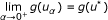 for some u* ∈ GVI
K
(A, g, T).
for some u* ∈ GVI
K
(A, g, T). -
(c)
There exists a positive constant M such that
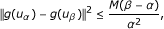 (3.2)
(3.2)
 for some u* ∈ GVI
K
(A, g, T).
for some u* ∈ GVI
K
(A, g, T).
when 0 < α < β < 1.
Proof. First, in view of the definition 2.2, we will always assume that . Now, related to mappings A, T, and g, we define functions  by
by

for all (u, v) ∈ g-1(K) × g-1(K). Note that, F A , F T are equilibrium monotone bifunctions, and g-1(K) is a closed convex subset of H.
Now, let α ∈ (0, 1) be a given positive real number. We construct a function  by
by

for all (u, v) ∈ g-1(K) × g-1(K).
-
(a)
Observe that, the problem (3.1) is equivalent to the problem of finding u α ∈ g -1(K) such that
 (3.4)
(3.4)

Moreover, one can easily check that F α (u, v) is a monotone hemicontinuous in the variable u for each fixed v ∈ g-1(K). Indeed, it is strongly monotone with constant αξ > 0, where g is an ξ-expansive. Thus, by Lemma 2.8(ii), the problem (3.4) has a unique solution u α ∈ g-1(K) for each α > 0. This prove (a).
-
(b)
Note that for each y ∈ GVI K (A, g, T) we have [F A + αμF T ](y, u α ) ≥ 0. Consequently, by (3.4), we have


This means

Consequently,

that is, ||g(u
α
)|| ≤ ||g(y)|| for all y ∈ GVI
K
(A, g, T). Thus, {g(u
α
)} is a bounded subset of K. Consequently, the set of weak limit points as α → 0 of the net (g(u
α
)) denoted by ω
w
(g(u
α
)) is nonempty. Pick z ∈ ω
w
(g(u
α
)) and a null sequence {α
k
} in the interval (0, 1) such that  weakly converges to z as k → ∞. Since K is closed and convex, we know that K is weakly closed, and it follows that z ∈ K. Now, since K ⊂ g(H), we let u* ∈ H be such that z = g(u*) and claim that u* ∈ GVI
K
(A, g, T).
weakly converges to z as k → ∞. Since K is closed and convex, we know that K is weakly closed, and it follows that z ∈ K. Now, since K ⊂ g(H), we let u* ∈ H be such that z = g(u*) and claim that u* ∈ GVI
K
(A, g, T).
To prove such a claim, we will first show that g(u*) ∈ S(T). To do so, let us pick a fixed y ∈ GVI K (A, g, T). By (3.3) and the monotonicity of F A , we have

equivalently,

for each k ∈ ℕ. Using the above together with the assumption that T is an λ-inverse strongly monotone mapping, we have

for each k ∈ ℕ. Letting k → +∞, we obtain

On the other hand, we know that the mapping I - T is a strictly pseudocontractive, thus by lemma 2.3, we have T demiclosed at zero. Consequently, since weakly converges to g(u*), we obtain T(g(u*)) = T(g(y)) = 0. This proves g(u*) ∈ S(T), as required.
Now, we will show that u* ∈ GVI K (A, g, T). Notice that, from the monotonic property of F α and (3.4), we have

for all v ∈ g-1(K). That is,

for all v ∈ g-1(K). Since α k ↓ 0 as k → ∞, we see that (3.6) implies F A (v, u*) ≤ 0 for any v ∈ H, g(v) ∈ K. Consequently, in view of Lemma 2.8(1), we obtain our claim immediately.
Next we observe that the sequence actually converges to g(u*) strongly. In fact, by using a lower semi-continuous of norm and (3.5), we see that

since u* ∈ GVI
K
(A, g, T). That is,  as k → ∞. Now, it is straight-forward from Lemma 2.9, that the weak convergence to g(u*) of implies strong convergence to g(u*) of . Further, in view of (3.5), we see that

Next, we let  , where {α
j
} be any null sequence in the interval (0, 1). By following the lines of proof as above, and passing to a subsequence if necessary, we know that there is
, where {α
j
} be any null sequence in the interval (0, 1). By following the lines of proof as above, and passing to a subsequence if necessary, we know that there is  such that
  as j → ∞. Moreover, in view of (3.5) and (3.7), we have
  . Consequently, since the function ||g(·)|| is a lower semi-continuous function and GVI
K
(A, g, T) is a closed convex set, we see that (3.7) gives
. Consequently, since the function ||g(·)|| is a lower semi-continuous function and GVI
K
(A, g, T) is a closed convex set, we see that (3.7) gives  . This has shown that g(u*) is the strong limit of the net (g(u
α
)) as α ↓ 0.
. This has shown that g(u*) is the strong limit of the net (g(u
α
)) as α ↓ 0.
-
(c)
Let 0 < α < β < 1 and u α , u β are solutions of the problem (3.1). Thus, since F A and F T are monotone mappings, by (3.4), we have


that is,

Notice that,

since 0 < α < β. Using the above, by (3.8), we have

where θ = sup{||g(u
α
)||: α ∈ (0, 1)}. Moreover, since F
T
is a Lipschit continuous mapping (with Lipschitz constant  ), it follows that

for some M1 > 0. Further, by applying the Lagranges mean-value theorem to a continuous function h(t) = t-μon [1, +∞), we know that

for some M > 0. This completes the proof. □
Remark 3.2. If g =: I, the identity operator on H, then we see that Theorem 3.1 reduces to a result presented by Kim and Buong [9].
4. Iterative Method
Now, we consider the regularization inertial proximal point algorithm:

The well definedness of (4.1) is guaranteed by the following result.
Proposition 4.1. Assume that all hypothesis of the Theorem 3.1 are satisfied. Let z ∈ g-1(K) be a fixed element. Define a bifunction F z : g-1(K) × g-1(K) → ℝ by

where c, α are positive real numbers. Then, there exists the unique element u* ∈ g-1(K) such that F z (u*, v) ≥ 0 for all v ∈ g-1(K).
Proof. Assume that g is an ξ- expanding mapping. Then, for each u, v ∈ g-1(K), we see that

This means F is ξ(1 + cα)-strongly monotone. Consequently, by Lemma 2.8, the proof is completed. □
The result of the next theorem shows some sufficient conditions for the convergent of regularization inertial proximal point algorithm (4.1).
Theorem 4.2. Assume that all the hypotheses of the Theorem 3.1 are satisfied. If the parameters c n and α n are chosen as positive real numbers such that
(C1)  ,
,
(C2)  ,
,
(C3)  ,
,
then the sequence {g(z n )} defined by (4.1) converges strongly to the element g(u*) as n → +∞, where u* ∈ GVI K (A, g, T).
Proof. From (4.1) we have

that is

or equivalently,

so

Hence

where

On the other hand, by Theorem 3.1, there is u n ∈ g-1(K) such that

for all n ∈ ℕ. This implies

and so

Thus,

By setting v = u n in (4.2) we have

and v = zn+1in (4.4) we have

and adding one obtained result to the other, we get

Notice that, since A is a g-monotone mapping, and T is a λ-inverse strongly monotone, we have

and

Thus, by (4.5), we obtain

that is,

Consequently,

which implies that

Using the above Equation 4.6 and (3.2), we know that

where

Consequently, by the condition (C3), we have  . Meanwhile, the conditions (C2) and (C3) imply that
  . Thus, all the conditions of Lemma 2.10 are satisfied, then it follows that ||g(zn+1) - g(un+1)|| → 0 as n → ∞. Moreover, by (C1) and Theorem 3.1, we know that there exists u* ∈ GVI
K
(A, g, T) such that g(u
n
) converges strongly to g(u*). Consequently, we obtain that g(z
n
) converges strongly to g(u*) as n → +∞. This completes the proof. □
. Thus, all the conditions of Lemma 2.10 are satisfied, then it follows that ||g(zn+1) - g(un+1)|| → 0 as n → ∞. Moreover, by (C1) and Theorem 3.1, we know that there exists u* ∈ GVI
K
(A, g, T) such that g(u
n
) converges strongly to g(u*). Consequently, we obtain that g(z
n
) converges strongly to g(u*) as n → +∞. This completes the proof. □
Remark 4.3. The sequences {α n } and {c n } which are defined by

satisfy all the conditions in Theorem 4.2.
Remark 4.4. It is worth noting that, because of condition (C2) of Theorem 4.2, the important natural choice {1/n} does not include in the class of parameters {α n }. This leads to a question: Can we find another regularization inertial proximal point algorithm for the problem (1.2) that includes a natural parameter choice {1/n}?
Remark 4.5. If F is a nonexpansive mapping, then I - F is an inverse strongly monotone mapping, and the fixed points set of mapping F and the solution set S(I - F) are equal. This means that our results contain the study of finding a common element of (general) variational inequalities problems and fixed points set of nonexpansive mapping, which were studied in [4–8] as special cases.
References
Noor MA: General variational inequalities. Appl Math Lett 1988, 1: 119–121. 10.1016/0893-9659(88)90054-7
Noor MA: Some developments in general variational inequalities. Appl Math Comput 2004, 152: 199–277. 10.1016/S0096-3003(03)00558-7
Petrot N: Existence and algorithm of solutions for general set-valued Noor variational inequalities with relaxed ( μ , ν )-cocoercive operators in Hilbert spaces. J Appl Math Comput 2010, 32: 393–404. 10.1007/s12190-009-0258-1
Iiduka H, Takahashi W: Strong convergence theorems for nonexpansive mappings and inverse-strongly monotone mappings. Nonlinear Anal 2005, 61: 341–350. 10.1016/j.na.2003.07.023
Noor MA: General variational inequalities and nonexpansive mappings. J Math Anal Appl 2007, 331: 810–822. 10.1016/j.jmaa.2006.09.039
Noor MA, Huang Z: Wiener-Hopf equation technique for variational inequalities and nonexpansive mappings. Appl Math Comput 2007, 191: 504–510. 10.1016/j.amc.2007.02.117
Qin X, Noor MA: General WienerHopf equation technique for nonexpansive mappings and general variational inequalities in Hilbert spaces. Appl Math Comput 2008, 201: 716–722. 10.1016/j.amc.2008.01.007
Takahashi W, Toyoda M: Weak convergence theorems for nonexpansive mappings and monotone mappings. J Optim Theory Appl 2003,118(2):417–428. 10.1023/A:1025407607560
Kim JK, Buong N: Regularization inertial proximal point algorithm for monotone hemicontinuous mapping and inverse strongly monotone mappings in Hilbert spaces. J Inequal Appl 2010, 10. Article ID 451916
Osilike MO, Udomene A: Demiclosedness principle and convergence theorems for strictly pseudo-contractive mappings of Browder-Petryshyn type. J Math Anal Appl 2001,256(2):431–445. 10.1006/jmaa.2000.7257
Blum E, Oettli W: From optimization and variational inequalities to equilibrium problems. Math Stud 1994, 63: 123–145.
Xu HK: Iterative algorithms for nonlinear operators. J Lond Math Soc 2002,66(1):240–256. 10.1112/S0024610702003332
Acknowledgements
YJC was supported by the Korea Research Foundation Grant funded by the Korean Government (KRF-2008-313-C00050). NP was supported by Faculty of Science, Naresuan University (Project No. R2553C222), and the Commission on Higher Education and the Thailand Research Fund (Project No. MRG5380247).
Author information
Authors and Affiliations
Corresponding author
Additional information
Competing interests
The authors declare that they have no competing interests.
Authors' contributions
Both authors contributed equally in this paper. They read and approved the final manuscript.
Rights and permissions
Open Access This article is distributed under the terms of the Creative Commons Attribution 2.0 International License (https://creativecommons.org/licenses/by/2.0), which permits unrestricted use, distribution, and reproduction in any medium, provided the original work is properly cited.
About this article
Cite this article
Cho, Y.J., Petrot, N. Regularization and iterative method for general variational inequality problem in hilbert spaces. J Inequal Appl 2011, 21 (2011). https://doi.org/10.1186/1029-242X-2011-21
Received:
Accepted:
Published:
DOI: https://doi.org/10.1186/1029-242X-2011-21