
Abstract
Performance gain achieved by adding mobile nodes to a stationary sensor network for target detection depends on factors such as the number of mobile nodes deployed, mobility patterns, speed and energy constraints of mobile nodes, and the nature of the target locations (deterministic or random). In this paper, we address the problem of distributed detection of a randomly located target by a hybrid sensor network. Specifically, we develop two decision-fusion architectures for detection where in the first one, impact of node mobility is taken into account for decisions updating at the fusion center, while in the second model the impact of node mobility is taken at the node level decision updating. The cost of deploying mobile nodes is analyzed in terms of the minimum fraction of mobile nodes required to achieve the desired performance level within a desired delay constraint. Moreover, we consider managing node mobility under given constraints.
1. Introduction
The problem of distributed detection and decision fusion in stationary wireless sensor networks has been extensively studied by many authors in different contexts [1–6]. However, stationary sensor networks may not suit for some applications, for example, in situations where it might be necessary to deploy a huge number of static nodes with limited coverage to monitor a large region within a desired performance level. In such situations, if relatively a small number of nodes are allowed to move, the system performance can be improved over time due to improvement in sensing coverage [7]. Deploying mobile nodes in a sensor network, however, may not be as cost-effective as deploying static nodes. Also, nodes will have to spend node energy for mobility in addition to sensing and communication. Thus, it is desirable to allow only a fraction of the nodes of the network to be mobile according to the requirement.
In this paper, we consider the problem of detecting a randomly located stationary target in a hybrid sensor network made of both mobile and static nodes. At the initial deployment stage, static and mobile nodes may scatter in the region of interest in random fashion, if the network does not have prior information about Phenomenon of Interest (PoI). Mobile nodes may be required to perform on-demand for different applications after the initial deployment. Due to energy constraints, we assume that the mobile nodes are kept stationary until a target is detected with certain confidence level, or useful statistics regarding the target locations are available. Note that since mobile nodes are required to perform on-demand for different functionalities, it is not possible to locate them in a certain area for a specific task. We assume that, at each time step, a mobile node can move to a limited number of locations from its current position, where these candidate locations are determined by physical factors related to mobile sensors and the environment. At each time step, mobile nodes move in a direction chosen based on the proposed mobility management schedule to maximize the detection probability during a desired delay constraint. At each time step, each node makes a local binary decision based on its observations and transmits it to the fusion center. The fusion center combines local decisions from all static and mobile nodes to reach at a final decision at the corresponding time instance. Specifically, we develop two decision fusion models to make the final decision where in the first model, the impact of the node mobility is taken into account to update the decision at the fusion center, while in the second model, the impact of node mobility is taken at the node-level decision updating. Since allowing more nodes to be mobile increases the cost, we characterize analytically the required minimum fraction of mobile nodes to be directed to move in order to achieve a desired performance level within a desired delay constraint. We investigate the performance gain achieved by the hybrid sensor network when the network parameters are changing and discuss the scenarios where the node mobility is essentially improves the network performance.
The organization of the paper is as follows. Important related work is discussed in Section 2. Section 3 explains the sensor network and the observation models, and presents the problem formulation. In Section 4, we develop a decision fusion model in which the fusion center updates the decisions over time while nodes make binary decisions based on the observations collected during one time step when the target location is random. Also, mobility management schedule is proposed to maximize the detection probability at the fusion center within a desired delay constraint. In this discussion, the effect of the node mobility is taken into account at the fusion center decision updating. In Section 5, a decision fusion model is developed in which the effect of the node mobility is taken into account at the node-level decisions. In Section 6, we develop an analytical procedure to find the minimum number of mobile nodes that should be incorporated with static nodes to achieve a desired performance level within a desired delay constraint. Performance results are given in Section 7, and the concluding remarks are given in Section 8.
2. Related Work
Distributed detection and decision fusion are analyzed by many authors in different contexts, for example, [1–6, 8–10], to name a few. However, many of these existing analysis on target detection have considered stationary sensor networks, where sensor nodes are deployed with fixed positions or in a random fashion. Since the performance of such a stationary sensor network is limited by network size, sensing ranges, and so forth, recently, mobile sensor nodes have been suggested to enhance the system performance in wireless sensor network applications [7].
Use of node mobility in mobile sensor networks for relocation after initial random placement was previously suggested in [11, 12]. However, in their models, nodes only make a one-time movement to achieve a better (uniform) coverage. Using mobile nodes as data collection points (sinks) in sensor networks was studied by [13–15]. Liu et al. in [7] showed that the coverage can be improved by a mobile sensor network with continuous mobility over the time, compared to that with a static network. Surveillance coverage of mobile sensor networks under Brownian motion random node mobility model was addressed in [16]. Managing mobile node mobility in target tracking applications in mobile sensor networks is addressed in [17].
Since deploying mobile nodes for continuous performance (coverage, detection, and tracking) improvement might not be as cost-effective as deploying static nodes, it is useful to consider networks consisting of both static and mobile nodes where the mobile nodes are allowed to move only if necessary. The target tracking performance of an integrated mobile-static sensor network was addressed in [18]. In [18], the mobile nodes are used to aid the data propagation when the communication ranges of static nodes are limited. The target detection in a hybrid sensor network is addressed by [19, 20] where they have proposed a two-phase detection model for target detection assuming known target locations. Although we address a similar problem, our work is different from [19, 20] in several contexts. (i) In this paper we explicitly present two decision-fusion models for target detection when the target location is random. (ii) We consider constrained mobility for mobile nodes where each node can move only in a predetermined set of candidate directions from their current locations. (iii) We evaluate the cost of deploying mobile nodes in terms of the minimum fraction of mobile nodes that should be directed to move to achieve a desired performance level within a desired delay constraint, analytically. Moreover, [19, 20] did not allow for the possibility of imperfect communication links between nodes and the fusion center.
3. Problem Formulation and System Model
We consider a hybrid sensor network made of  number of total sensors. We assume that there are
  number of static nodes and a maximum of
  number of mobile nodes initially deployed in a square region with dimensions
  . Note that when mobile nodes are not in the mobile configuration, they make measurements at their stationary configuration. Let
  and
and  be the fractions of mobile and static nodes, respectively. Let
  to be the location of the
  th static node which is assumed to be fixed after initial deployment. Let
  be the set of all node indices in the network, and let
  and
and  to be the sets containing mobile and static node indices, respectively.
3.1. Problem Formulation
In this paper, we assume that the network is kept stationary until a target is detected at a certain confidence level. We also assume that the network does not have any information regarding sensing field at the time of deployment. Information regarding possible target locations may be available to the network after initial deployment and the target can be shown in a particular target location during a certain period of time. Because of these factors, it is not possible to deploy mobile sensors to cover possible target locations at the time of deployment. On the other hand, mobile nodes may be required to perform on-demand for different purposes. The key contributions in this paper are threefold.
-
(1)
Develop decision fusion architectures for the target detection by hybrid sensor network when the target location is random. Specifically, we propose two decision fusion architectures where in the first one, the effect of the node mobility is taken into account for the decision updating at the fusion center, and nodes make binary decisions based on the observations during one step movement. In the second model, nodes take the effect of the node mobility into account for node-level decision updating.
-
(2)
Manage node mobility to improve (maximize) the system performance within a desired delay constraint after a target is initially detected by the stationary configuration at certain confidence level.
-
(3)
The cost of mobile nodes is evaluated in terms of the minimum number of mobile nodes required to achieve a desired performance level within a desired delay constraint.
3.2. Node Mobility Model
We assume limited mobility of mobile nodes where at each time-step each mobile node can only move in one of the predetermined set of locations (or directions) as shown in Figure 1 for example, and the maximum total distance it can move in any direction is bounded. This mobility model is justifiable in cases where a node can move to a limited number of locations from its current position due to terrain constraints. Let the velocity of mobile node  at time
  be
be  where
where  is the speed of the node
  that is assumed to be constant and
  is the direction of node
  at time
  . Denote
  is the maximum distance that the
  th mobile node can move with the available resources. At each time step
  , mobile node
  moves with an average speed of
  in a direction
  selected from a set
  . Selection of
  at each time step
  is considered in later sections. Let
  be the location of the
  th mobile node at time
  . Under this mobility model, the location
  of the
  th mobile node at time
  is given by

for  , and
, and  , where
  is the selected direction at time
  and
and  and
and  are
are  and
and  coordinates of the initial location of the
  th mobile node.

Candidate locations for a mobile node at time t.
3.3. Observation Model
At each time-step, both mobile and static nodes make observations on the presence/absence of the target and make a binary decision on whether the target is present or absent. We consider the observation models for mobile and static nodes as given below at time  under hypotheses
  (target present) and
  (target absent)

for  , where
  is the signal strength received from the target at time
  ,
,  is the measurement noise process at the
  th node which is assumed to be white Gaussian with mean zero and the autocovariance function
  where
where  denotes the Dirac delta function.
The received sensing signal  represents the attenuated (over distance) signal emitted by the target. Depending on the sensing modalities, (such as acoustic, seismic, IR, etc.), different models for received signal strength can be used. For this discussion, we assume the following model for the signal
  , which assumes that the signal emitted by the target decays as the distance from the target to the sensing node increases [2, 21]

where  is the signal strength emitted by the target,
  is the distance between the
  th mobile node and the target at time
  for
for  ,
,  is the location of the stationary target and
  is the path loss index that is assumed to be 2 throughout. Note that for static nodes (3) reduces to

where  . However, the results presented in this paper can be generalized to other sensing modalities as well.
4. Detection Performance with Decision Fusion Architecture 1: Fusion Center Updating Decisions Over Time
In this section we consider the performance dynamics of the hybrid sensor network when the exact target location is unknown. At the stationary configuration, we assume that the network monitors the Field of Interest (FoI) continuously, and mobile nodes are directed to move when a possible target is detected with relatively lower confidence level by the stationary configuration. More precisely, let  and
and  be the overall (system) detection and false alarm probabilities at time
  . If
. If  and
and  , in particular
  and
and  , we say that a target is detected at time-zero with a low confidence level. The target location coordinates
  and
and  are assumed to be random variables with known statistics. Moreover, in this paper we assume that once appeared, the target remains active for a known period of time.
After initially detected by a lower confidence level, we assume that mobile and static nodes make binary decisions at each time instant  for
for  based on the observations collected during the current time interval. Formally, the
  th node performs the following hypothesis testing problem at time

Each node transmits its local decision to the fusion center over a noisy communication channel. The fusion center combines these local decisions from mobile and static nodes and the previous information at the fusion center to make a final decision. The corresponding decision-fusion architecture is shown in Figure 2, where the symbols used in Figure 2 are defined in Sections 4.1 and 4.3. As shown in Figure 2, at each time-instant  , each node performs a local decision based on the observations collected at the current time interval
  . The corresponding local decisions are transmitted to the fusion center over a noisy communication channel at each time step
  . The fusion center updates the final decision based on the noisy corrupted decisions received from both static and mobile nodes at time
  and the previous information at the fusion center at time
  to reach a final decision. In this architecture, the impact of the mobility of mobile nodes is taken into account at the fusion center while the mobile nodes make a local decision based on observations collected at one-step movement.

Decision Fusion Architecture for the Hybrid Sensor Network with Fusion Center updating Decisions over Time.
4.1. Detection Performance at  th Mobile Node
 th Mobile Node
Let  denote
  . Note that according to the signal model (3) assumed in the paper, the signal strength received by a sensor node is decreasing as the distance between the node location and the target location is increasing. If a simple constant threshold testing is performed on the received signal strength [2] (or on energy [20]) at a sensor node to determine the target is present/absent, it can be seen that more false alarms will occur at the nodes located relatively far away from the target location if the threshold is chosen too small, or miss probability will be higher at sensors located closer to the target location, if the threshold is too large. Reference [2] has provided an approach to select an optimal threshold such that the performance at the fusion center is maximized for a static sensor network. However, in this paper since mobile nodes are directed to move when required, maintaining a constant threshold test on signal strength (or energy) to determine the presence/absence of a target would not essentially reflect the performance gain achieved by node mobility. Thus it is required to have a dynamically varying threshold at sensor nodes to exploit the impact of node mobility in an effective way. Thus, in this paper, we consider that
  th mobile node to perform likelihood ratio testing on its observations. Explicitly, we assume that each node performs
  -level Neyman-Pearson (N-P) test to detect the presence/absence of the target at each time
  .
.
According to the detection problem at the  th mobile node as given by (5), the log likelihood ratio based on the observations collected during time interval
  ,
,  , conditioned on the target location
  , at the
  th mobile node can be shown to be [22]

for  where
where  and
and  for
for  and
and  as defined in (3). Computation of
  for a given target location is given in Section 5.1. Then the log likelihood ratio
  is given by

where  and
and  . Computation of
  is associated with the specific probabilistic model for the target location distribution. For the evaluation used in this paper, the closed-form expression for
  with assumed target location distribution model is given in Section 7. Assuming no point masses in the pdf of
  , the optimal decision rule at the
  th mobile node at time
  for the hypothesis problem (5) is given by (according to the N-P-criteria [22])

where  is uniquely determined such that, the false alarm probability at the
  th node at time
  ,
,  for
for  . Note that we assume each node performs the same
  -level N-P test at each time
  . The decision rule (8) can be further simplified to

where  is the new decision statistic and
  is the new threshold, at the
  th mobile node for
  .
.
Proposition 1.
For  -level N-P test, the threshold
  and the detection probability at the
  th mobile node at time
  are given by


respectively, where  =
=  and
and  =
=  . The
. The  function is defined as
  .
.
The proof of Proposition 1 is given in Appendix A. The block diagram of the detector at the  th mobile node is shown in Figure 3.

Detector structure at the kth mobile node for the decision making based on the observations during time interval ((n − 1)T s , nT s ].
4.2. Detection Performance at  th Static Node
 th Static Node
Proposition 2.
For static nodes, the optimal threshold and the detection probability for the  -level N-P test are given by

See Appendix B for the proof of Proposition 2. Note that the detection threshold  for a static node is a constant over time.
4.3. Performance Evaluation at Fusion Center with Noisy Communication
To make the final decision, let us assume that the nodes send their local decisions to the fusion center over binary symmetric channels (BSC) which can be used to model noisy channels [2, 23]. Let  be the received signal at the fusion center from the
  th node at time
  for
for  Note that at
  , the decision center has agreed that a target is detected at a lower confidence level if
  and
and  . Thus, at time
  , the fusion center has the decision, under
  ,
,  with probability
  and
and  with probability
  . Similarly, under
  ,
,  with probability
  and
and  with probability
  . For
. For  , we assume that the
  th node transmits its local decision over a BSC with a cross-over probability
  , and that the channels of
  nodes are independent of each other. The received signals at the fusion center under the two hypotheses at time
  for
for  are given by

under  and
and

under  where
where  ,
,  ,
,  and
and  for
for 
For the fusion center to perform optimal fusion rule, it should have the knowledge of detection and false alarm probabilities of local nodes at each time step. Although local false alarm probabilities can be easily made available at the fusion center since they are the same at each node and do not change with time, the analogy is not convenient with local detection probabilities. Thus, in this paper, we assume that the fusion center makes a final decision at time  using the counting rule based on the received signals from all nodes at time
  and the previous available at the fusion center at time
  . Denote the decision statistic at the fusion center to be
  , where

where  for
for  , and
, and  for
for  which can be updated recursively over time. The final decision at the fusion center is then given by

where  is the threshold of the counting decision rule at the fusion center at time
  . The decision threshold
  is selected so that the overall system false alarm probability at the fusion center is less than a desired level, say
  . Note that for general nonidentical BSCs,
  is a sum of independent but non-identical binary random variables. Using the Lindeberg-Feller central limit theorem for independent random variables under certain regularity conditions (see Appendix D) [24], it can be shown that
  is distributed under two hypotheses as

where  ,
,  =
=  +
+  +
+  ,
,  =
=  +
+  +
+  and
and  =
=  +
+  +
+  . Then the detection probability at the fusion center can be shown to be

where  .
.
4.4. Mobility Management for Mobile Nodes
In this section, we find the best movement schedule for each mobile node in order to maximize the detection probability at the fusion center within a desired delay constraint (or before the target disappeared). We assume that each mobile node moves with the same speed such that  for
for  . Note that each mobile node can move a distance of
  during each time period of
  in a direction selected from the set
  . Let
. Let  be the candidate locations of mobile node
  at time
  . Note that if there are no terrain constraints such that nodes can move heading to the possible target locations on a straight line, a certain number of steps can be made along a straight line as time goes, and there is only one direction. The following discussion is applicable, if mobile nodes are not in a position to direct towards the possible target locations on a straight line from their original locations due environmental and terrain constraints. Let
  be the desired delay constraint which is equal or less than the average time that the target remains active after appearing. The requirement is to maximize the detection probability at the fusion center,
  , where
  , with the best movement plan for each mobile node. Equivalently, we need to find the best direction that
  th mobile node should move at time
  , for
, for  and
and  , to obtain the maximum (over all possible movements) detection probability at time
  . Let
. Let  be the best set of movement directions at each time step for node
  . Now the problem can be formulated as follows:

If the fusion center were to compute the movement plan beforehand for each mobile node, in general, the optimization has to search over as many as  variables leading to a search space of size
  where
where  is the cardinality of the set
  . Although this brute-force approach will result in the optimal solution, it is computationally expensive. Thus, in the following we propose a near-optimal approach for each mobile node to select its best movement direction at each time step based on its own performance measure; that is, each node moves in a direction at each time step which would lead to maximum individual performance at time
  .
.
Note that the detection probability at the fusion center at time  is given by (18). The required optimization problem is to find the best movement plan for each mobile node
  for each
  such that
  is maximized. Maximizing
  in (18) is equivalent to minimizing the argument in the
  -function. Note that in the following analysis we assume
  for simplicity but the similar results will hold for general values of
  and
and  . Let
. Let  be the argument of the
  -function in(18)

where  is the
  -length vector containing all ones,
  ,
, ,
, ,
,  ,
, ,
, ,
,  is the
  -length vector containing all the elements in the sum
  so that
  . Then as given by [20], since
  for
for  and
and  , using the first order Taylor series expansion around central point,
  can be approximated as,

where  denotes the second and higher order terms in the Taylor series expansion. It is seen from (21) that if
  and the sum
  were to be independent of each other, then
  will be monotonically decreasing with increasing
  . It was shown in [20] that with high probability,
  is indeed decreasing when the sum
  is increasing. Thus, with high probability, maximizing the detection probability at the fusion center at time
  is equivalent to maximizing the sum
  . Since each mobile and static node performs their detection problems independent of each other, maximizing
  over all possible movement plans for
  will maximize the sum
  at time
  .
.
Note that  for the
  th mobile node is given by

Hence maximizing  at
at  th mobile node is equivalent to maximizing
  where
where  is given by (11).
Now the optimization problem is equivalent to finding the set  which maximizes the sum of detection probabilities up to time
  at the
  th mobile node as given in (11). Let
  be the sum of detection probabilities at
  th mobile node up to time
  where
where  as given by (11) is the detection probability related to the decision made by
  th mobile node based on observations during time interval
  . In the following, we convert the required problem into an time expansion graph, so that the required problem becomes a shortest path problem and the solution for the optimization problem can be obtained, for example, via forward dynamic programming.
Let  be the state space at time (stage)
  for the
  th mobile node which represents the set of directions that the
  th mobile node can move at time
  . We assume that each mobile node has the same candidate set of directions that it can move at a given time step (however, this assumption can be generalized to have different candidate sets for different mobile nodes).
For clarity, let us write the sum of detection probabilities  as
as

where  is the average detection probability corresponding to the decision made based on the observations during the interval
  which is given by (11). Now, we construct a trellis as shown in Figure 4, where the states of the trellis at time (stage)
  represent the directions (states) from the finite set
  . In Figure 4, the trellis diagram is preceded by
  and followed by
  which are two dummy nodes. We take that
  represents the detection probability for the decision based on observations collected during transition from state
  to
to  . This represents the detection probability for the decision based on the observations collected during the time interval
  when the
  th mobile node selects the direction
  at time instant
  given that the direction selected at time
  is
is  . Now, branch from
  to
to  is assigned the metric
  where
where  represents the average detection probability for the decision based on observations collected by the
  th mobile node if it selects the direction
  from its original location. Branch from state
  to
to  is assigned the metric
  for
for  . Then finding maximum value of the sum
  from time
  to time
  over all possible directions is equivalent to finding the shortest path between the node
  to
to  as in the graph shown in Figure 4, and the optimal
  is the set of states in the shortest path. Note that this shortest path can be computed by forward dynamic programming with average complexity of order
  per mobile node.

Shortest path representation for finding maximum detection probability at time
 at
k
th mobile node.
at
k
th mobile node.
In solving the shortest path algorithm via dynamic programming for the original optimization problem in (19), the movement plan for each mobile node needs to be computed beforehand at time  which also requires the knowledge of the candidate set of locations at each time. In the following we show that a sequential approach where the
  th mobile node determines its movement direction at time
  based on only its current information and expected information at time
  yields closer performance compared to that with dynamic programming approach under certain conditions.
We consider the following approach where mobile nodes select best direction to move at time  sequentially. The idea is to select the best location for the
  th mobile node at time step
  such that the observations collected during time interval
  would lead to best detection performance over all possible directions. According to the signal model (3), when a mobile node is getting closer to the target, the SNR at the node is increased, subsequently increasing the detection probability at the
  th mobile node. Hence, the direction at time
  is chosen as in the following:

where  is the average detection probability at the
  th mobile node at time step
  if the direction
  is selected at time
  ,
,  is the step index at which
  for the first time. The average detection probability at
  th mobile node at time
  is as given by (11). From the simulation results, we see that, when the candidate set of directions that any mobile node can move at a given time is the same, and a node moves at the same speed in all directions, the performance of this scheme coincides with the near-optimal scheme which is computed based on shortest path algorithm.
5. Detection Performance with Decision Fusion Architecture 2: Nodes Updating Decisions Over Time
In this section, develop an alternate formulation for decision fusion in the hybrid sensor network when the nodes are updating decisions over time, where the impact of the node mobility is taken into account at the node level decisions. As in Section 4, let  and
and  be the overall (system) detection and false alarm probabilities at time
  . If
. If  and
and  , for particular
  and
and  , we say that a target is detected at time-zero with a lower confidence level. After a target is detected with a lower confidence level, mobile and static nodes perform the following hypothesis testing problem, at time
  , based on the observations collected until time
  :
:

Note that in this section, we consider that each node performs hypothesis testing (25) based on the observations collected during the interval  , in contrast to Section 4. The decision fusion architecture in this case is shown in Figure 5. As shown in Figure 5, at each time instant
  , each distributed node performs a local detection based on the observations collected at the current time interval
  and previous observations up to time
  which can be computed recursively for
  These local decisions are transmitted to the fusion center over a noisy communication channel at each time step
  . The fusion center combines these noise corrupted decisions and the initial decision at time
  to reach at a final decision on whether the target is present or absent.

Decision Fusion Architecture for the Hybrid Sensor Network with Nodes Updating Decisions over Time.
5.1. Detection Performance at  th Mobile Node
 th Mobile Node
Similar to Section 4, we assume that each node performs  -level N-P detector to decide whether the target is present or absent based on the observations collected during time interval
  . The decision statistic and the threshold for the N-P detector corresponding to (9) now can be shown in

where  is the decision statistic which can be computed recursively at each time step and
  is the corresponding threshold, for
  where
where  as defined in Section 4.1.
Proposition 3.
With decision-fusion model 2, for  -level N-P test, the threshold and the detection probability at the
  th mobile node, at time
  are given by,


Note that  at the
  th mobile node is
  which is essentially the instant total signal energy received during the period
  , for a given target location. Then we have

where  ,
,  ,
, 
 ,
,  and
and  . Note that (29) holds only if
  which is shown to be true in the following.

Then  is given by

5.2. Detection Performance at the  th Static Node
 th Static Node
Similarly, for the  th static node, the
  -level N-P threshold and the detection probability at time
  are given by the following proposition.
Proposition 4.
For static nodes, the optimal threshold and the detection probability for the  -level NP test are given by


5.3. Decision-Fusion Performance with Noisy Communication
Similar to Section 4.3, we evaluate the decision fusion performance at the fusion center at time  with BSC channels. Now, since the effect of the mobility is taken at the node level, the decision statistic at the fusion center is taken as,
  ,
,

where  with probability
  and
and  with probability
  under
under  and
and  with probability
  and
and  with probability
  under
under  as in Section 4.3.
  for
for  is same as given by (13) and (14) under two hypotheses where now
  ,
,  ,
,  and
and  with
with  and
and  are given by (28) and (33), respectively. The detection probability corresponding to the decision rule based on majority rule is given by (following a similar approach as in Section 4.3)

where  =
=  +
+  +
+  and
and  =
=  +
+  +
+  and
and  =
=  is the threshold of the detector which ensures that the false alarm probability is less than or equal to
  , and
, and  =
=  +
+  +
+  and
and  =
=  +
+  +
+  .
.
5.4. Mobility Management for Mobile Nodes
Similar to the scenario in Section 4, we need to find the best movement schedule for each mobile node in order to maximize the detection probability at the fusion center within a desired delay constraint or before the target disappears. The idea is to find the optimal movement schedule for each mobile node  such that the detection probability at the fusion center within a desired delay constraint is maximized. As in Section 4.4, let
  be the desired delay constraint and
  be the optimal set of movement directions at each time step for node
  . Following a similar approach as in Section 4.4, it can be shown that with high probability, maximizing the detection probability at the fusion center at time
  (35) is equivalent to maximizing the sum
  . Since mobile and static nodes perform their detection problems independent of each other, maximizing each
  for
for  over all possible movement plans will maximize the sum
  at time
  . Similar to Section 4.4, it can be shown that maximizing
  at
at  th mobile node is equivalent to maximizing
  at the
  th mobile node, given by (28).
Note that if the exact target location is known, then maximizing (28) at the  th mobile node is equivalent to maximizing the total energy collected during the interval
  ,
,  as given in (31). Then, the approach given in Section 4.4 can be directly used to find the optimal movement directions at each time step, where now the metrics of branches of the trellis in Figure 4 are replaced by
  which represents the energy collected during transition from state
  to
to  .
.
6. Minimum Set of Mobile Nodes
Since allowing nodes to be mobile is expensive in terms of energy, it is important to determine the minimum number of mobile nodes (from the set  ) that should be directed to move to achieve a certain detection probability within a given delay constraint or before the target disappears. In the following, we consider the problem of finding the smallest set of mobile nodes in order to maintain the maximum detection probability achieved by time
  is greater than some threshold value. For the discussion given below, we assume the case where exact target location is known with the decision-fusion model as given by Section 5, in which nodes are updating decisions over time.
Let the required detection probability threshold at time  be
be  . The problem is to find the minimum set of mobile nodes, that should be used in the network to reach a desired performance level within a desired delay constraint. Formally, we can write the optimization problem as

where as before,  . Assuming that
  , the inequality (36) can be further simplified as given (for simplicity, we assume perfect communication channels such that
  for all
  )
)


where  +
+  and
and  =
=  +
+  and
and  . Note that here
  and
and  are given by (28) and (33) without the outer expectation with respect to target locations (since we assume exact target locations for this analysis). Note that hereafter, we use
  and
and  interchangeably when there is no ambiguity. Since mobile nodes which are not moving also make observations at their stationary configuration, we will have the set of static nodes as
  when the set of mobile nodes is
  . Note that (39) is obtained from (38) since
  . If we constrain
  which is a reasonable assumption, the argument of the
  -function in (37) should be negative. Also, since
  for
for  , to satisfy
  , the following condition should hold
  . Note that

To make sure the condition  is satisfied, from (41), it can be seen that
  at the worst case. This says that if
  for some
  and
and  , the required performance cannot be achieved during the required time delay even if all nodes are mobile such that
  . In the following, we consider only the case where
  ensuring
  . Thus, (40) is obtained from (39). The inequality (40) can be further simplified as follows:

The problem is to find the minimum size set  such that, inequality (42) is satisfied. To find this, in general we need to search over a maximum of
  possibilities.
In the following we will show how to obtain the solution with reduced complexity under certain conditions. Note that as discussed in Section 5.4, the maximum  for each
  at time
  can be computed. Without loss of generality, let us arrange
  s in descending order for
  such that
  . Then, the set denoted by
  consists of the indices of first
  mobile nodes. Now, define two functions
  and
and  so that,


for  with
with  .
.
Let  be the set containing all static node indices and the mobile node indices from
  to
to  , for
, for  . Clearly,
  and
and  . Define
  to be
to be

Theorem 1.
If  s are arranged in descending order and
  ,
,  , and
, and  are defined as in (43), (44) and (45), respectively, then we can find a unique
  so that

Then,  is the minimum number of mobile nodes that should be used to meet the desired criteria where the minimum set
  .
.
Proof.
See Appendix C.
7. Performance Results
In this section, we evaluate the performance of the proposed target detection schemes using a hybrid sensor network. We assume that there is a total of  sensors deployed in a square region of area
  where the center is at
  . We assume that mobile node speed is constant for all directions and the same for all nodes. The time-step
  s and each mobile node's speed is
  m/s. We define the nominal SNR at each node to be
  . We also assume that the communication between nodes and the fusion center is over i.i.d. BSCs so that
  for all
  . At each time step, we assume that a mobile node can move a distance of
  in directions corresponding to due-east, north-east, due-north, north-west, due-west, south-west, due-south, and south-east or remain at the current location.
  and
and  coordinates of the target location are assumed to be binary with the following distribution:

This type of target location model is justifiable in situations when there is a finite number of possible surveillance locations that the target can appear probabilistically, based on the prior knowledge or new information received after initial deployment. Note that with this target location model,  is given by

In Figure 6, the time varying detection performance is shown with the node mobility algorithms presented in the paper. In the following figures, we assume that mobile nodes perform sequential node mobility management as discussed in Sections 4.4 and 5.4, since it can be seen that the performance with mobility algorithm based on sequential approach is much closer to that with evaluated based on forward dynamic programming algorithm (see Figure 10 for comparison). In Figure 6, we have let  dB, false alarm probability at local nodes
  , false alarm probability at the fusion center
  , initial detection and false alarm probabilities
  ,
,  ,
,  , and
, and  ,
,  ,
,  ,
,  . The detection performance is shown when the fraction of mobile nodes is varying for
  . Figure 6(a) corresponds to the decision-fusion architecture 1 (Section 4) while Figure 6(b) corresponds to decision fusion model 2 in Section 5. It can be seen from Figure 6 that with scheme 1, adding a small number of nodes boosts the detection performance significantly compared to the performance with all static network. With the scheme 1, as time goes, since mobile nodes getting closer to possible target locations, according to the given probability distribution for target locations, a mobile node can make a binary decision based on the information collected at current time interval with a higher confidence level, when compared to a stationary sensor. On the other hand, stationary sensors make binary decisions based on its observations collected during current time interval, and the quality of these decisions remains the same over time since nodes are stationary. Then, according to the decision fusion model 1 described in Section 4, fusion center receives binary decisions over the time with higher confidence level when there are mobile sensors, resulting in an improved performance compared to an all-stationary network.

Detection Probability at the fusion center with desired detection delay under perfect communication:
 (a) with decision fusion model 1, (b) with decision fusion model 2.
As can be seen in Figure 6(b), with decision-fusion model 2, in which the nodes update decisions over time, the performance is improved significantly by adding a relatively large number of nodes compared to that with the model 1 under same network conditions. According to the decision-fusion model 2, static nodes also collect energy over time, and decisions are getting more accurate as the time goes. For moderate and higher nominal SNR values, a static node may collect sufficient energy at its stationary locations compared to that collected by a mobile node while moving towards possible target locations, since for large and moderate  , even sensors located far away from the target location will receive signals with considerable strength. However, with the decision-fusion model 2, when the fraction of mobile nodes,
  is increasing the performance gain over a stationary network becomes significant.
Figure 7 shows the variation of overall detection probability with the system false alarm probability  (ROC: receiver operating characteristics) with two decision fusion models for
  with different delay constraints. Other relevant parameters have the same values as in Figure 6. As can be seen from Figure 7, the fusion model 1 outperforms the model 2 especially when the delay constraint is relatively large. It also can be seen that for a given delay constraint and for moderate values of system false alarm probability
  , the model 1 outperforms model 2. However, both schemes show similar performance when
  is getting large which intuitively makes sense.

ROC curves for two decision fusion models when the delay constraint is

Figure 8 shows the deviation of the detection performance due to the averaging strategy used in developing local decisions in this paper. The curves in Figure 8 correspond to the performance deviation by applying the decision fusion architecture 1 if the target happens to appear at  when
when  and
and  are varying. From Figure 8, it can be seen that for relatively large
  the deviation in detection performance is almost negligible. For moderate values of
  , it is seen that the deviation in detection performance is not very small, but not too large as well. Note that when the local nodes perform noncoherent detection (unknown target locations), a higher SNR is required to achieve the same performance level compared to that with a coherent detector (known target location) [22]. From the simulation results, it is seen that this deviation is mostly acceptable for a wide range of network parameters.

Deviation of the detection performance due to unavailability of the exact target location:

It is noted that the initial detection performance may affect the distance that the mobile nodes should move in order to achieve a certain desired performance. Figure 9 shows the dependence of the initial detection performance on average moving distance of a mobile node in order to achieve a desired performance. In Figure 9, we have let the system false alarm probability  ,
,  ,
,  , local node false alarm probability
  . As can be seen from Figure 9, the initial detection helps to reduce average moving distance of a mobile node, especially when the desired detection probability takes moderate values.

Dependence of the average distance that a mobile node should move in order to achieve a desired detection probability, on initial detection performance


Comparison of the performance of mobility algorithms based on dynamic programming approach and the sequential approach;  target is assumed to be located at (0,0).
In Figure 10, we compare the detection performance when the node mobility management is performed via dynamic programming approach and the sequential approach. In Figure 10 we assume that the target is located at the origin and results correspond to decision fusion model 2. It can be seen from Figure 10 that when each mobile node uses same speed and same set of direction at each time step, the detection performance with sequential approach fairly matches that of the dynamic programming approach. Figure 10 also depicts that when the desired system false alarm probability  is small, adding mobility greatly improves the detection performance.
In Figure 11, the minimum fraction of mobile nodes required to achieve a given desired probability at the fusion center is shown when the desired delay constraint  s and
s and  and
and  are varying. Clearly Figure 11 shows the trade off between the required number of mobile nodes and the local decision qualities when achieving a desired overall system performance level. Thus, Theorem 1 in Section 6 is important in determining the required fraction of nodes to be mobile depending on the requirement.

Minimum number of mobile nodes required to achieve a desired performance level;  target is assumed to be located at (0,0).
8. Conclusions
In this paper, we proposed two decision-fusion models for target detection using a hybrid sensor network in which the node mobility is taken into account at node-level and at the fusion center and analyzed the impact of node mobility to the overall performance under both schemes. The mobile nodes in the network are kept stationary until a target is detected with a low confidence level or statistical information on target locations are available and are directed to move to maximize the detection probability during a desired delay constraint once a target is detected within a certain confidence level. We proposed a node mobility management scheme in order to maximize the detection probability within a desired delay constraint. Since deploying mobile nodes in a sensor network is not as cost-effective as deploying static nodes, we evaluate the cost of allowing nodes to be mobile in terms of the minimum number of mobile nodes required to achieve a desired performance level within desired delay constraint.
References
Tsistsiklis JN: Decentralized detection. In Advances in Statistical Signal Processing, Signal Detection. Edited by: Poor HV, Thomas JB. JAI Press; 1993:297-344.
Niu R, Varshney PK: Performance analysis of distributed detection in a random sensor field. IEEE Transactions on Signal Processing 2008, 56(1):339-349.
Wimalajeewa T, Jayaweera SK: Optimal power scheduling for correlated data fusion in wireless sensor networks via constrained PSO. IEEE Transactions on Wireless Communications 2008, 7(9):3608-3618.
Jayaweera SK: Large system decentralized detection performance under communication constraints. IEEE Communications Letters 2005, 9(9):769-771.
Jayaweera SK: Bayesian fusion performance and system optimization for distributed stochastic Gaussian signal detection under communication constraints. IEEE Transactions on Signal Processing 2007, 55(4):1238-1250.
Chamberland J-F, Veeravalli VV: Asymptotic results for decentralized detection in power constrained wireless sensor networks. IEEE Journal on Selected Areas in Communications 2004, 22(6):1007-1015. 10.1109/JSAC.2004.830894
Liu B, Brass P, Dousse O, Nain P, Towsley D: Mobility improves coverage of sensor networks. Proceedings of the 6th ACM International Symposium on Mobile Ad Hoc Networking and Computing (MOBIHOC '05), May 2005 300-308.
Lazos L, Poovendran R, Ritcey JA: Probabilistic detection of mobile targets in heterogeneous sensor networks. Proceedings of the 6th International Symposium on Information Processing in Sensor Networks (IPSN '07), April 2007 519-528.
Cao Q, Yan T, Stankovic J, Abdelzaher T: Analysis of target detection performance for wireless sensor networks. Proceedings of the 1st IEEE International Conference on Distributed Computing in Sensor Systems (DCOSS '05), June-July 2005 276-292.
Wang Y, Wang X, Xie B, Wang D, Agrawal DP: Intrusion detection in homogeneous and heterogeneous wireless sensor networks. IEEE Transactions on Mobile Computing 2008, 7(6):698-710.
Zou Y, Chakrabarty K: Sensor deployment and target localization based on virtual forces. Proceedings of the 22nd Annual Joint Conference on the IEEE Computer and Communications Societies (INFOCOM '03), April 2003 1293-1303.
Wang G, Cao G, La Porta TF: Movement-assisted sensor deployment. IEEE Transactions on Mobile Computing 2006, 5(6):640-652.
Lima L, Barros J: Random walks on sensor networks. Proceedings of the 5th International Symposium on Modeling and Optimization in Mobile, Ad Hoc, and Wireless Networks (WiOpt '07), April 2007
Ekici E, Gu Y, Bozdag D: Mobility-based communication in wireless sensor networks. IEEE Communications Magazine 2006, 44(7):56-62.
Wang ZM, Basagni S, Melachrinoudis E, Petrioli C: Exploiting sink mobility for maximizing sensor networks lifetime. Proceedings of the 38th Annual Hawaii International Conference on System Sciences (HICSS '05), January 2005 287.
Kesidis G, Konstantopoulos T, Phoha S: Surveillance coverage of sensor networks under a random mobility strategy. Proceedings of the 2nd IEEE International Conference on Sensors, October 2003 961-965.
Zou Y, Chakrabarty K: Distributed mobility management for target tracking in mobile sensor networks. IEEE Transactions on Mobile Computing 2007, 6(8):872-887.
Kosut O, Turovsky A, Sun J, Ezovski M, Tong L, Whipps G: Integrated mobile and static sensing for target tracking. Military Communications Conference (MILCOM '07), October 2007
Xing G, Wang J, Shen K, Huang Q, Jia X, So HC: Mobility-assisted spatiotemporal detection in wireless sensor networks. Proceedings of the 28th International Conference on Distributed Computing Systems (ICDCS '08), July 2008 103-110.
Tan R, Xing G, Wang J, So HC: Collaborative target detection in wireless sensor networks with reactive mobility. In Proceedings of the 16th International Workshop on Quality of Service (IWQoS '08), June 2008, Enschede, The Netherlands. University of Twente;
Li D, Hu YH: Energy-based collaborative source localization using acoustic microsensor array. EURASIP Journal on Advances in Signal Processing 2003, 2003(4):321-337. 10.1155/S1110865703212075
Poor HV: An Introduction to Signal Detection and Estimation. Springer, New York, NY, USA; 1994.
Farvardin F, Vaishampayan V: Optimal quantizer design for noisy channels: an approach to combined source—channel coding. IEEE Transactions on Information Theory 33(6):827-838.
Cramer H: Mathematical Methods of Statistics. Princeton University Press, Princeton, NJ, USA; 1946.
Peebles PZ: Prbability, Random Variables, and Random Signal Principles. 3rd edition. McGraw-Hill, New York, NY, USA; 1993.
Acknowledgments
This research was performed while the first author was with the Department of Electrical and Computer Engineering at the University of New Mexico. The paper was supported in part by the U.S. National Science Foundation (NSF) under the Grant CCF-0830545.
Author information
Authors and Affiliations
Corresponding author
Appendices
A. Proof of Proposition 1
Average false alarm probability corresponding to the decision rule (9) at the  th mobile node is given by

where  . Under
  we can show that
  is distributed as

where  . Then the false alarm probability (A.1) becomes

If the allowable false alarm probability at the  th mobile node is
  , the threshold
  is given by

The detection probability at the  th mobile node at time
  based on the decision rule (9) is given by

Under  , conditioned on
  ,
,  is distributed as

where  . Thus the pdf of
  under
under  is given by

Note that we use  for simplicity, when there is no ambiguity.
Then, the detection probability (A.5) at the  th mobile node is given by

B. Proof of Proposition 2
When nodes are static, we have  for
for  . Then, from Section 4.1, we have
  where
where  ,
,  , and
, and  . Then, the decision statistic in the decision rule (9) reduces to

and the threshold is given by  where
where  is found such that
  . The false alarm probability associated with the decision rule (9) for the
  th static node reduces to

To achieve  , the threshold
  can be computed as,
  . Then, the corresponding detection probability (11) for the
  th static node reduces to

for  , where we use the relations
  ,
,  and
and  for static nodes in obtaining (B.3).
C. Proof of Theorem 1
When  , all mobile nodes are in stationary mode. Then, we have

If  , we have
  for
for  since
since  from the definition of
  and
and  . Also, from the Claim 1 (given below), we can see that then
  for all
  . Then we have
  , where no need for any node to be mobile to achieve the desired performance level within a desired delay constraint. Now, if
  , in the following we prove that, we can find a unique
  such that
  for
for  and
and  for
for  . The uniqueness of such
  is followed from Claim 1. If
  for all
  , it implies that the required performance level can not be achieved within the desired delay constraint even if all mobile nodes are directed to move.
To prove the uniqueness of  , we prove the following.
Claim 1.
If  then
then  for
for  . Also, if
  we have

Pr f
f
First we prove that if  then
then  . Note that when necessary, we use
  and
and  to denote the detection probability at the
  th mobile node at time
  at its stationary configuration and mobile configuration, respectively. We have

Now adding and subtracting  to the right hand side of (C.3), we will get

where we dropped argument  so that
  and
and  for simplicity. Substituting for
  from (45) and using the fact that
  , after simplification (C.4) reduces to (C.2).
Note that we use  to denote the detection probability at the
  th mobile node at time
  at its stationary configuration, as mentioned before. In (C.2), since mobility towards the target improves the detection probability at the
  th mobile node, we have
  . Using this fact, and with the assumption that
  for
for  (which holds true in practice for sufficient
  ) the second term of the right hand side of the inequality (C.2) is positive. Then we have

as required. Following a similar approach, we can prove that  if
if  .
.
D. Regularity Conditions to Apply L-F Central Limit Theorem in Sections 4.3 and 5.3
Lindeberg-Feller Central Limit Theorem (L-F CLT): suppose  is a sum of
  independent random variables with
  and
and  . The L-F CLT states that under certain regularity conditions the sum
  converges in distribution to a Gaussian random variable with mean
  and the variance
  as
as  [24]. For the applicability of LF-CLT, it was shown in [25] two sufficient conditions should be satisfied:
-
(i)

-
(ii)
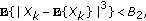


for  where
where  and
and  are positive values.
To apply the LF-CLT in Section 4.3, first we prove that the sufficient conditions are satisfied under  (in the following we assume
  for simplicity). Note that we can write
  as
as

where  for
for  and
and  for
for  . Under
  , it can be seen from (13) that
  is a Binary random variable with mean
  and variance
  . Similarly,
  is a Binary random variable with mean
  and the variance
  . Then assuming perfect communication channels (such that
  ) we have

where last inequality results because  . Note that from (11), if the local false alarm probability
  is set such that
  ,
,  is positive and finite for any
  . Let
. Let  and
and  . Then we have
  and
and  for
for  ,
,  . Similarly, we can show that we can find two positive values
  and
and  such that
  and
and  for
for  ,
,  . Following a similar procedure, it can be shown that the two regularity conditions are satisfied under
  as well.
Rights and permissions
Open Access This article is distributed under the terms of the Creative Commons Attribution 2.0 International License (https://creativecommons.org/licenses/by/2.0), which permits unrestricted use, distribution, and reproduction in any medium, provided the original work is properly cited.
About this article
Cite this article
Wimalajeewa, T., Jayaweera, S.K. Distributed Detection of Randomly Located Targets in Mobility-Assisted Sensor Networks with Node Mobility Management. EURASIP J. Adv. Signal Process. 2010, 695026 (2010). https://doi.org/10.1155/2010/695026
Received:
Revised:
Accepted:
Published:
DOI: https://doi.org/10.1155/2010/695026