
Abstract
We present a level set-based method for object segmentation in polarimetric synthetic aperture radar (PolSAR) images. In our method, a modified energy functional via active contour model is proposed based on complex Gaussian/Wishart distribution model for both single-look and multilook PolSAR images. The modified functional has two interesting properties: (1) the curve evolution does not enter into local minimum; (2) the level set function has a unique stationary convergence state. With these properties, the desired object can be segmented more accurately. Besides, the modified functional allows us to set an effective automatic termination criterion and makes the algorithm more practical. The experimental results on synthetic and real PolSAR images demonstrate the effectiveness of our method.
1. Introduction
Polarimetric synthetic aperture radar (PolSAR) is a well-established multidimensional SAR technique based on acquiring earth's surface information by means of using a pair of orthogonal polarizations for the transmitted and received electromagnetic fields [1, 2]. The object segmentation of PolSAR image plays an important role of PolSAR image understanding and analysis. In this paper, we focus on the problem of PolSAR image object segmentation. In literature, active contour model was well known to automatically recover the shape of objects from various types of images and provide a good detection of object boundaries in PolSAR images [3]. In [4–6], several PolSAR image object segmentation methods based on the classical snake model [5] were proposed. But the classical snake model presents one limitation that topological changes which occur during the curve evolution are difficult. Because the snake model discretizes a curve using a set of points, this representation is hard to describe the curve topological changes.
In [7], a single-look PolSAR image segmentation algorithm based on level set and complex Gaussian distribution is proposed. In [8], a PolSAR image segmentation method is developed by embedding complex Wishart distribution into level set and active contour model. In [9, 10], these level set-based methods in [7, 8] are improved by a new multiphase method which embeds a simple partition constraint directly in curve evolution for PolSAR image segmentation. The level set-based methods can overcome topological change difficulties because level set has the significant advantage of allowing, in natural and numerically stable manner, variations in the topology of active contour [11].
However, the previous level set-based PolSAR image segmentation methods [7–10] may result in an unexpected state when they are used for object segmentation. That is because the corresponding energy functional which derives from Chan-Vese model [12] may have a local minimum. This limitation makes these algorithms may fail to detect the inside objects or the objects far from the contours. Moreover, it is difficult to set an automatic termination criterion to cease the computation automatically for these methods [7–10], since the value of level set function will not converge to a stationary state.
In [13], a level set-based energy functional, which is a modified version of the Chan-Vese model, has been proposed for bimodal segmentation of optical image. This functional is designed for the images which are not noisy or the images of which the noise is not too high. In [14], we proposed a level set-based energy functional which is a modified functional in [13]. This functional is proposed for segmentation of SAR image which contains high level of speckle noise [15]. The proposed functional in [14] is designed to overcome the influence of speckle noise in one-dimensional (1D) data for SAR image. The above two level set-based energy functional [13, 14] can get a stationary global minimum.
As illustrated in [16], the 1D speckle noise model cannot be extended to multidimensional SAR data directly though SAR polarimetry represents an extension to multidimensional data by the use of polarization wave diversity. PolSAR image segmentation is significantly difficult due to the complexity of the data and the occurrence of multiplicative speckle noise [10].
In this paper, following on from our initial effort in [14], we develop a level set-based bimodal segmentation method for PolSAR image object segmentation using complex Gaussian/Wishart observation models. These models are demonstrated to be effective for PolSAR image segmentation in [5, 7–10]. Besides, we improve the mathematical proof of the stationary property compared to our previous work [14]. At last, we discuss the robustness of our method and the effectiveness of the termination criterion in the experiment.
The rest of the paper is organized as follows. In Section 2, we present the statistic observation models. In Section 3, a new energy functional for PolSAR image object segmentation is proposed. In Section 4, we prove that the functional can arrive at a stationary global minimum. In Section 5, an effective termination criterion for the proposed segmentation method is presented. In Section 6, we deduce a numerical approximation of the proposed method. In Section 7 we show the experimental results of our method on both synthetic and real PolSAR images. The conclusions are given in Section 8.
2. PolSAR Image Speckle Observation Model Description
We use different statistical observation models for single-look and multilook PolSAR image case. Let  be the domain of a PolSAR image and
  the pixel of image.
As [16, 17], a PolSAR sensor measures the  complex scattering matrix
  , for each resolution cell, which relates the components of the scattered electromagnetic field with the illuminating field, for a particular polarization basis. For the liner polarization basis case,

where h and v represent the horizontal and vertical linear polarizations, respectively.  is the scattering coefficient relating the illuminating field with q-polarization and the received field in p-polarization.
  can be decomposed in an orthogonal matrix basis, yielding to the target vector's concept [18]. For the lexicographc decomposition basis, the target vector
  is,
is,

where  indicates transpose. For the backscattering direction, due to the reciprocity theorem under the BSA convention [19], that is,
  ,
,  can be simplified as

In the case of single-look PolSAR images, each pixel x of the image in a homogeneous region  consists of a corresponding vector
  as (3).
As [16, 20, 21], based on the coherent nature of SAR, under the Gaussian scatterer assumption,  can be modeled by a multivariate, complex, zero-mean, Gaussian probability density function (pdf):

where  indicates the complex conjugate transpose and
  denotes the determinant of
  . This pdf is determined by the
  complex, Hermitian, covariance matrix
  , as
, as

where  represents the ensemble average, and * is the complex conjugate of a complex quantity.
To estimate the  in a homogeneous region
  of single-look PolSAR images for the proposed segmentation algorithm in the next section, we use the following maximum likelihood method as [9, 10]:

In the case of multilook PolSAR images,  is estimated substituting the ensemble average by spatial averaging [16, 17]:

where  represents the number of looks, and
  is the covariance matrix of a particular pixel defined as
  .
.
As [22–24], each pixel x of the multilook PolSAR image in a homogeneous region  can be represented by a Hermitian matrix
  as (7).
  follows the complex Wishart pdf:

where  is the matrix trace, and
  is as follows for PolSAR system:

To estimate  in a multilook PolSAR image homogeneous region
  , we use the following maximum likelihood estimation as [8–10]:

3. New Energy Functional for PolSAR Image Object Segmentation
As the descriptions of the PolSAR image speckle models in Section 2, we could make the following assumptions. The PolSAR image consists, at each pixel  , of a matrix
  . When the PolSAR image is single-look,
  is a complex vector as
  and follows a complex Gaussian distribution as (4). When the PolSAR image is multilook,
  is a complex matrix as
  and follows a complex Wishart distribution as (8).
As in [10], let  be the assumed distribution of
  in the region
  . The object segmentation is a partition
  of the image domain.
  is abbreviated to
  below. Segmentation into two classes by Bayesian estimation consists in determining a partition
  of maximum a posteriori probability as follows:

Assuming that  is independent of
  for
for  , and taking the negative of the logarithm in (11), this Bayesian estimation is converted to the following energy function minimization problem:

where energy function  is defined by,

Equation (13) indicates that the minimization of energy function (13) can obtain the correct object segmentation of  . In other words, this turns the problem of object segmentation into a problem of energy function minimization.
In order to solve this function minimization problem by curve evolution and level set, the energy functional based on level set function  in [10] is proposed as follows:

where  is regularization parameter,
  is the level set function, and
  is the 1D Heaviside function, with
  if
if  or
or  if
if  .
.  and
and  are defined by
  and
and  , respectively. The first term is the prior term which is the classic boundary length term [25] for smooth segmentation boundaries. The second and third terms are the likelihood terms which are specified by the observation model.
As [10], the minimization of level set-based energy functional (14) via curve evolution is equivalent to the minimization of (13). And then this turns the problem of object segmentation into the problem of energy functional minimization. That is to say, the contours of the objects can be obtained by the minimization of energy functional (14) concerning level set function  .
.
However, as pointed out in [13], the segmentation method in [10] based on the minimization of the functional (14) has two limitations.
Firstly, the minimizer, which is obtained by the minimization of energy functional (14), may become a local minimizer during curve evolution. Because the likelihood terms of functional (14) are a modified edition of Chan-Vese model [12], this model may sometimes enter into a local minimum, as indicated in [12, 13]. When the minimization of energy functional (14) enters into a local minimizer, the segmentation method by [10] based on (14) may fail to detect the inside region or the objects that are far from the initial zero level set. This situation is also shown in our experiments.
Secondly, when we minimize (14) by curve evolution with respect to  for object segmentation, it is difficult to set an appropriate automatic terminate criterion based on the value of the level set function. This is because the value of the level set function cannot converge to a stationary state by the minimization of the energy functional (14) via curve evolution. In practical application, this limitation makes it hard to decide whether the desired object segmentation has been obtained and then stop the curve evolution automatically.
In order to overcome these two limitations, we modify the likelihood terms of (14) and present the following energy functional for PolSAR image object segmentation:

where  is an arbitrary small positive value, and the other parameters are the same to the functional (14).
As shown in [13], the minimization of energy functional (15) with respect to  by curve evolution is also equivalent to the minimization of energy function (6). In other words, the minimization of the functional (15) will result in a level set function whose zero level set can be the contours that separate the objects from the background.
In order to avoid the occurrence of small, isolated regions in the final segmentation, we take the same prior term as in [10, 25]. The likelihood terms, which are the second and third terms of (15), are specified by observation models. These observation models have been described in Section 2.
The minimization of energy functional (15) by curve evolution can obtain a stationary global minimum. That is to say, the corresponding final contours will detect all the objects in the PolSAR image. Moreover, the modified likelihood terms with shift Heaviside function can confine the range of  , so that the solution always becomes stationary. Due to the above improvements, the objects in the PolSAR image can be fully segmented and a termination criterion can be imposed on the algorithm due to the stationary solution. We present a termination criterion in Section 5.
We prove that the minimization of (15) with respect to  can arrive at a stationary global minimum in Section 4.
4. Proof of the Stationary Global Minimum
We have made two modifications in (14) to obtain (15), multiplying  and using shifted Heaviside functions in the second and third terms of (15). By multiplying
  , the energy functional (15) can get a global minimum. By using shifted Heaviside functions, the values of the level set function will converge to a stationary state. These two properties will be proved as follows.
Firstly, we introduce that multiplying  leads to the global minimum as follows. In (14), the likelihood terms, which are the second and third terms of (14), change only if the sign of
  changes during the curve evolution. However, by multiplying
  in the energy functional (15), the likelihood terms, which are the second and third terms of (15), can reflect the value change of
  , even in the absence of a sign change of
  . As illustrated in [13, 14], this modification of the functional can overcome the local minimum limitation of the Chan-Vese model and guarantee that a global minimum can be obtained with the energy functional (15).
Secondly, we prove that the shifted Heaviside functions can guarantee that the level set function will enter into a stationary state when the energy functional achieves the global minimum as follows.
As indicated in [13, 14], the prior term in (15) does not influence the stationary of the energy functional. Therefore, we do not consider the prior term in the following proof for simplicity. We denote by  the integrand of the energy functional (15):

where the values of  and
and  only depend on the zero level set. The values of
  and
and  are controlled by all the level sets.
From (16), we can deduce that, during the curve evolution, every  with magnitude value
  experiences a change such that
  decreases until
  . This fact can be concluded as Lemma 1.
Lemma 1.
If  is a minimizer for energy functional (16), then
  whenever
  .
.
We put the proof of Lemma 1 in the appendix. By Lemma 1, the magnitude value of  will converge to the interval
  at all points when the level set function achieves the convergence state. Now we only need to consider the case
  . In this case,
  . Hence
  is simplified as
  , where

Because  , we can easily find that if
  , the minimizer of
  can be obtained when
  ; if
; if  , the minimizer can be obtained when
  ; if
; if  , the image may be a homogenous region and there is no object to be obtained. Observing this fact and based on Lemma 1, we have the following theorem.
Theorem 1.
Assume that  is a continuous function. If
  is the minimizer for the energy functional
  in (15), then
  , whenever
  . Here

As indicated in [13] that an image can be approximated by a continuous function, for example, by convolving it with a Gaussian kernel. Theorem 1 will hold in this case. The proof of Theorem 1 based on Lemma 1 has been presented in [13]. Theorem 1 can guarantee that  will enter into a stationary state when
  is the minimizer of the functional (15). The effect of Theorem 1 is also shown in the experiments for PolSAR image object segmentation.
5. Imposition of a Termination Criterion
An effective automatic termination criterion is important for a level set-based PolSAR image object segmentation method when the PolSAR image processing system which employs this segmentation method needs to automatically determine whether the desired objects have been obtained.
There are several existing termination criteria for level set-based PolSAR image segmentation as follows. Firstly, a termination criterion bases on the comparison between the  values of the current and the previous step. Secondly, terminate the curve evolution when the sign of the
  values does not change any more. These criteria are not suitable for they may fail to segment certain regions, for example, inside regions [13, 14].
Generally one could set a predefined number of iterations large enough to detect all the desired regions in the PolSAR image domain. However, this will bring so much unnecessary computation. What is more, the number of iterations is dependent on the initialization of  and the kind of PolSAR image which make it difficult to predefine.
The level set function corresponding to these PolSAR image segmentation methods [7–10] will not be stationary when curve evolution enters into a convergence state; so it is difficult to impose a suitable termination criterion on these methods based on the value of level set function.
Because the  of our method is stationary, which means that the value of
  will be
  or
or  at the converged state, we can easily set a termination criterion for our method based on the measurement of the convergency of
  . We define the "PolSAR step difference energy" (PolSDE) as follows:

We can just measure the PolSDE every time step and terminate the computation automatically when the PolSDE decreases approximate to 0; for example, if  , stop the curve evolution and then obtain the desired segmentation result. The effect and graph of the PolSDE are shown in our experiments.
6. Numerical Approximation
As in [13, 14], we precede the following two steps iteratively to compute minimizer of (15) by curve evolution via the Euler-Lagrange equation. Firstly, keeping  fixed, we compute
  using (6) or (10). Secondly, keeping
  fixed, we solve the following gradient descent flow equation with respect to
  :
:

For the implementation of  , we use the compactly supported regularized version
  which is defined as

We calculate the curvature using

where  ,
,  ,
,  ,
,  ,
, are central difference approximations which is defined in [11] as follows:

We can start with any initial level set function and then obtain the same segmentation result in the steady state because the proposed level set-based energy functional in Section 3 can arrive at the global minimum by curve evolution.
We use the following usual notations as [12, 13]: let  be the time step, and let
  be the grid points. Let
  be an approximation of
  , with
  being the initial
  .
.
As [13], the steps to the implementation with an explicit finite difference scheme are as follows.
-
(1)
Initialize the level set function.
-
(2)
Compute
 and
and  by (6) and (10).
 -
(3)
Compute
 by the following discretization:
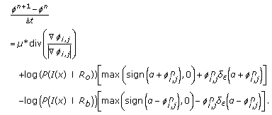 (24)
(24) -
(4)
Calculate the value of PolSDE by (19).
-
(5)
Repeat steps
 ,
,  , and
, and  until PolSDE is less than the threshold,
 and
and  by (6) and (10).
 by the following discretization:
 ,
,  , and
, and  until PolSDE is less than the threshold,
Where  is defined as follows:

7. Experimental Results
In the following, we present several experimental results on synthetic and real PolSAR images to show the object segmentation effect of our method. We display the span image of the PolSAR image in this paper.
We choose the parameters for the experiments as follows. We use  which is defined as [12–14] with
  . According to Theorem 1,
  can be an arbitrary positive value theoretically and we set
  or
or  for the following experiments. It is also shown that different values of
  do not affect the accuracy of segmentation in the experiments. We stop the curve evolution if PolSDE
  . These parameter settings are the same for all the experiments. Only the regularization parameter
  , which has a scaling role [12], is not the same in all experiments. We will give the exact value of
  each time in the following experiments.
In Figures 1 and 2, we compare the segmentation results of our method with the method in [10]. The  function is initialized as a signed distance function. We show the PolSAR images with the corresponding contours.

Comparison of single-look synthetic data object segmentation. (a) Ideal segmentation, size:  . (b)–(e) Segmentation by the method in [10]. (f)–(i) Segmentation using our method with global stationary minimum,
  .
.

Comparison of 4-look synthetic data object segmentation. (a)–(d) Segmentation by the method in [10]. (e)–(h) Segmentation using our method with global stationary minimum,  .
.
The synthetic images of single-look and 4-look are both generated using the ideal segmentation image in Figure 1(a). In Figure 1, we segment single-look PolSAR image. In Figure 2, we segment 4-look PolSAR image. It can be seen that, without a stationary global minimum, the method in [10] fails to detect the inside region and objects that are far from the zero level set, whereas, with our method, all the regions are detected.
Figure 3 shows the evolutions of the  functions with the method in [10] and the proposed method. The value of
  determines the converged state of
  according to Theorem 1. The
  functions are corresponding to the segmentation results in Figures 1 and 2. It can be seen that the magnitude of
  increases with the method in [10] and does not converge. With our method, the value of
  converges to
  . In Figures 3(c) and 3(e), the values of
  converge to 3 or 10, respectively. This proves the effectiveness of Theorem 1.

Evolution of the  function with the method in [10] and our method. (a) Initial for the following experiments. (b) Evolution result with the method in [10] for single-look data. (c) Evolution result with our method for single-look data,
  . (d) Evolution result with the method in [10] for 4-look data. (e) Evolution result with our method for single-look data,
  .
.
In the following experiments we use a very simple initial  function. Half of
  has the value of 1 and half of
  has the value of
  1.
1.
Figure 4 shows the segmentation of the island in a chip of L-band 4-look AIRSAR image in San Francisco Bay. The island in the PolSAR image is the foreground for the object segmentation.

Segmentation result on an AIRSAR image, size:  ,
,  . Left column: PolSAR image and the contours. Right column: corresponding object segmentation results. (a) and (b) Initial; (c) and (d) after 100 iterations; (e) and (f) converged state after 350 iterations.
Figure 5 shows the segmentation of the bridge in a part of L-band 4-look PiSAR image in Niigata. The bridge in the PolSAR image is the foreground for the object segmentation.

Segmentation result on a PiSAR image, size:  ,
,  . Left column: PolSAR image and the contours. Right column: corresponding object segmentation results. (a) and (b) Initial; (c) and (d): after 30 iterations; (e) and (f) converged state after 290 iterations.
We show the effect of the regularization parameter  in Figure 6. Figure 6 shows the experiments on the L-band 4-look AIRSAR image in San Francisco Bay (Figure 4) with
  and
and  . There are many small isolate points in Figure 6(a) with a small weight of regularization term. In Figure 6(b), with a large weight of regularization term, the details of the island contour are lost.

Effect of parameter  on an AIRSAR image, size: 101
  133. (a) Result with
  , and (b) result with
  .
.
Figure 7 shows the segmentation of power transmission towers in a part of L-band 4-look PiSAR image in Niigata. The four power transmission towers in the PolSAR image are the foreground for the object segmentation. In order to evaluate the robustness of the method with respect to different initial conditions, we test the three different initializations represented in Figures 7(a), 7(b), and 7(c). We obtain the same segmentation result as Figure 7(d). All the three different initial level set functions converge to the same object segmentation result. This demonstrates the robustness of our method to different initializations.

Segmentation result on a PiSAR image with different initialization size:  . (a)–(c) Three different initializations. (d) Segmentation result.
We also plot the PolSDE versus iterations in Figure 8, which are corresponding to the three different initializations in Figures 7(a), 7(b), and 7(c). It can be seen from Figure 8 that the values of PolSDE all drop to zero after different numbers of iterations. Therefore, we can easily impose a termination criterion on our method to stop the curve evolution automatically. Furthermore, since our method has a global minimum, it can be seen that an initialization close to the true objects (Figure 7(c)) results in a faster object segmentation process.

PolSDE versus iterations for different initializations.
We show the role of the parameter  in Figure 9. Figure 9 shows the experiments on the 4-look synthetic PolSAR image (Figure 2(a)) with
  and
and  , respectively. According to Theorem 1, the value of
  determines the value to which
  converges. Thus, if we set
  , every
  converges either to 3 or to −3, and if we set
  , they converge to 10 or −10. The results of Figures 9(e) and 9(f) verify Theorem 1. The object segmentation results with different values of
  are the same. That is,
  has the same sign regardless of the value of
  while the magnitude of
  is different.

Effect of parameter  . Left column: the evolution of the
  function with
  . Right column: the evolution of the
  function with
  . (a) Initial, (c) 30 iterations, (d) final result. (b) Initial, (d) 36 iterations, (e) final result.
In Figure 10, we present the object segmentation results by the single channel-based algorithm in [14]. As a contrast experiment, we use the hh and hv channels of PiSAR image in Figure 7. We adopt the same initialization of level set function and the same regularization parameter  . It can be seen from the segmentation results that the power transmission towers cannot be extracted correctly from the single channel of the PolSAR image. However, our algorithm is designed for multidimension SAR data and the corresponding energy functional is derived from the complex Wishart distribution which can characterize the multidimensional SAR data effectively [17]. Thus, our algorithm can extract the information of objects in PolSAR image more accurately than the method in [14] from single channel.

Segmentation results on a single channel of the PiSAR image by the method in [14]. (a) hh channel after 1380 iterations, and (b) hv channel after 2100 iterations.
The proposed algorithm is designed to extract desired objects in PolSAR images, by relying on an active contour model and level set. The resulting contours could be used for high-level PolSAR image analysis, for instance, object recognition. The experiments show that the proposed method outperforms previous level set-based approaches for PolSAR image object extraction in two senses: firstly, it can provide more accurate object extraction results; secondly, an automatic termination criterion can be easily set for the algorithm, which is useful for practical application.
There is a limitation that the accuracy of the proposed algorithm would decrease when the scenes of background are very complicated. The reason lies in the description limitation of the observation model (complex Gaussian/Wishart distribution) adopted by our level set-based method. In complicated scenes, there are several regions of which the scattering mechanisms are similar to that of the desired objects. In this case, the adopted unimodal observation models are not accurate enough to model the background and the foreground, for instance, complicated urban area. Thus, the output of our algorithm may mistake the undesired objects for the desired one because of the inaccurate adopted observation distribution.
One way to overcome this limitation is to use more accurate observation models for such scenes of PolSAR image, for example, the mixture models proposed by [26]. An alternative solution is to introduce some known high-level cues, such as the context information, as a prior to the proposed algorithm.
8. Conclusion
We present a new level set-based bimodal method to segment the objects in PolSAR images. The method has an advantage that it can get a stationary global minimum. This means that the curve evolution will never converge to a local minimum and the value of  in the converged state is predictable. Thereby, the proposed method can detect the desired objects in the PolSAR images well. Moreover, we can set a reasonable termination criterion based on the values of level set function to cease the computation automatically, and this property has practical value in PolSAR image processing.
A major limitation of our algorithm is that for the very complex scenes, the object segmentation accuracy may decrease. The fundamental cause lies in that our method adopts a simple unimodal complex observation model which may be not accurate enough to model some complicated scenes. In view of this point, our plan is to extend the proposed algorithm by using more suitable observation models including mixture model which can describe the complicated scene of PolSAR image more accurately. Also, another plan is to combine other known high-level context information with the proposed algorithm to get a more accurate object segmentation result.
References
Ulaby FT, Elachi C: Radar Polarimetry for Geoscience Applications. Artech House, Norwood, Mass, USA; 1990.
Wong Y, Posner EC: A new clustering algorithm applicable to multispectral and polarimetric SAR images. IEEE Transactions on Geoscience and Remote Sensing 1993, 31(3):634-644. 10.1109/36.225530
Chesnaud C, Rélrégier P, Boulet V: Statistical region snake-based segmentation adapted to different physical noise models. IEEE Transactions on Pattern Analysis and Machine Intelligence 1999, 21(11):1145-1157. 10.1109/34.809108
Goudail F, Réfrégier P: Target detection and segmentation in coherent active polarimetric images. Proceedings of the IEEE International Conference on Image Processing (ICIP '01), October 2001 3: 632-635.
Goudail F, Rélrégier P: Contrast definition for optical coherent polarimetric images. IEEE Transactions on Pattern Analysis and Machine Intelligence 2004, 26(7):947-951. 10.1109/TPAMI.2004.22
Gambini J, Mejail ME, Jacobo-Berlles J, Frery AC: Polarimetric SAR region boundary detection using B-spline deformable countours under the GH model. Proceedings of the 18th Brazilian Symposium of Computer Graphic and Image Processing (SIBGRAPI '05), October 2005 2005: 197-204.
Ben Ayed I, Mitiche A, Belhadj Z: Level set curve evolution partitioning of polarimetric images. Proceedings of the International Conference on Image Processing (ICIP '05), September 2005, Genova, Italy 1: 281-284.
Ben Ayed I, Mitiche A, Belhadj Z: Variational unsupervised classification of polarimetric images. Proceedings of the International Geoscience and Remote Sensing Symposium (IGARSS '06), July-August 2006, Denver, Colo, USA 4198-4200.
Ben Ayed I, Mitiche A, Belhadj Z: Variational unsupervised segmentation of multi-look complex polarimetric images using a Wishart observation model. Proceedings of the IEEE International Conference on Image Processing, 2006, Atlanta, Ga, USA 3: 3233-3236.
Ben Ayed I, Mitiche A, Belhadj Z: Polarimetric image segmentation via maximum-likelihood approximation and efficient multiphase level-sets. IEEE Transactions on Pattern Analysis and Machine Intelligence 2006, 28(9):1493-1500.
Osher S, Fedkiw RP: Level Set Method and Dynamic Implicit Surfaces. Springer, New York, NY, USA; 2002.
Chan TF, Vese LA: Active contours without edges. IEEE Transactions on Image Processing 2001, 10(2):266-277. 10.1109/83.902291
Lee S-H, Seo JK: Level set-based bimodal segmentation with stationary global minimum. IEEE Transactions on Image Processing 2006, 15(9):2843-2852.
Shuai Y, Sun H, Xu G: SAR image segmentation based on level set with stationary global minimum. IEEE Geoscience and Remote Sensing Letters 2008, 5(4):644-648.
Lee J-S, Grunes MR, Mango SA: Speckle reduction in multipolarization, multifrequency SAR imagery. IEEE Transactions on Geoscience and Remote Sensing 1991, 29(4):535-544. 10.1109/36.135815
Lopez-Martinez C, Fabregas X: Polarimetric SAR speckle noise model. IEEE Transactions on Geoscience and Remote Sensing 2003, 41(10, part 1):2232-2242. 10.1109/TGRS.2003.815240
López-Martínez C, Fàbregas X, Pottier E: Multidimensional speckle noise model. EURASIP Journal on Applied Signal Processing 2005, 2005(20):3259-3271. 10.1155/ASP.2005.3259
Cloude SR, Pettier E: A review of target decomposition theorems in radar polarimetry. IEEE Transactions on Geoscience and Remote Sensing 1996, 34(2):498-518. 10.1109/36.485127
Ulaby FT, Elachi C: Radar Polarimetry for Geoscience Applications. Artech House, Norwood, Mass, USA; 1990.
López-Martínez C, Pottier E, Cloude SR: Statistical assessment of eigenvector-based target decomposition theorems in radar polarimetry. IEEE Transactions on Geoscience and Remote Sensing 2005, 43(9):2058-2074.
Ferro-Famil L, Pottier E, Lee J-S: Unsupervised classification of multifrequency and fully polarimetric SAR images based on the H/A/Alpha-Wishart classifier. IEEE Transactions on Geoscience and Remote Sensing 2001, 39(11):2332-2342. 10.1109/36.964969
Conradsen K, Nielsen A, Schou J, Skriver H: A test statistic in the complex wishart distribution and its application to change detection in polarimetric SAR data. IEEE Transactions on Geoscience and Remote Sensing 2003, 41(1):4-19. 10.1109/TGRS.2002.808066
Ferro-Famil L, Reigber A, Pottier E, Boerner W-M: Scene characterization using subaperture polarimetric SAR data. IEEE Transactions on Geoscience and Remote Sensing 2003, 41(10, part 1):2264-2276. 10.1109/TGRS.2003.817188
Lee J-S, Grunes MR, Pottier E, Ferro-Famil L: Unsupervised terrain classification preserving polarimetric scattering characteristics. IEEE Transactions on Geoscience and Remote Sensing 2004, 42(4):722-731.
Mumford D, Shah J: Optimal approximation by piecewise smooth functions and associated variational problems. Communications on Pure and Applied Mathematics 1989, 42: 577-685. 10.1002/cpa.3160420503
Jäger M, Reigber A, Hellwich O: Unsupervised classification of polarimetric SAR data using graph cut optimization. Proceedings of the International Geoscience and Remote Sensing Symposium (IGARSS '08), June 2008, Barcelona, Spain 2232-2235.
Acknowledgments
The authors appreciate the supports of the National High Technology Research, Development Program of China under Grant no. 2007AA12Z155, the National Natural Science Foundation of China under Grants nos. 60872131, 40801183, and 60890074, and LIESMARS Special Research Funding. The authors also thank the editors and anonymous reviewers for their valuable comments, which improved this paper significantly.
Author information
Authors and Affiliations
Corresponding author
Appendix
Appendix
Proof of Lemma 1
Suppose that there exist  such that
  and
and  is continuous at
  . Observe that

Because  and
and  are complex Gaussian/Wishart distributions,
  We choose
  such that
  (or
(or  ) for
) for  , which is the disk centered at
  with the radius
  . Now define the infinitesimal variation in
  as follows:

where  is the characteristic function of
  . With this variation in
  the averages do not change:
 So
So  for
for  .
.
Now, consider the case that  . If
. If  and
and , we have

where the equality holds only if  , or
, or  . Note that
  implies
  since (A.2).
Similarly, if  and
and  , we have

Hence, a minimizer  must be
  , whenever
  . This completes the proof.
Rights and permissions
Open Access This article is distributed under the terms of the Creative Commons Attribution 2.0 International License (https://creativecommons.org/licenses/by/2.0), which permits unrestricted use, distribution, and reproduction in any medium, provided the original work is properly cited.
About this article
Cite this article
Shuai, Y., Sun, H. & Yang, W. Polarimetric SAR Image Object Segmentation via Level Set with Stationary Global Minimum. EURASIP J. Adv. Signal Process. 2010, 656908 (2009). https://doi.org/10.1155/2010/656908
Received:
Revised:
Accepted:
Published:
DOI: https://doi.org/10.1155/2010/656908